The fern cavitation catapult: mechanism and design principles

Abstract

Leptosporangiate ferns have evolved an ingenious cavitation catapult to disperse their spores. The mechanism relies almost entirely on the annulus, a row of 12–25 cells, which successively: (i) stores energy by evaporation of the cells’ content, (ii) triggers the catapult by internal cavitation, and (iii) controls the time scales of energy release to ensure efficient spore ejection. The confluence of these three biomechanical functions within the confines of a single structure suggests a level of sophistication that goes beyond most man-made devices where specific structures or parts rarely serve more than one function. Here, we study in detail the three phases of spore ejection in the sporangia of the fern Polypodium aureum. For each of these phases, we have written the governing equations and measured the key parameters. For the opening of the sporangium, we show that the structural design of the annulus is particularly well suited to inducing bending deformations in response to osmotic volume changes. Moreover, the measured parameters for the osmoelastic design lead to a near-optimal speed of spore ejection (approx. 10 m s^–1). Our analysis of the trigger mechanism by cavitation points to a critical cavitation pressure of approximately −100 ± 14 bar, a value that matches the most negative pressures recorded in the xylem of plants. Finally, using high-speed imaging, we elucidated the physics leading to the sharp separation of time scales (30 versus 5000 µs) in the closing dynamics. Our results highlight the importance of the precise tuning of the parameters without which the function of the leptosporangium as a catapult would be severely compromised.

1. Introduction

Plants have evolved a wide variety of mechanisms to achieve motion and have applied them to numerous functions such as dispersal, nutrition, support and defence [1–3]. Among these mechanisms, the cavitation catapult of leptosporangiate ferns stands out on several counts: (i) it is the fastest plant movement on record [3,4], (ii) it is independent of cellular metabolism, and (iii) it is fully reversible. Considering that these favourable features are all encapsulated within a simple structural design, the fern leptosporangium offers exceptional potential for biomimetic applications [5].

Ferns reproduce by means of spores that develop within a spherical sporangium (figure 1). The small size of the spores (less than 50 µm) allows them to be carried by air currents over great distances. However, the same smallness prevents the spores from detaching easily from the mother plant; hence, the requirement for an active ejection mechanism [6]. In the case of the leptosporangium, a row of 12–25 cells known as the annulus is responsible for spore ejection (figure 1b).

Figure 1.

(a) A fern leaf shows multiple sporangial clusters (sori) on its underside. Two close-ups show an individual sorus and the sporangia within it. (b) Scanning electron micrograph of a partially opened sporangium of Polypodium aureum. The annulus and spores are highlighted in blue and yellow, respectively. (Online version in colour.)

The sporangium catapult mechanism is illustrated in figure 2. Upon reaching maturity, the sporangium is exposed to air allowing water to evaporate through the thin outer walls of the annulus cells. The geometry of the cells is such that the decrease in cell volume forces the thick radial walls to rotate towards each other. It is this rotation of radial walls that drives the opening of the sporangium. The force required to bend the annulus walls during opening is balanced by the negative pressure or water tension that develops inside the cells. When the water tension is too large, cavitation occurs, and bubbles are formed within several cells. Without a continuous column of water to sustain the elastic forces in the annulus walls, the elastic energy is quickly released, leading to fast closure and ejection of the spores as in a catapult (figure 2).

Figure 2.

Schematics of the sporangium action as a cavitation catapult. (a) Closed sporangium with its annular cells filled with water. (b) Opening of the sporangium in response to evaporation at the surface of the annulus. (c) Cavitation within the annular cells. The spores are released in approximately 30 µs. (d) The sporangium after closing. Insets: deformation of the annulus cells during the movement. (Online version in colour.)

Although the ejection mechanism has been broadly understood for over 100 years [7], many of the design features of the leptosporangium have remained unrecognized or misinterpreted to this day. Some of the first quantitative studies focused on measuring the cavitation pressure of the annulus cells. Renner [8] and Ursprung [9], using the same experimental approach, predicted very large negative pressure (−200 to −300 bars), but, as we will show, the value they reported overestimates by a factor of two the true value when all physical factors are taken into account. The first theoretical study of the ejection mechanism focused on an estimate of the ejection speed for the spores based on energy conservation [10]. Later, ultrasound methods confirmed the role of cavitation in triggering the fast closure of the annulus [11]. Noblin and co-workers [4] focused on the closing dynamics, which presents two time scales: a fast initial displacement completed in a few tens of μs and a slower relaxation completed over a period of a few ms. These distinct time scales allow the sporangium to ‘brake’ abruptly midway in the closing motion, increasing considerably the ejection efficiency.

A direct comparison with medieval catapults can help us highlight the design requirements for the sporangium. The leptosporangium is closest in its mode of action to the onager catapult (figure 3a). In essence, the leptosporangium and the onager are mechanisms whereby a tension is used to store elastic energy in rotating elements. However, in contrast to the onager, which possesses a rigid arm rotating about a single point, the leptosporangium possesses many flexible cells, each making a small contribution to the total rotation. This leads to our first design question: how do the geometrical and mechanical properties of the annulus cells promote a catapult motion over all other possible modes of deformation?

Figure 3.

The onager catapult according to a 1727 engraving of Polybius. (a) Illustration of the arm action during launch. Rotation of the arm about its point of insertion is the only degree of freedom available with this design. (b) Design requirement 1: tuning of the skein elasticity with the force that can be developed by the human operators. (c) Design requirement 2: trigger mechanism allowing the stored energy to be freed at once. (d) Design requirement 3: arrest of the arm rotation to ensure ejection of the projectile. (Online version in colour.)

The action of the leptosporangium as a catapult is dependent on three other design requirements (figure 3b–d). First, the material properties of the torsion spring must be commensurate with the force or work available to load it. For the onager, this requirement means that the so-called skein (i.e. the elastic bundle used to actuate the catapult arm) must be tuned such that it can be loaded by human operators (figure 3b). For the leptosporangium, the elasticity of the annulus wall must match the strength of water under tension. Second, the catapult must possess a trigger mechanism to free all the elastic energy at once. For the onager, there is no particular challenge, because the energy is stored in the skein, and only one degree of freedom is available. For the leptosporangium, several cells must cavitate simultaneously. Third, the catapult arm must brake abruptly to release the load. The onager, without a crossbar, would accelerate throughout its course and cast its projectile into the ground.

In what follows, we present a detailed study of the three stages of spore ejection (§§3.1–3.3) and use this quantitative information to evaluate how optimal the design of the catapult is (Discussion). The details of the models and the refilling dynamics of the annulus cells are presented in appendices A.1–A.5.

2. Material and methods

2.1. Sample preparation

All our experiments were performed on the sporangium of the fern Polypodium aureum, whose structural characteristics are shared by a broad range of ferns [12], including the geometry of its annulus, which consists of 13 cells. Sporangia were separated from mature sporangial clusters (sori) and stored individually in distilled water. To allow easy handling of the sporangia, their pedicels were exposed temporarily to air, so that they could be glued to a glass capillary and then stored in water.

2.2. Control of external water potentials

To actuate the sporangia, we either exposed them to air or immersed them in solutions of calcium chloride (CaCl₂). The annulus deformation under these conditions is controlled by the effective water potential of the environment. For the natural trigger in air, the external water potential Ψ_e is set by the relative humidity according to the relation with R the gas constant, T the temperature, RH the relative humidity expressed between 0 and 1 and V_w the water partial molar volume (typically at 20°C and 1 atm.).

However, precise control of relative humidity is challenging, because equilibrium values are reached very slowly. To circumvent this difficulty, most experiments were performed in osmotic solutions of CaCl₂. The osmotic solution method not only allowed us precise control over the water potential of the environment, but it also provided better imaging conditions as the refractive indices of the annulus and the surrounding fluid were more closely matched. We used a standard equivalence table to relate the osmotic potential of the CaCl₂ solutions to relative humidity [13]. The range of concentrations used, between 0 and 2 M, corresponds roughly to relative humidities between 100% and 83%.

As shown below, the osmotic solution method yields results that are quantitatively equivalent to those obtained in air for both the opening and closing dynamics. The repeatability of our measurements shows that the osmolytes used in the experiment do not penetrate into the cells; nor do the osmolytes present in the cell seep out of the annulus. The same conclusion was reached by early investigators [7].

2.3. Microscopy and curvature measurements

The opening and closing of the sporangia were visualized with a PCO-Tech video camera connected to a 10× microscope objective through an optical tube. Other experiments were performed using a Pixelink camera recording at standard video rates and a Phantom v. 7.11 high-speed camera connected to an Olympus IX71 or SZX10 microscope. Sporangia were observed laterally in order to measure the deformation of the annulus (figure 4).

Figure 4.

Experimental set-up for studying the opening, closing and refilling dynamics. In some experiments, a beam splitter was used to observe the fast and slow dynamics concomitantly. (Online version in colour.)

We computed the deformation of the annulus using custom-made image analysis routines implemented in Matlab (The MathWorks Inc.). The geometry of the annulus was characterized using the intersection of radial and inner cell walls, yielding a set of N + 1 points, where N is the number of cells in the annulus. We defined the annulus curvature as the total amount of turning of the annulus divided by its length: (figure 5). For the closed sporangium, immersed into water, the curvature is positive with an initial value As the sporangium opens, its curvature declines and can ultimately reach negative values when the annulus begins to arc back on itself, as shown in figure 2c.

Figure 5.

Sketch of the annulus showing the principal geometrical parameters. The values obtained by direct measurements are shown in the table in the inset. (Online version in colour.)

3. Results

3.1. Loading phase

To study the loading of the sporangial catapult, we measured the temporal evolution of the curvature K in solutions of CaCl₂ covering a broad range of osmotic pressures θ_e (figure 6a). We observed that the curvature decreases rapidly from its initial value K_C, but ultimately converges to an equilibrium curvature, K_∞, as long as θ_e does not exceed the critical value leading to cavitation. As expected for an osmotically actuated catapult, higher osmotic pressures lead to greater annulus deformation (figure 7a) and faster initial rate of opening (figure 7b).

Figure 6.

Opening dynamics of sporangia. (a) Curvature difference versus time for a broad range of osmotic pressures not exceeding the critical value for cavitation. The curves are the best fits using equation (3.1). (b) Curvature difference versus time for different humidity levels (by increasing grey level: 7%, 16%, 30%, 48%, 67% and 82%). Curves are interrupted either by cavitation of the annulus cells before the sporangium has reached its equilibrium curvature or by a strong out-of-plane deformation preventing measurement.

Figure 7.

Characteristics of the opening dynamics. (a) Asymptotic curvature difference versus osmotic pressure of the solutions. The symbols (circles, squares and triangles) represent three experimental series with different sporangia. The black curve is a fit with equation (3.3). (b) Value of the initial slope for the curvature (dK/dt) for aqueous (open squares) and air (filled squares) experiments. The black line is a fit of the linear regime (last four points of the aqueous experiments and first three points of the air experiments). The horizontal line is an average of the measurements made in air at 7.2% and 16% RH.

Similar experiments were performed in air at different relative humidities and showed similar trends (figure 6b). However, for most values of relative humidity (in particular, RH < 75%), the annulus cells cavitate well before the sporangium has reached an equilibrium state. These truncated curves, although closer to what happens under natural conditions, offer only partial information about the osmotic and elastic properties of the annulus.

To be able to rely on osmotic solutions to analyse the mechanics of the sporangium, we checked that the use of an aqueous environment has no adverse effect on the loading dynamics. We first verified that repeated measurements on the same annulus (i.e. triggering and refilling the sporangium multiple times) had no quantitative effect on the measurements (data not shown). We also compared the initial rate of change of the curvature dK/dt for experiments performed in air and osmotic solutions. The experimental points for the two treatments collapse on the same straight line (figure 7b), except for high external osmotic pressures for which the rate of change of the curvature saturates. The good quantitative agreement between the two experimental protocols validates the use of the osmotic solutions to emulate high relative humidities.

The results presented in figures 6 and 7 provide useful quantitative information to evaluate the key parameters controlling the opening of the sporangial catapult. The model for the opening is a simple mass conservation equation whereby the osmotic flux of water across the wall of the annulus cells must be matched by the reduction in cellular volume. The rate of volume change is where the rightmost term is the water potential gradient that consists of the external and internal osmotic pressures (θ_e, θ₀) and the internal hydrostatic pressure (P_i), while L is the wall conductivity and A = wl is the area of the wall through which water flows (see appendices A.1–A.5. for details). Note that the initial osmotic pressure of the cell (θ₀) is modulated by the relative change in cell volume, because the loss of water by the cell leaves behind a cell sap of higher osmotic concentration.

The mass balance can be written directly for the change in curvature using the relation

3.1

where K_C is the equilibrium curvature when the annulus is immersed in pure water (θ_e = 0, the internal osmotic term being equal to θ₀) and K_N is the natural curvature of the annulus when no torque acts on it, hence

3.2

We have also made use of the relation (see appendices A.1–A.5). Two regimes in the curvature evolution (early and late) allow us to estimate some of the parameters in the model. At the beginning of the deformation, i.e. when the rate of change of the curvature is Because θ_e and h are known precisely, the relation above can be used to determine the hydraulic conductivity L. For longer time scales, the curvature reaches its equilibrium value (dK/dt = 0). This condition turns equation (3.1) into a quadratic equation for which the physically realistic root has the form

3.3

where These simple relations and our data for K(t) have allowed us to estimate the physical parameters of this catapult system (table 1).

Table 1.

Value of the key parameters (mean±standard deviation).

parameters	(a) shooting method	(b) asymptotic values	(c) initial slope	(d) closing experiments
h (µm)	34 ± 10	47 ± 20	—	—
L (µm bar–1 s–1)	0.0017 ± 0.0009	—	0.003	—
θ0 (bar)	20 ± 1.4	—	—	20 ± 4.6
B (N m–1)	450 ± 33	380 ± 86	—	—

The physical parameters include the effective height of the annulus cells (h), the bending stiffness of the annulus the hydraulic conductivity of the wall and associated boundary layer (L) and the initial osmotic potential of the cells (θ₀). The last was determined by measuring the difference This is possible from the analysis of the refilling dynamics data (see appendices A.1–A.5). Using equation (3.2), we found 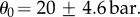To do so, we determined B using iteratively method (a) described below. Three methods were used to determine the other parameters from the opening dynamics (B, h, L):

Method (a): we performed numerical integration of equation (3.1) for each osmotic solution using a shooting method. The obtained dynamics were analysed with a minimization technique to find the parameters (L, B, h) that best fit the experimental data (for osmotic pressures between 43 and 107 bar).

Method (b): at long time scales, the curvature reaches an asymptotic value (K_∞) whose magnitude does not depend on the hydraulic conductivity, because the annulus cells and environment have reached osmotic equilibrium, and, therefore, net water flow has stopped. We used a least-squares method to fit our experimental results for K_∞ to equation (3.3), thus yielding values of h, B for known values of θ₀, K_C and θ_e.

Method (c): according to equation (3.1), the initial rate of change in the annulus curvature is By fitting the initial slope of the curves in figure 6, we obtained the estimate of the ratio for known values of θ_e.

3.2. Triggering phase

We have described how the sporangium stores elastic energy by evaporation of the water contained in the annulus cells leading to high negative pressures (figure 6). The second ejection stage corresponds to the release of this elastic energy by the almost simultaneous cavitation of several cells within the annulus (figure 8a). We experimentally determined the threshold negative pressure required to initiate cavitation. Because cavitation is a probabilistic event, the critical pressure must be determined using a vulnerability curve, i.e. by recording the fraction of sporangia that have cavitated after a fixed period of time (here 850 s) at a given osmotic potential. This curve gives the probability as a function of the external osmotic potential. To express it as a function of pressure, we checked that the cavitation mean time is always equal to or larger than the mean opening time. This means that sporangia are approaching osmotic equilibrium, and taking the asymptotic value of the curvature (K_∞(θ_e)) is a very good approximation to deduce the cavitation pressure using equation (A 9). Our vulnerability curve shows a characteristic ‘S’ shape (figure 8b). For a 50% cavitation probability, we find a critical pressure of bar, where the uncertainty was estimated using extremal values for the parameters B, h and θ₀ (see §3.1 and appendix A.3). This critical pressure value corresponds to an external osmotic pressure of 150 bar or a relative humidity of 89.7%. Therefore, sporangia exposed to levels of relative humidity higher than this level would have low probability of ejecting their spores.

Figure 8.

(a) Cavitation bubbles as they appear soon after triggering of the sporangium. (b) Cavitation probability as a function of the calculated negative pressure in the annulus cells.

3.3. Closing phase

After cavitation, the sporangium swings back to a partially closed configuration, ejecting the spores in the process. We used high-speed imaging to capture the closing phase in sporangia triggered either in osmotic solutions or in air. A quick comparison of the evolution of the annulus curvature during the opening and closing phases highlights the distinct dynamics that underlie these two phases (figure 9a). While the opening phase stretches over several tens of seconds, the closing phase appears instantaneous at those time scales. Using log-linear axes for the closing reveals three different time scales (figure 9b). First, the annulus curvature increases very quickly, followed by damped inertial oscillations with frequency ω₀ and damping time τ (figure 9b, inset). The final motion then consists of two exponential relaxations (τ₁, τ₂ < τ₁).

Figure 9.

(a) Opening and closing dynamics. (b) Fast closing dynamics in log-linear scale. Inset: fast closing phase shows clearly the damped oscillations.

As shown in appendix A.4, the global closing dynamics can be described by the relation

3.4

This relationship is obtained by considering the set of equations describing the quasi-static opening of the annulus, but also taking into account the annulus dynamics as a poroelastic object. The coupling between viscous flows and elasticity (poroelasticity) plays an important role in plant tissues dynamics [3]. As discussed by Skotheim & Mahadevan [2], a beam made of plant tissue can be described with a viscoelastic model composed of a spring (elastic response with characteristic time τ) acting in parallel with a spring and a dashpot (fluid response with characteristic times τ₂ and τ₁). The leptosporangium is a striking example where poroelasticity directly impacts the closing dynamics, allowing efficient discharge of spores. This theme was introduced in a previous publication [4]. Here, we develop a complete model to describe how poroelasticity contributes to the fast closing dynamics (appendix A.4).

We fitted equation (3.4) to our experimental data in order to evaluate the multiple relaxation times and the natural frequency of the annulus. Experiments in air and osmotic solutions led to the same behaviours except for the inertial oscillations that are, as would be expected, slightly more damped in osmotic solutions (see [4]).

We focused in particular on the measurement of ω₀, τ₂ and τ₁. For the inertial oscillation frequency of the annulus (first mode), we measured From our model (see appendix A.4), we have a theoretical value: 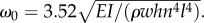Taking the values for w, h, l, and n = 13 determined from the opening and refilling dynamics (table 1), the theory is in good agreement with the measured values, provided a density is used in the calculation. This low value compared with the value for pure water and sporangium material can be explained because of the large volume taken up by the bubbles, and the error in the determination of the parameters.

For the first relaxation time, we measured For the second relaxation time, we measured the ratio Our model gives and where is the water viscosity, k is the permeability of the annulus in m².

By using the measured value of δ and the value determined for EI (using 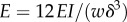), we find E = 6.55 GPa. The theory is in good agreement with the experiments if we take 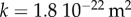for the permeability. This value is lower than common values observed in plants (more in the range ) [14]. For β, the agreement is good in comparison with the error bars.

In addition, our value determined for E depends strongly on the value taken for δ through I. Because the radial cell walls reinforce the inner wall, the effective value for δ may be different, and the Young modulus may be lower than 8 GPa. A higher value of the permeability k would then be logical to explain our experimental value for τ₂.

In conclusion, the value used for EI and then for E deduced from the opening dynamics is in good agreement both for the poroelastic relaxation time and for the inertial oscillations period. Discrepancies can easily be explained knowing that the effective beam thickness and mass have to be used to take into account the complex structural characteristics of the annulus.

4. Discussion

We have shown that the fern leptosporangium uses a water potential gradient to store elastic energy in the annulus. This elastic energy is released abruptly to impart kinetic energy to the spores, thus ejecting them at a velocity of up to 10 m s⁻¹. This subtle sequential transfer of energy is achieved by the annulus, a simple structure consisting of only 13 active cells. The convergence of distinct functions within one structure offers some interesting design challenges which we have attempted to untangle.

4.1. Structural design of the annulus

4.1.1. Global bending/local buckling

The function of the sporangium as a catapult requires that the reduction in cell volume owing to evaporation imparts a bending deformation to the annulus. In other words, the annulus can ‘throw’ the spores only to the extent that it is bent backwards rather than collapsed onto itself. At the cell level, two main deformation modes may occur: (i) a reduction in the cell length l by buckling the base wall locally (up to a complete cell collapse with touching radial walls) and (ii) an annulus bending induced by tilting the radial walls and keeping a constant l. We show here that the annulus geometry has been selected in order to promote the second mode: global bending deformation.

The aforementioned buckling instability, which induces the cell collapse and prohibits large bending deformations, is expected above a critical force exerted on the base wall.

Using the Euler formula, this corresponds to a pressure threshold [15]. The force applied to the radial cell walls is the exerted pressure in the fluid multiplied by the base wall of surface wh. To evaluate this pressure, we took (figure 5) and from our data analysis. We find that the pressure is restricted to The balance between P_L and P_cav imposes a geometrical constraint

Henceforth, the maximum pressure P_L is about 13 times higher than P_cav ( bar) and ensures a very generous safety margin before cells collapse. This means also that, for the tensions reached in the cells, the local buckling deformation is not dominant: the annulus geometry has evolved in order to favour global bending instead of local buckling.

4.1.2. Cell height

Another constraint on the sporangium geometry concerns the height h of the cells. If a sporangium opens completely, its curvature is reversed and it touches itself. The maximum curvature is then given by Thus, large values of h are prohibited in order to reach greater opening curvature and, in the process, store more elastic energy. In his work, King [10] put bounds on the minimal and maximal curvature compared with the cell height, h. Indeed, when the sporangium is closed, it also imposes constraints on h which depend on the number of cells and their length. We can exploit the same kind of approach to deduce expressions for the maximum speed V_m reached by the annulus in two regimes, as a function of h, δ, E and P_cav.

In the first regime (high values of E and δ, and low values of h), the maximum curvature is smaller than K_L and the limiting factor is the cavitation pressure P_cav. In the second regime, the annulus touches itself, so that the curvature cannot increase further. This corresponds to low values of E, δ and high values of h.

4.1.3. Optimal speed

The typical annulus speed is given by the scaling where 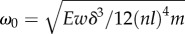and χ is a numerical factor of order 1. For large stiffness, k cannot reach the limit curvature but it is rather limited by the curvature (negative) at which cavitation occurs, In this limit, we predict

4.1

For low stiffness, k_L will be reached quickly upon opening and saturates at The speed will be given by

4.2

The fern movement is limited by the lowest velocity of equations (4.1) and (4.2). When equating both expressions, this leads to the determination of the maximal speed, which we note as V_max. In figure 10, we show the ratio as a function of E and h (assuming δ constant).

Figure 10.

(a) Maximal annulus speed versus cell height h, solid curves: equation (4.1), dashed curves: equation (4.2). (b) Maximal annulus speed versus Young modulus E, solid curves: equation (4.2), dashed curves: equation (4.1).

The main geometrical parameter is then the ratio for which the dependency on V_m shows that an optimal value exists (see figure 10, where is plotted as a function of h). We assumed here that δ was a constant to study the influence of h itself. The optimal value for h is found just above 40 µm, very close to the measured value (36 µm).

4.2. Osmoelastic design

Proper spore ejection requires that cavitation occurs when the annulus has coiled backwards, thus exposing the spores. To achieve the right timing, various parameters must be optimized, such as the bending stiffness of the wall (EI) and the cell's own osmotic potential. We studied earlier the dependence of the maximal annulus speed V_m on E. An excessively supple annulus wall (low EI values) would lead to overcoiling of the annulus before cavitation. Moreover, the elastic energy released and the speed reached by spores would be proportionally small. For an overly stiff annulus, cavitation would occur before the sporangium has sufficiently opened, trapping the spores inside it. Our simple model shows that, considering a limit curvature (when extremal cells are touching) and a cavitation pressure P_cav, the optimal bending stiffness is obtained for This means that cavitation must occur just before the annulus is completely opened. From equations (4.1) and (4.2), the optimal Young modulus E* and velocity are obtained by balancing these two velocities, leading to

4.3

and

4.4

As seen in figure 10, where the speed is plotted as a function of E, our simple model shows the existence of an optimal value for this elastic parameter. As for the height h, the optimal value found here (6.8 GPa) is close to the one determined in §3.3: 6.55 GPa.

4.3. Control over the cavitation pressure

As seen above, the optimal loading of the catapult depends on the cavitation pressure, P_cav. Yet, cavitation is fundamentally a stochastic event. Even under controlled conditions, the point of cavitation can only be predicted in a probabilistic sense (figure 8). How then can a cavitation catapult reliably eject its load? Two aspects of P_cav are important to address this question. First, the value of P_cav must be as high as possible, because it is the negative pressure present in the cells of the annulus that balances the elastic bending stresses in the wall. Meticulous experiments carried out to determine the maximal negative pressure that can be sustained by water yielded values as negative as 220–260 bar [16,17]. Early reports that leptosporangia cavitate at critical pressures ranging from 200 to 300 bar would seem to indicate that leptosporangia have maximized their cavitation pressure [8,9]. In fact, these authors neglected to take into account the osmotic pressure of the cells in their calculation and thus found values exceeding by a factor of two or three our own estimate of 100 ± 14 bar. Our value, however, falls at the upper limit of the range reported for xylem embolism in trees (10–120 bar according to Tyree & Zimmermann [18]). Therefore, leptosporangia have maximized the cavitation pressure in terms of what plants can do.

The second design feature involving P_cav is related to the rate at which the annulus cells approach the critical value. The release of the catapult is characterized by the near instantaneous cavitation of many annulus cells (figure 8). Only such multi-cell cavitation events can guarantee a substantial release of elastic energy and efficient spore ejection. Multi-cell cavitation events probably arise from the initial cavitation of one cell, which sends a shock wave causing neighbouring cells that were nearing the critical pressure to exceed it [19]. For this type of chain reaction to work, many cells must approach the cavitation pressure at the same time. Interestingly, one way to promote such a response is by endowing each cell in the annulus with a non-zero osmotic potential. The internal osmotic potential modifies the way the hydrostatic pressure decreases in cells by providing a second contribution to the cell's water potential which responds to the external water potential or relative humidity. In other words, the cells are approaching the critical cavitation pressure in a geometric progression, allowing several cells to get close to the critical value.

4.4. Poroelastic design

The coupling between porous viscous flows and elasticity (poroelasticity) plays an important role in plant tissue dynamics [3]. Here, we provide an example where it directly impacts the closing dynamics, allowing very efficient discharge of spores. As we have discussed in [4], the main dissipation is internal, and the slow water motion inside the porous media imposes the sudden brake on the annulus, and explains the second characteristic time scale.

Ferns have built an autonomous catapult that is able to control the relaxation of a spring without any structural element. In man-made catapults, such elements were made by crossbeams which were used to arrest the catapult arm in the middle of its throwing motion such that the projectiles were ejected upwardly. Here, the coexistence of two very different time scales (factor of about 200 between them) allows the sporangium to release its spores efficiently by arresting the recoil motion. It imposes a brake after a few tens of microseconds, because time scales from milliseconds up to 1 s are necessary for water to flow inside the porous annulus walls. If the internal poroelastic dissipation was even higher, leading to characteristic time scales of about tens of seconds, then it would impose an additional resistance to the opening dynamics which would lead to premature cavitation. The right order is at least two orders of magnitude between the different time scales ( with and ) and constitutes an optimal poroelastic design between the fast closing and slow opening dynamics.

4.5. Meanings for the reproduction of leptosporangiate ferns

The active dispersal of fern spores described here has reached a level of sophistication that leads to very fast ejection of the spores. This allows first to escape the adhesion of the spores on the sporangium walls, more importantly, it allows the spores to be efficiently carried out of the leaf boundary layer. This layer thickness lies between 1 and 10 mm for low winds for a 30 cm long leaf [20]. Here, owing to air friction, the distance d reached by the spores is of the order of 20 mm This shows that the ejection is sufficient but not excessive, so that spores can be taken by the existing wind away from the plant's influence, and disseminate over large distances. As shown here for ferns, many groups of plants have been very creative in developing such active mechanisms. This mechanism constitutes a great adaptative value to the fern. By tuning various parameters such as annulus cell height or initial osmotic potential, it can adapt to its environment, its humidity level and the average wind values.

Appendix

In this appendix, we derive the key equations describing the phases of the cavitation catapult.

A.1. Evaporation dynamics

The water potential of the external solution is composed of an osmotic term and the pressure outside the cells , which is the atmospheric pressure. In the low concentration regime, the van't Hoff relation [21] links the osmotic term to the external solute concentration by . In our case, the general nonlinear relation [21] is employed, because high concentration has been used (up to 2 M):

A 1

The pressure and the water potential inside the cells are, respectively, P_i and is the concentration of solute inside the cell, with Each cell has a volume V(t) and an initial value The assumption of solute conservation imposes We will assume that inside the cell the linear van't Hoff relation holds, because the corresponding osmotic pressure is about three times lower than outside the cell.

The water flux out of the cell is: J_V in We have [20]. L is the effective permeability. Because water is incompressible, the volume of the cell V obeys the relation A is the area of the membrane. Finally,

A 2

The temporal evolution is, therefore, mediated through the mechanical pressure difference between the intra- and extracellular media, reinforced by osmotic pressure.

A.2. Beam equations

Water leakage induces a change in volume, and, owing to water incompressibility, cell walls deform, and the pressure in the cells decreases. We write the beam equations that describe the mechanics of the annulus, in term of forces and torques. We note that T(s) is the tension on the rod, N(s) is the normal force, and is the mass per unit length of the annulus. We assume the beam to be inextensible and horizontal, and the beam's deformation is measured by Y. We have, for small deformations ,

A 3

and

A 4

The second equation (A 4) is a balance of the internal torque M of the beam. The damping exerted by the exterior fluid (gas or liquid) is related to the Stokes friction. Because the beam is assumed inextensible, we have where measures the angle between the tangent at point s and the horizontal axis. By deriving the previous equation with respect to s, we obtain

A 5

because For the torque balance, we have to consider the torque of shearing forces

A 6

where

• —  is the elastic torque with (we have assumed that the dominant elastic structure is a thin layer of thickness ).

• —  is a poroelastic torque (see later)

• —  is the torque induced by the radial wall of each cell.

An equation for the curvature is derived by differentiating equation (A 5) with respect to s

A 7

where we have used the three torques of (A 4).

A.3. Slow opening dynamics

For the slow opening dynamics, we can neglect the inertial, the friction and the poroelastic terms in equation (A 7), hence we have

A 8

which by integration with respect to s gives the value of the pressure in each cell

A 9

We note K_N, the equilibrium curvature of the annulus after its fast motion. For high deformations, the pressure is linked to the curvature with a nonlinear relation. We keep here the linear assumption. We relate, using the simple trapezoidal cell geometry, the change in volume to the change in curvature: which upon integration becomes For we have we can then write

A 10

Inserting equations (A 10) and (A 9) into equation (A 2), introducing assumed constant, and we find

A 11

In pure water, we have we then find

A.4. Fast closing dynamics

Two simple classical limits exist for this problem: (i) inertia dominates the dissipation, and the beam oscillates around the resting position, at its natural frequency and (ii) the viscous dissipation dominates and leads to an exponential relaxation of the curvature towards its equilibrium value. One of these two behaviours is usually observed in regular elastic beams, depending on the beam properties and the dissipation mechanism, possibly with damped oscillations. Here, we will see that both behaviours are observed sequentially with a two-step motion associated to very different characteristic time scales. Using high-speed imaging, we measure the return to the initial curvature and show that the mechanical annulus behaves in fact as a viscoelastic solid, hence it presents both kinds of motions sequentially: ‘instantaneous’ elasticity (in fact limited by inertia) then viscous relaxation.

Inspired by the calculation for a cylindrical rod from [22], we compute the poroelastic torque for a beam with a rectangular cross section (thickness δ and width l)

A 12

with and . are the Lamé coefficient, is the bulk modulus and is the fluid volume fraction. We define The system can be written in term of coupled differential equations

A 13

and

A 14

This form permits the physics at play to be interpreted. There are an infinite number of flow modes inside the poroelastic media which are responsible of curvature K_n, associated with a critical time scale The parameters measure the characteristic time the liquid flows inside the porous media. Equation (A 7) becomes

A 15

and

A 16

We approximate the spatial dependence to the first deformation mode assuming that it is proportional to where as consequence, we deduce a set of coupled differential equations

A 17

and

A 18

We have derived from the beam equations the dynamics of the fast closing. For a better understanding, this approach can be simply translated in terms of a dashpot/spring mass system made of a viscoelastic medium as presented in figure 11. The dynamics can be described by

A 19

where x measures the position of an object of mass m submitted to various forces induced by springs and dampers

A 20

k_e is the stiffness of the main spring and x is equivalent to the curvature of the annulus. The couples define a pair of springs/dashpots. This is a generalized Maxwell model [23]. A representation of this system is shown in figure 11.

Figure 11.

(a) Equivalent mechanical model for the annulus: a generalized Maxwell model. (b) Using an adiabatic approximation for n > 2 leads to a simplified model.

For n > 2, the characteristic times are short enough to eliminate adiabatically the dynamics of the term because they rapidly tend to the value We then reduce the system into

A 21

A 22

A 23

A 24

We have We further rewrite the system as

A 25

A 26

A 27

where 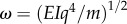is a characteristic beam oscillation frequency, and measures the ratio between the effects of poroelasticity and the elasticity. In the spring/dashpot analogy, the large separation of the characteristic time scales permits the reduction to those shown in figure 11b.

We now present the typical dynamics exhibited by equation (A 25). If the time scales for the dampings are well separated, i.e. the system will first obey equation (A 25), in which K₁ and K₂ can be assumed constant. As a consequence, the curvature K relaxes with oscillations to the value K=K*

A 28

with a frequency with an exponential decay of This is what we have termed the inertial regime, because oscillations are observed in this stage.

Once the curvature K has been relaxed to its equilibrium K*, the relation (A 28) is inserted into equations (A 26) and (A 27), which reduces the previous set of equations to

A 29

and

A 30

As the variable K₁ evolves much more slowly than K₂, can be neglected in equation (A 30), such that K₂ evolves with the characteristic time scale Finally, for asymptotic times, K₂ relaxes to 0; meanwhile is almost constant. Equation (A 29) becomes

A 31

and we deduce that K₁ dynamics is relaxed with a characteristic time Because we only have analysed the linear dynamics, we can sum up the solutions obtained by the scale separation. The curvature then varies as

A 32

The parameters A, B, C are related to the initial conditions and cannot be determined through this model. is the natural pulsation of the beam inertial oscillations (first mode) [15].

The two relaxation times associated with the poroelastic dynamics are and with where is the liquid viscosity, is the permeability and the porosity of the cell wall constituting the annulus.

A.5. Refilling dynamics

In nature, the sporangium keeps on drying after ejecting its spores. Thus, from a physiological or ecological standpoint, the leptosporangium is an irreversible catapult. Nevertheless, if the sporangium is immersed back in water for a few minutes, then the cells refill, the cavitation bubbles disappear and their gases diffuse into the solution. The refilling of the sporangium follows two stages (figure 12). The inward flow of water first causes the cavitation bubbles to reduce in volume until their complete disappearance. Following their removal, water keeps entering the cell until mechanical equilibrium is reached: the catapult has been reset.

Figure 12.

(a) Evolution of the curvature from to during the refilling. The solid curve is the prediction obtained from the model (equations (A 35) and (A 43)). (b) Evolution of the equivalent radius of the bubble. The solid curve shows the prediction obtained from the model (equations (A 35) and (A 43)).

The equilibrium curvature at the end of the reloading process is not the natural curvature, imposed by the elastic structure. A positive pressure is built from to as water continues to enter the cells beyond the atmospheric pressure. This additional positive pressure is an osmotic pressure. The closing motion to the final state is therefore driven by the solutes contained in the cells. As already mentioned, measuring leads to a value for The positive pressures generated allows a quick dissolution of the bubbles.

The bubbles are composed of water vapour and gas which was originally dissolved in the water. As a consequence, the bubble radius dynamics is related to the gas fluxes towards the fluid, and the elastic response of the compressed gas. The presence of the bubble tends to increase the solute concentration and consequently modify the osmotic pressure.

At the early stages of the closure, the bubbles have an ellipsoidal shape which evolves towards a spherical shape (for t < 100 s). We capture this effect by measuring the bubble size in two orthogonal directions. From the side view (i.e. for which the cross section of the cell is l h), the bubble is circular with radius From the front view (i.e. the cross section of the cell is w l), the bubble is ellipsoidal: the semi-major axis is and the semi-minor axis is We define the equivalent radius as where the bubble volume is The experimental measures of K and R are shown in figure 12.

We propose here a model for the refilling dynamics. The cell (of volume ) is occupied with liquid and a bubble considered as a sphere of radius R, hence The variation of the liquid volume in the cell is

A 33

where we have assumed that the fluid is composed of pure water with and A = lw. The volume and geometry of the cell are linked by

A 34

We consequently get

A 35

To close the system, we need to provide an evolution equation for the bubble radius R. The latter is composed of water vapour at constant pressure and a gas assumed to be perfect with partial pressure The Laplace law couples the liquid pressure to the gas pressure

A 36

The parameter r measures the ratio of the number of the dissolved gas molecules to the number of water molecules. The right-hand side is the total pressure inside the bubble. is the surface tension, is the universal gas constant, M is the molecular mass, is the density of the gas and T is the assumed constant temperature.

We approximate the mass of the bubble with which can vary through mass flux from its surface. We assume that the liquid has initially a concentration of the dissolved gas. The mass changes follow the relation [24]

A 37

where is the diffusivity of the gas, and is the dissolved gas concentration for a saturated solution at pressure

A 38

is the Henry constant (for nitrogen ). Because the water is exposed to atmospheric pressure, we have We first neglect the explicit temporal dependence in equation (A 37): during a 1 s experiment, Plugging the relation (A 38) into (A 37) gives

A 39

We also need the following relations obtained by deriving and with respect to time:

A 40

and

A 41

Inserting the second relation into the first one, we obtain

A 42

Using equations (A 39) and (A 42), we finally get the equation for R

A 43

The refilling dynamics is defined through the three variables R, K and which obey the three equations (A 35) (A 36) and (A 43). We have numerically integrated these equations. Their predictions, in comparison with experiments, are quite satisfactory (figure 12).

In the first stage, the curvature increases from whereas the bubble radius R decreases. As the bubble disappears, equation (A 43) reduces to

A 44

which admits as solution

A 45

and is the usual law for the bubble disappearance, as its gas flows into the fluid [24].

In the second stage, the bubble has completely disappeared and the curvature equation becomes

A 46

which may be recast as

A 47

and

A 48

As the elastic response dominates the osmotic forcing, and the relaxation time scale becomes

A 49

This characteristic time is the same as for the opening (see appendix A.3).

Authors' contributions

C.L., M.A., J.D. and X.N. designed the research, C.L., J.W., and X.N. performed the experiments, C.L., M.A., N.R., J.D. and X.N. analysed data, and C.L., M.A., J.D. and X.N. wrote the paper.

Competing interests

We declare we have no competing interests.

Funding

X.N. and J.D. acknowledge financial support from the Material Research Science and Engineering Center at Harvard University, where this project was initiated. Additional support was provided by the CNRS through an ‘Interdisciplinary risk project: EVAPLANT’, the ANR through a young researcher contract ‘CAVISOFT: ANR- 2010-JCJC-0407 01’, and Federation Doeblin (FR 2800 CNRS-Université Nice Sophia-Antipolis). Finally, J.D. acknowledges financial support from Fondecyt under the project: ‘Biophysical Principles Behind Fog Collection in Plants (1130129)’.

References

- 1.Ingold CT. 1939. Spore discharge in land plants. Oxford, UK: The Clarendon Press. [Google Scholar]
- 2.Skotheim JM, Mahadevan L. 2005. Physical limits and design principles for plant and fungal movements. Science 308, 1308–1310. ( 10.1126/science.1107976) [DOI] [PubMed] [Google Scholar]
- 3.Dumais J, Forterre Y. 2012. Vegetable dynamics: the role of water in plant movements. Annu. Rev. Fluid Mech. 44, 453–478. ( 10.1146/annurev-fluid-120710-101200) [DOI] [Google Scholar]
- 4.Noblin X, Rojas NO, Westbrook J, Llorens C, Argentina M, Dumais J. 2012. The fern sporangium: a unique catapult. Science 335, 1322–1322. ( 10.1126/science.1215985) [DOI] [PubMed] [Google Scholar]
- 5.Borno RT, Steinmeyer JD, Maharbiz MM. 2006. Transpiration actuation: the design, fabrication and characterization of biomimetic microactuators driven by the surface tension of water. J. Micromech. Microeng. 16, 2375–2383. ( 10.1088/0960-1317/16/11/018) [DOI] [Google Scholar]
- 6.Martone PT, et al. 2010. Mechanics without muscle: biomechanical inspiration from the plant world. Integr. Comp. Biol. 50, 888–907. ( 10.1093/icb/icq122) [DOI] [PubMed] [Google Scholar]
- 7.Prantl K. 1886. Die Mechanik des Rings am Farnsporangium. Ber. Deutsch. Bot. Gesell. 4, 42–51. [Google Scholar]
- 8.Renner O. 1915. Theoretisches und experimentelles zur Kohäsionstheorie des Wasserbewegung. Jahr Wiss. Bot. 56, 617–666. [Google Scholar]
- 9.Ursprung A. 1915. Über die Kohäsion des Wassers im Farnannulus. Ber. Deutsch. Bot. Gesell. 33, 153–162. [Google Scholar]
- 10.King AL. 1944. The spore discharge mechanism of common ferns. Proc. Natl Acad. Sci. USA 30, 155–161. ( 10.1073/pnas.30.7.155) [DOI] [PMC free article] [PubMed] [Google Scholar]
- 11.Ritman KT, Milburn JA. 1990. The acoustic detection of cavitation in fern sporangia. J. Exp. Bot. 41, 1157–1160. ( 10.1093/jxb/41.9.1157) [DOI] [Google Scholar]
- 12.Haider K. 1954. Zur Morphologie und Physiologie der Sporangien leptosporangiater Farne. Planta 44, 370–411. ( 10.1007/BF01940087) [DOI] [Google Scholar]
- 13.Milburn JA. 1979. Water flow in plants. London, UK: Longman. [Google Scholar]
- 14.Steudle E. 1989. Water flow in plants and its coupling to other processes: an overview. In Methods in enzymology, vol. 174 (eds Fleischer S, Fleischer R), pp. 183–225. London, UK: Academic Press. [Google Scholar]
- 15.Landau LD, Lifshitz EM. 1986. Theory of elasticity, 3rd edn Oxford, UK: Butterworth-Heinemann. [Google Scholar]
- 16.Debenedetti PG. 1997. Metastable liquids: concepts and principles. Princeton, NJ: Princeton University Press. [Google Scholar]
- 17.Caupin F, Herbert ECR. 2006. Cavitation in water: a review. C. R. Phys. 7, 1000–1017. ( 10.1016/j.crhy.2006.10.015) [DOI] [Google Scholar]
- 18.Tyree MT, Zimmermann MH. 2003. Xylem structure and the ascent of sap, 2nd edn Berlin, Germany: Springer. [Google Scholar]
- 19.Noblin, et al. Submitted.
- 20.Nobel PS. 2005. Physicochemical and environmental plant physiology, 3rd edn Burlington, MA: Elsevier Academic Press. [Google Scholar]
- 21.Landau LD, Lifshitz EM. 1996. Theory of elasticity, 3rd revised edn Oxford, UK: Butterworth-Heinemann. [Google Scholar]
- 22.Skotheim JM, Mahadevan L. 2004. Dynamics of poroelastic filaments. Proc. R. Soc. Lond. A 460, 1995–2020. ( 10.1098/rspa.2003.1270) [DOI] [Google Scholar]
- 23.Oswald P. 2009. Rheophysics, the deformation and flow of matter. Cambridge, UK: Cambridge University Press. [Google Scholar]
- 24.Epstein PS, Plesset MS. 1950. On the stability of gas bubbles in liquid-gas solutions. J. Chem. Phys. 18, 1505–1509. ( 10.1063/1.1747520) [DOI] [Google Scholar]