Abstract
The basal ganglia are a collection of subcortical nuclei thought to underlie a wide variety of vertebrate behavior. Although a great deal is known about the functional and physiological properties of the basal ganglia, relatively few models have been formally developed that have been tested against both behavioral and physiological data. Our previous work (Ashby FG, Crossley MJ. J Cogn Neurosci 23: 1549–1566, 2011) showed that a model grounded in the neurobiology of the basal ganglia could account for basic single-neuron recording data, as well as behavioral phenomena such as fast reacquisition that constrain models of conditioning. In this article we show that this same model accounts for a variety of appetitive instrumental conditioning phenomena, including the partial reinforcement extinction (PRE) effect, rapid and slowed reacquisition following extinction, and renewal of previously extinguished instrumental responses by environmental context cues.
Keywords:
appetitive instrumental conditioning is a type of learning in which rewarded behaviors increase in frequency and punished behaviors become less likely. This kind of learning allows us to detect and exploit causal relationships between our actions and rewarding outcomes. Thus the mechanisms underlying appetitive instrumental conditioning play a vital role in our most basic adaptive behaviors.
Early learning theories explained instrumental conditioning with concepts such as drive reduction and habit formation (Hull 943), which led to several influential mathematical models of reinforcement-based learning including Bush and Mosteller's (1951) simple model of instrumental conditioning, Estes's stimulus sampling theory (Estes 1950, 1955), and the well-known Rescorla and Wagner (1972) generalization of Bush and Mostellar's (1951) model. Each of these models share the critical assumption that behavior is derived from stimulus-response (S-R) associations that are learned on a trial-by-trial basis and depend on reinforcement.
These early theories are limited in two major ways. First, they fail to account for behavioral phenomena such as rapid reacquisition, renewal, spontaneous recovery, and other phenomena that suggest that extinction does not erase the original learning. These theories assume that extinction reduces the strength of S-R associations; they have no other mechanism to attenuate responding. The second major limitation is that they lack neurobiological detail. They were developed in a time when the critical neurobiology was only beginning to unfold.
More recently, several mathematical models of instrumental conditioning have been proposed that can account for extinction-based phenomena (Gershman et al. 2010; Redish et al. 2007). While these models assume that instrumental behavior is at least partly driven by learned S-R associations, they also assume a second learning process that allows different S-R associations to be learned in different contexts (this is the key feature that allows them to account for savings in relearning). However, like the classic theories before them, they lack neurobiological detail.
Several neurobiologically detailed computational models of instrumental conditioning have been proposed (Ashby and Crossley 2011; Braver and Cohen 2000; Frank et al. 2001, 2004; Monchi et al. 2000; O'Reilly et al. 1999). However, these models are limited in the scope of behavior that they account for compared with their strictly mathematical counterparts. In some cases, the models incorporate only minimal neurobiological detail (but see Gurney et al. 2015). Thus there is a gap in the space of models that capture a large range of behavioral phenomena, and also contain significant neurobiological detail. We aim to reduce this gap by showing in this article that extensions of our earlier model (Ashby and Crossley 2011) naturally account for many additional key behavioral results from appetitive instrumental conditioning.
Ashby and Crossley (2011) assumed that S-R associations encoding operant responses were learned via cortical-striatal synaptic plasticity and that this plasticity was gated by cholinergic interneurons (TANs). Here, we extend the role of the TANs to context-dependent gating, a role that is supported by recent data suggesting that TANs are important in switching between contexts (Bradfield et al. 2013), and that TANs are sensitive to different contextual features (Apicella 2007; Shimo and Hikosaka 2001; Yamada et al. 2004).
Uncovering the mechanisms of context-dependent learning is essential to the design of efficacious interventions that avoid relapse (Bouton and Swartzentruber 1991). For example, drug addiction is often treated in a rehabilitation clinic, and relapse occurs when the patient returns to the original context of their drug use (Higgins et al. 1995). We selected context-dependent phenomena to model that 1) are directly related to the resistance of a behavior to extinction and its propensity for relapse, 2) represent significant challenges to classic models, and 3) have been previously addressed with a qualitatively distinct approach from the one taken here (Gershman et al. 2010; Redish et al. 2007; Gurney et al. 2015), and thereby provide a common point on which to evaluate competing theoretical views.
MATERIALS AND METHODS
Ashby and Crossley (2011) built a spiking neural network model of the direct pathway though the basal ganglia (Fig. 1), with dopamine (DA)-dependent plasticity at key synapses within the striatum and showed that this model could account for basic instrumental conditioning phenomena. They also showed that the simulated neurons in the model produced spike trains that were consistent with single-unit recordings from striatal medium spiny neurons (MSNs) and TANs (striatal cholinergic interneurons) in a variety of conditioning paradigms. This article reports extensions of this model to additional behavioral phenomena that have been classically interpreted as dependent on context-dependent learning. These phenomena also pose a significant challenge for many existing neurobiologically detailed models and represent a classically significant aspect of appetitive instrumental conditioning. Specifically, we model the partial reinforcement extinction (PRE) effect, the slowed reacquisition data of Woods and Bouton (2007), and the renewal data of Bouton et al. (2011). We also note that spontaneous recovery falls naturally out of our simulations of renewal, although we do not explicitly model it.
Fig. 1.
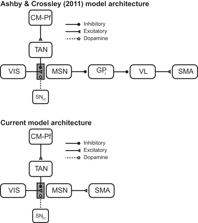
Top: model architecture used by Ashby and Crossley (2011) was based on the direct pathway through the basal ganglia. Bottom: basic model architecture used to model the partial reinforcement extinction (PRE) effect and the data of Woods and Bouton (2007) is a simplified version of Ashby and Crossley (2011). VIS, visual input; MSN, medium spiny neuron; GPi, internal segment of the globus pallidus; VL, ventrolateral nucleus of the thalamus; SMA, supplementary motor area; CM-Pf, centremedian-parafascicular nucleus of the thalamus; TAN, tonically active cholinergic striatal interneuron; SNpc, substantia nigra pars compacta.
Network architecture.
The network architecture used to account for the PRE effect and the slowed reacquisition data of Woods and Bouton (2007) is shown in Fig. 1, bottom. This architecture is a simplified version of Ashby and Crossley (2011; Fig. 1, top) and is characterized by a number of key features. First, instrumental responding is determined by the strength of the synapses between sensory association cortical units and units that represent MSNs in the striatum. The idea is that if one of these synaptic weights is large, then activity in the sensory association cortex will propagate through the direct pathway of the basal ganglia [i.e., through the MSN and internal segment of the globus pallidus (GPi) units] to the ventral lateral (VL) nucleus of the thalamus and finally to the supplementary motor area (SMA) in premotor cortex where a response is generated if the spiking activity exceeds a threshold. Second, the TAN presynaptically inhibits cortical input to the MSN. This means that the MSN can only be excited by sensory cortex when the TAN is paused. Third, the CTX-MSN and centremedian-parafascicular nucleus of the thalamus-TAN (CM-Pf-TAN) synapses are plastic and their strength is modified according to a DA-dependent reinforcement learning rule.
Note that we have greatly simplified the neuroanatomy of the basal ganglia. For example, we do not include GABAergic striatal interneurons, the striosomes (i.e., patch compartments), the ventral striatum, or either the indirect or hyperdirect pathway. Many of these likely play important roles in a variety of relevant behaviors, although few have been explicitly incorporated into formal models of behavior. One prominent exception comes from Frank et al. (2004), who have proposed that the direct pathway learns from positive prediction errors, while the indirect pathway learns from negative prediction errors. Thus the indirect pathway might be expected to play an important role in some of the extinction-based processes we examine here. While interesting, this idea remains speculative, and as we will see, the simpler architecture shown in Fig. 1 is sufficient to account for a wide variety of extinction-based phenomena. The computational cognitive neuroscience simplicity heuristic (Ashby and Helie 2011), which was used to guide the current modeling, recommends not including structure in a model unless it is critical for function or is required by existing data. This heuristic achieves two goals. First, it sets a rigorous criterion on the appropriate level of reductionism; that is, it provides a principled method for deciding what level of detail to include in the model. Second, it guarantees that the resulting model is minimal, in the sense that no simpler model should be able to account for the same data. Therefore, the results described below show that a biologically detailed account of many instrumental conditioning phenomena does not require, for example, the indirect pathway. If the indirect pathway had been included in our model and we achieved equivalently good fits, it would be difficult or impossible to assign appropriate credit for the good fits to the direct vs. indirect pathways.
Simulating the network within trials.
Each trial consisted of 3,000 time steps, and each simulation consisted of 300 acquisition-phase trials and 300 extinction-phase trials. The sensory cortical unit and the CM-Pf unit were modeled as simple square waves. More specifically, the activation of the sensory unit at time t, I(t), was defined as
| (1) |
and the activation of the CM-Pf unit at time t, Pf(t), was defined as
| (2) |
The model of striatal MSN activity was adapted from Izhikevich (2007) and consists of two coupled differential equations. The first equation models fast changes in membrane potential (measured in mV), and the second equation models slow changes in the activation of various intracellular ion concentrations. We additionally assume that the key inputs to the MSN are 1) excitatory inputs from sensory cortex, and 2) presynaptic inhibitory input from the TAN. Thus, the membrane potential MSN unit at time t, denoted S(t), is given by
| (3) |
| (4) |
Here, βS, ES, and σS are constants, w(n) is the strength of the synapse between the sensory cortical unit and the striatal unit on trial n, T(t) is the membrane potential of the TAN at time t, and (t) is white noise. The term [S(t) + 80][S(t) + 25] comes from the quadratic integrate-and-fire model (Ermentrout 1996). Spikes are produced when S(t) = 40 mV by resetting S(t) to S(t) = −55 mV. The last term models noise. When Eq. 3 produces a spike [i.e., when S(t) = 40 mV], uS(t) is reset to uS(t) + 150. All specific numerical values used here are taken from Izhikevich (2007).
The function f[T(t)] in the above equation is a standard method for modeling the time course of the postsynaptic effects caused by presynaptic neurotransmitter release (e.g., Rall 1967). Specifically,
| (5) |
This function has a maximum value of 1.0 and it decays to 0.01 at t = 7.64λ.
The model of TAN firing, which was developed by Ashby and Crossley (2011), successfully accounts for the unusual TAN dynamics in which they fire a quick burst followed by a long pause in response to excitatory input (Kimura et al. 1984; Reynolds et al. 2004). Specifically, we assume that changes in the TAN membrane potential at time t, denoted T(t), are described by
| (6) |
| (7) |
Here, v(n) is the strength of the synapse between the CM-Pf and the TAN on trial n. The constant 950 models spontaneous firing, and the function R(t) = Pf(t) up to the time when CM-Pf activation turns off, and then R(t) decays exponentially back to zero (with rate 0.0018). Spikes are produced by resetting T(t) to T(t) = −55 mV and uT(t) to uT(t) + 150 when T(t) = 40 mV.
Activation in the premotor unit at time t, denoted by M(t), is given by
| (8) |
where ωM, and σM are constants and (t) is white noise. As in other units, spikes are produced after M(t) = 35 by resetting to M(t) = −50.
The model makes a response whenever the output of the premotor unit {f[M(t)]} exceeds a threshold (ϕ). Additionally, the model makes a response on a random 10% of trials independent of the premotor unit output. These random responses are intended to reflect exploratory lever presses (even the most extinguished animal will explore lever presses occasionally). However, we note that these exploratory lever presses are necessary for the model to learn, since before strengthening of the CTX-MSN synapse occurs, motor activity is never above threshold. We also note that this is a feature of every deterministic S-R model. Finally, the CTX-MSN and CM-Pf-TAN synaptic weights (w and v, respectively) are updated immediately after a response is generated or else when the full 3,000 time steps of the trial have elapsed with no response.
Updating the network between trials.
Plastic synapses (CTX-MSN and CM-Pf-TAN) are updated between trials. We follow standard models and assume that synaptic strengthening at these synapses requires three factors: 1) strong presynaptic activation 2) postsynaptic activation that is strong enough to activate NMDA receptors, and 3) DA levels above baseline (Arbuthnott et al. 2000; Calabresi et al. 1996; Kreitzer and Malenka 2008; Reynolds and Wickens 2002; Shen et al. 2008). If any of these factors are missing then the synapse is weakened.
We modeled DA levels according to the reward prediction error (RPE) hypothesis (Glimcher 2011; Schultz et al. 1997; Tobler et al. 2003). The key characteristics of DA firing under this hypothesis are that midbrain DA neurons: 1) fire at a low baseline rate, 2) increase above baseline following unexpected reward, and 3) decrease below baseline following unexpected absence of reward. The magnitude of deviations from baseline depend on the RPE (i.e., how surprising the outcome was), which is defined on trial n as:
| (9) |
where Rn is obtained reward and Pn is predicted reward. We defined Rn as 1 for reinforced responses and 0 otherwise. The predicted reward on trial n + 1 is defined as,
| (10) |
When computed in this way Pn converges exponentially to the expected reward value and then fluctuates around this value until reward contingencies change. We will later see that this property of Pn allows the model to naturally predict the PRE effect and also the slow reacquisition data reported by Woods and Bouton (2007).
We assume that the amount of DA released on trial n is related to the RPE on that trial in a simple manner that is consistent with the DA neuron recording data reported by Bayer and Glimcher (2005):
| (11) |
Note that the baseline DA level (when the RPEn = 0) is 0.2 and that DA levels increase linearly with the RPE. Also note DA increases and decreases are asymmetric. As is evident in the Bayer and Glimcher (2005) data, a negative RPE quickly causes DA levels to fall to zero, whereas there is a considerable range for DA levels to increase in response to positive RPEs. Note, however, that Bayer et al. (2007) showed that the duration of DA pauses also code for negative RPE magnitude. Thus the dynamic range of the DA signal in response to RPEs may be equal for positive and negative RPEs. We performed all simulations and parameter sensitivity analyses reported here with baseline DA set to 0.5 and found that this change made no significant change to any of our results.
Finally, the CTX-MSN synaptic strength, w, and the CM-Pf-TAN synaptic strength, v, are updated on every trial according to:
| (12) |
| (13) |
All integrals in these equations are over the time of stimulus presentation. In practice, we omit the presynaptic activity term ∫I(t)dt because for all applications considered in this article this integral is a constant [because I(t) is a constant] and can be absorbed into the learning rate parameters αw and βw without loss of generality. The function [g(t)]+ = g(t) if g(t) > 0, and otherwise [g(t)]+ = 0. Dbase is the baseline DA level, D(n) is the amount of DA released following feedback on trial n, and αw, βw, θNMDA are all constants.
THE PARTIAL REINFORCEMENT EXTINCTION (PRE) EFFECT
If rewards are delivered after every instrumental response, then training is said to occur under continuous reinforcement. This is contrasted with partial reinforcement, in which reward is withheld following some fraction of responses. An instrumental behavior acquired via partial reinforcement extinguishes more slowly than one acquired under continuous reinforcement. This is called the PRE effect. The PRE effect has been extensively studied and widely observed under a variety of experimental preparations (Jenkins and Stanley 1950; Lewis 1960; Lawrence and Festinger 1962; Robbins 1971; Sutherland and Mackintosh 1971). It has been viewed as a major problem for many learning theories (Mackintosh 1974). Because PRE has been observed under so many different conditions, we chose to not fit the model to any particular data set but instead to show that the PRE effect is a natural a priori prediction of the model.
Methods.
We simulated the model described above in two conditions: Continuous Reinforcement and Partial Reinforcement. The model was trained for 300 trials under continuous reinforcement in the Continuous-Reinforcement condition and for 300 trials under partial reinforcement (i.e., the model received a reward with probability 0.5 after each lever press) in the Partial-Reinforcement condition. After the initial 300 training trials, the model was exposed to 300 additional trials of extinction in each condition in which no reward was delivered for any response.
Results.
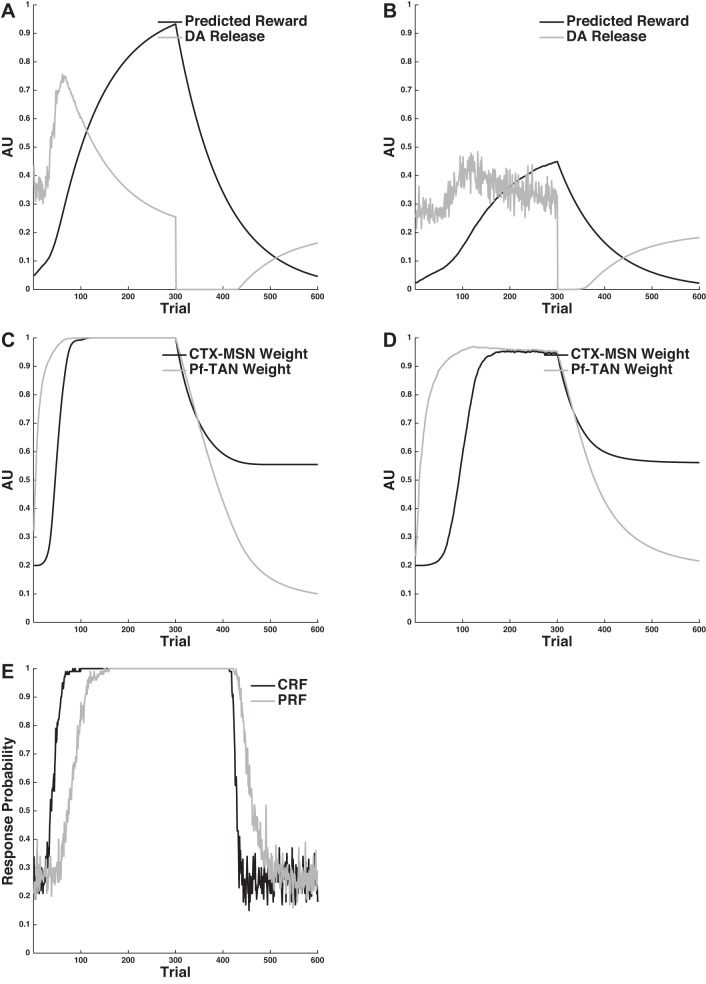
Figure 2 shows the mean results of 50 simulations. Figure 2E shows the model's mean proportion of responses emitted during the extinction phase. Note that responding in both conditions at the beginning of the extinction period is close to 1 (respond on every trial) and that responding decays to near zero (i.e., extinguishes) in both conditions. The key result is that extinction proceeds more quickly in the Continuous-Reinforcement condition than it does in the Partial-Reinforcement condition. Thus the model displays the PRE effect.
Fig. 2.
The PRE effect. A and B: predicted reward and dopamine release in the Continuous-Reinforcement (A) and Partial-Reinforcement (B) conditions. C and D: strength of the CM-Pf-TAN and CTX-MSN synapses in the Continuous-Reinforcement (C) and Partial-Reinforcement (D) conditions. E: response probability in the Continuous-Reinforcement and Partial-Reinforcement conditions. See text for details. AU, arbitrary units.
The PRE effect emerges from the model because of differences in predicted reward estimates under continuous vs. partial reinforcement. To see this, first recall that Pn converges exponentially to the expected reward value, and then fluctuates around this value until reward contingencies change. This is apparent in Fig. 2, A and B, which shows the mean predicted reward and amount of DA released in both conditions across every trial of the simulation. The model's mean predicted reward reaches 1 (perfectly predicted) under continuous reinforcement and only 0.5 under partial reinforcement. This means that reward omission at the onset of extinction will be more surprising (i.e., lead to larger RPEs for more trials) when training occurred under continuous reinforcement than when training occurred under partial reinforcement. This is reflected in the mean DA release (recall that the amount of DA released is proportional to the RPE). Note that DA release is maximally suppressed in both conditions at the onset of extinction but that it recovers to baseline levels in fewer trials when training occurred under partial reinforcement than when training occurred under continuous reinforcement. Since DA remains below baseline for longer in the Continuous-Reinforcement condition, there is more long-term depression (LTD) at the CM-Pf-TAN synapse, which drives responding in the model to zero. Note that the prolonged LTD signals in the Continuous-Reinforcement condition relative to the Partial-Reinforcement condition do not cause much more LTD at the CTX-MSN synapse in the two conditions. This is because the CTX-MSN synapse is protected from decay when the TANs stop pausing (when the CM-Pf-TAN synapse is sufficiently small). This feature of the model is not critical to the PRE effect, but it will be of paramount importance when considering the data of Woods and Bouton (2007) and Bouton et al. (2011).
Discussion.
Many theories of the PRE effect have been proposed since its discovery. One of the most influential accounts was provided by the sequential theory of Capaldi (1967), which assumes that the rate of extinction depends on the similarity between acquisition and extinction reinforcement schedules, with larger differences leading to faster changes in response rate. Applied to the PRE effect, the reasoning is that training under partial reinforcement is more similar to extinction than training under continuous reinforcement because not every response is rewarded. Thus extinction will proceed more quickly when training occurred under continuous reinforcement. Our model can be seen as a biological implementation of this idea, with the similarity between acquisition and extinction captured by the magnitude of the predicted reward term. Large differences between reward predicted on the basis of acquisition experience and reward received during extinction lead to larger RPEs and therefore faster changes in synaptic plasticity.
THE SLOWED REACQUISITION DATA OF WOODS AND BOUTON (2007)
Savings in relearning is a nearly ubiquitous behavioral phenomena observed across a wide range of experimental conditions. In a typical experiment, an animal is trained to press a lever to obtain a food reward. This behavior is then extinguished by removing food delivery, regardless of whether or not the lever was pressed. Finally, reintroducing the food delivery following lever pressing reinstates the behavior. The key finding is that the time to reacquire the lever pressing after extinction is considerably shorter than during original acquisition.
Ashby and Crossley (2011) showed that when an instrumental response is acquired via continuous reinforcement, their model naturally predicts fast reacquisition following a traditional extinction period in which all rewards are withheld. The basic idea is that the sudden omission of expected rewards during extinction causes the TANs to stop pausing (i.e., they remain tonically active). The tonic firing of the TANs inhibits the cortical input to the striatum, which prevents LTD at the cortical-striatal synapse (because there is no longer postsynaptic activity). This preserves the learning during the extinction period. The sudden reintroduction of rewards during the reacquisition phase causes the TANs to start pausing again. Cortical activity is released from tonic TAN inhibition and now excites the striatal MSNs, which causes the behavior to reappear since the critical synaptic strengths were preserved during the extinction period.
Although fast reacquisition following extinction is nearly ubiquitous, there are nevertheless reports of special experimental conditions that can slow, or even abolish, this phenomenon. Woods and Bouton (2007) reported one such example. They used a 2 × 2 design in which one factor was the availability of reward during the extinction phase and the second factor was the availability of reward during the reacquisition phase. During the extinction phase, lever presses were either never rewarded or were rewarded with a very low probability (this probability was titrated down from about once every 32 s at the end of acquisition to about once every 16 min by the end of extinction). They referred to these levels as the Ext and the Prf conditions, respectively. During the reacquisition phase, lever presses were either rewarded about once every 2 min (called the Ext-2 and the Prf-2 groups) or about once every 8 min (called the Ext-8 and the Prf-8 groups). Thus the Woods and Bouton (2007) experiment included the four conditions: Ext-2, Ext-8, Prf-2, and Prf-8. They found that providing sparse rewards during the extinction phase reliably slowed the rate of reacquisition relative to the groups that received no rewards during extinction.
Note that during the acquisition phase, lever presses were rewarded about once every 32 s. This means that lever presses were rewarded considerably less often during the reacquisition phase than during acquisition. In fact, lever presses were rewarded more often at the beginning and middle of the extinction phase in the Prf groups than they were during reacquisition. Nevertheless, there was at least a small increase in the frequency of rewarded lever presses in the reacquisition phase compared with the final components of the extinction phase, and this increase was sufficient to drive a significant increase in lever pressing.
Here, we examine the behavior of the model under the more complex experimental conditions of Woods and Bouton (2007). We find that the model naturally accounts for their main findings; that is, sparsely rewarding lever presses during the extinction phase slows the rate of reacquisition relative to conditions that received no rewarded lever presses during extinction. The behavioral results of Woods and Bouton (2007), and the results of our simulations are displayed in Fig. 3.
Fig. 3.
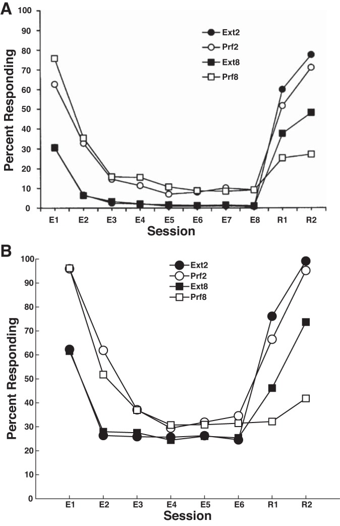
Simulating Woods and Bouton (2007). A: behavioral results from Woods and Bouton (2007). B: simulated results from the model.
Methods.
Each simulation included 300 trials of acquisition, 300 trials of extinction, and 300 trials of reacquisition. The model was provided with reward in a similar way to the animals in Woods and Bouton (2007). During acquisition, the model's responses were rewarded with probability 0.25 for all groups. No responses were rewarded during extinction for the two Ext groups. Responses in the two Prf groups were rewarded with probability 0.14 for the first 10 trials of extinction, 0.12 for the following 10 trials, 0.094 for the following 10, and then 0.047 for the remaining extinction trials. The model's responses during reacquisition were rewarded with probability 0.19 in the Ext-2 and Prf-2 groups, and they were rewarded with probability 0.09 in the Ext-8 and Prf-8 groups.
Figure 3 shows the mean results of 50 simulations presented in a way that mimics the presentation style of Woods and Bouton (2007) as closely as possible. Specifically, we split the 900 trials of the averaged simulation into 18 blocks of 50 trials each. Next, in each block, the dependent measure we report is the percentage of responses emitted during the last block of acquisition. Therefore, for example, a value of 75 means that during that block the model emitted 75% as many responses as during the last acquisition block. Finally, we only display the extinction blocks and the first two reacquisition blocks.
Results.
The results of our simulations are displayed in Fig. 3, bottom. Note that the model correctly captures all major qualitative properties of the Woods and Bouton (2007) data. Specifically, extinction proceeds more slowly and less completely in the Prf groups than it does in the Ext groups, and the Prf groups reacquire more slowly than their Ext counterparts.
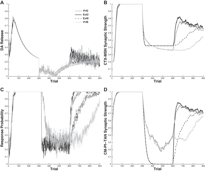
Figure 4 shows the underlying mechanics of the model's behavior. Note that this figure shows the mean results over 50 simulations but is not processed into blocks as in Fig. 3. Figure 4A shows the average DA release; Fig. 4C shows the average proportion of responses emitted; Fig. 4B shows the average synaptic strength of the CTX-MSN synapse; and Fig. 4D shows the average synaptic strength of the CM-Pf-TAN synapse.
Fig. 4.
Simulation of Woods and Bouton (2007). A: average dopamine (DA) release. B: average synaptic strength of the CTX-MSN synapse. C: average proportion responses emitted. D: average synaptic strength of the CM-Pf-TAN synapse.
To see why the model accounts for the Woods and Bouton (2007) data, recall three key features of the model: 1) lever presses are driven through the direct pathway circuit and require a strong CTX-MSN weight; 2) since the TANs presynaptically inhibit the cortical input to the MSN, responses cannot occur unless the TANs pause (even if the CTX-MSN weight is strong); and 3) learning at the CTX-MSN and CM-Pf-TAN synapses is driven by DA, with the amount of long-term potentiation (LTP) or LTD on each trial proportional to the size of DA bursts or dips, respectively. Since DA release is proportional to RPE, DA fluctuations are proportional to how unexpected the outcome is. The sudden omission of expected rewards during extinction causes the TANs to stop pausing (and therefore the model to stop responding) more slowly in the Prf conditions than in the Ext conditions because each occasional rewarded response encountered during extinction in these conditions causes a DA burst and corresponding LTP. This means that CTX-MSN and CM-Pf-TAN synapses experience a mixture of LTP and LTD in the Prf conditions, but only LTD in the Ext conditions. This has the counterintuitive effect of causing more unlearning at CTX-MSN synapses in the Prf conditions than in the Ext conditions. To see why, note that a mixture of LTP and LTD prevents complete unlearning at the CM-Pf-TAN synapse, and therefore, the TANs remain partially paused in the Prf conditions. Thus the CTX-MSN synapse is left vulnerable to unlearning in the Prf conditions relative to the Ext conditions.
Responses during the reacquisition phase in the Ext2 and Prf2 conditions are rewarded considerably more often than in the Ext8 and Prf8 conditions. Since each rewarded response induces LTP at the plastic synapses (i.e., boosts the likelihood of future responses), reacquisition in the Ext2 and Prf2 conditions proceeds more quickly than in the Ext8 and Prf8 conditions. However, the Ext conditions reacquire faster than the corresponding Prf conditions because the CTX-MSN synapse experienced more LTD during extinction in the Prf conditions than in the Ext conditions. Note that with respect to overall response probability during reacquisition, the effect of reward frequency trumps the advantage of Ext relative to Prf extinction; that is, in both the model and in the original data, Prf2 reacquires more quickly than Ext8.
Discussion.
Woods and Bouton (2007) explained their findings by appealing to ideas very similar to Capaldi's explanation of the PRE effect (Capaldi 1967) and Bouton's own trial-signaling view (Bouton 2004). The basic idea of each is that the rate of change in responding is determined by the similarity between training phases. In the case of the PRE effect, the critical similarity was between acquisition and extinction. In the data of Woods and Bouton (2007), the critical similarity is between extinction and reacquisition. In both cases, the idea of similarity includes the schedule of reinforcement. Our account of these data can again be seen as a biological implementation of these ideas. The partial reinforcement used during extinction in the Prf groups prevents the TANs from completely unlearning their pause response. This leaves the instrumental response learned at CTX-MSN synapses subject to more unlearning, and therefore slows reacquisition in the Prf groups relative to the Ext groups.
THE RENEWAL DATA OF BOUTON ET AL. (2011)
Renewal is another well-known paradigm used to demonstrate savings in relearning. The typical renewal paradigm has three phases: acquisition, extinction, and renewal. The acquisition and extinction phases are identical to their fast reacquisition counterparts (i.e., lever presses are rewarded during acquisition but are eliminated during extinction). The renewal phase is essentially another extinction phase in that responses are not rewarded. The key feature of a renewal experiment is that the three phases take place in different environmental contexts. Renewal is said to occur when animals press the lever more in the renewal phase than they did at the end of the extinction phase.
Three forms of renewal are typically examined, ABA, AAB, and ABC. In this nomenclature, each letter corresponds to a distinct environmental context, and the order the letters appear in each triplet represents the three phases of the renewal experiment (i.e., acquisition, extinction, and renewal). For example, in ABA renewal, the acquisition and renewal phases occur in context A and extinction occurs in context B.
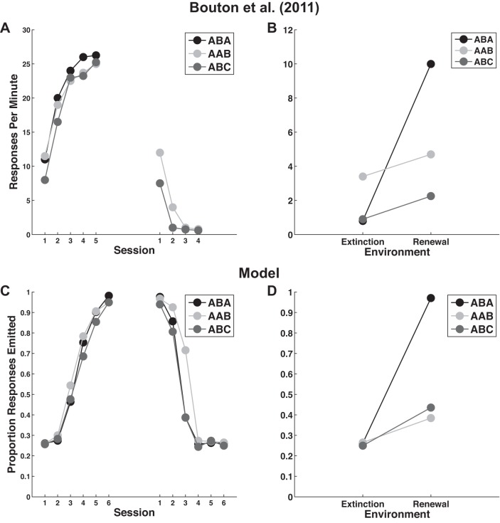
Bouton et al. (2011) performed a set of experiments that demonstrated all three forms of renewal in appetitive instrumental conditioning. The participants in every condition (ABA, AAB, and ABC) received a VI-30-s schedule of reinforcement during the acquisition phase, and reinforcements were completely removed during both the extinction and renewal phases. The results, shown in Fig. 5, A and B, were characterized by several key qualitative attributes: 1) performance during acquisition was equal across groups; 2) the ABA and ABC groups extinguished more quickly than the AAB group; 3) group ABA exhibited the strongest renewal and groups AAB and ABC exhibited considerably less renewal; and 4) although the magnitude of renewal (i.e., the difference in mean responding between the extinction and renewal phases) was similar in groups AAB and ABC, group AAB showed slightly higher responding in both the extinction and renewal phases. The behavioral results of Bouton et al. (2011), as well as the results of our simulations are displayed in Fig. 5.
Fig. 5.
Simulating Bouton et al. (2011). A and B: behavioral results from Bouton et al. (2011) during the acquisition and extinction (A) and renewal (B) phases. C and D: behavioral results obtained from the model during the acquisition and extinction (C) and renewal (D) phases. See text for simulation details.
Methods.
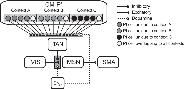
Figure 6 shows the architecture of the model that we used to fit the data of Bouton et al. (2011). Note that this model is identical to the model used to fit the data of Woods and Bouton (2007), except that it included 36 CM-Pf units [as opposed to the single CM-Pf unit used in the Woods and Bouton (2007) application]. Twenty-four of these units were each associated with a single environmental context (8 per context), and the remaining 12 were associated with all three contexts (we refer to these as the “overlap” CM-Pf units). The idea was that CM-Pf units respond uniquely to certain features in the environment but that some units will be tuned to features that are present in all contexts. Every CM-Pf unit projected to the TAN with its own unique synapse, and every CM-Pf-TAN synapse was plastic. The activation during stimulus presentation of CM-Pf unit j in context i, denoted by Pfi,j was given by,
| (14) |
Fig. 6.
Model architecture used to fit Bouton et al. (2011).
The activation of the TAN unit was computed by the following coupled differential equations,
| (15) |
| (16) |
where vi,j(n) is the strength of the synapse between the TAN and the jth CM-Pf unit associated with context i on trial n. The function Ri,j(t) = Pfi,j(t) up to the time when CM-Pf activation turns off, then decays back to zero exponentially with rate 0.0018. All other activation equations were the same as those previously described.
Results.
Figure 5, C and D, shows the mean performance of the model over 100 simulations, presented to mimic the presentation style of the Bouton et al. (2011) results. Specifically, we split the 900 trials of the averaged simulation into 18 blocks of 50 trials each. Finally, in the Fig. 5D, we computed “extinction” performance by taking the average of the last two extinction blocks and “renewal” performance by taking the average of the first two renewal blocks. Note that the model captures the major qualitative results of Bouton et al. (2011). In particular: 1) acquisition performance in the model is equal across all groups; 2) the AAB and ABC groups extinguished more quickly than the ABA group; and 3) group ABA exhibited the strongest renewal effect while groups AAB and ABC exhibited considerably smaller renewal effects.
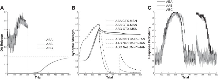
Figure 7 shows the average DA release, CTX-MSN synaptic weight, net CM-Pf-TAN synaptic weight, and response probability over all simulations. Note that the net CM-Pf-TAN synaptic weight is the average weight of all active synapses. Thus, when in context A, the net CM-Pf-TAN synaptic weight is the average of all CM-Pf-TAN weights active in context A (including the overlap units). Note that all conditions are identical until the onset of the extinction phase. Next, note that there is essentially no difference in mean DA release (Fig. 7A) between the three conditions during any phase. This means that the learning signals influencing CTX-MSN and CM-Pf-TAN synapses were identical across all three conditions, and so any differences must be due to the changes in context among experimental phases. Figure 7C shows that the AAB condition is slowest to extinguish, and Fig. 7B shows that this is because the CM-Pf-TAN synapses decay most slowly in this condition. This is because the same CM-Pf-TAN synapses are active in both acquisition and extinction for this condition (context A, in AAB). This means that the CM-Pf-TAN synapses that were strengthened during acquisition (those sensitive to context A) must be weakened in order for the TANs to stop pausing and the model to stop responding. In the ABA and ABC conditions, on the other hand, the active CM-Pf-TAN synapses during extinction (context B units) were not active during acquisition and therefore were not strengthened during initial training. Thus the switch from context A to context B in the transition from acquisition to extinction entailed the switch from strong CM-Pf-TAN synapses to weak CM-Pf-TAN synapses. The transition to weak CM-Pf-TAN synapses means that the TANs almost immediately stop pausing. However, this also means that the context A CM-Pf-TAN synapses were not weakened much during extinction (because they were not active in context B). This is the reason why responding is immediately and robustly renewed in the ABA condition when the context is switched back to A. Responding is renewed to a considerably smaller degree in the AAB and ABC conditions because in each of these cases the context was switched to a novel context whose corresponding CM-Pf-TAN synaptic weights were neither significantly strengthened (to respond robustly) nor weakened (to completely suppress responding) during any prior phase.
Fig. 7.
Model mechanics during simulations of the renewal experiments of Bouton et al. (2011) across all 900 trials computed from the mean of 50 simulations. The acquisition phase included trials 1–300, extinction included trials 301–600, and the renewal phase occurred during trials 601–900. A: DA release. B: CTX-MSN (solid lines) and net CM-Pf-TAN (dashed lines) synaptic weights. C: response probability.
Discussion.
As discussed above, renewal implies that extinction did not completely erase the learning that occurred during acquisition. Bouton et al. (2011) postulated two primary mechanisms via which initial learning could be protected. The first is that the context is part of the stimulus, which means that extinction training in a different context (as in ABA and ABC renewal) would be conditioning with a different stimulus and therefore would not interfere with the initial learning. The renewal effect observed in the AAB and ABC paradigms would then presumably be explained by some type of generalization of the instrumental response to novel contexts. The second possibility is that the context “sets the occasion” for the active reinforcement contingencies. The idea here is that there are two learning processes occurring simultaneously. One of these learns about the instrumental response, and the other learns about the context in which the instrumental response is valid.
The model proposed here is consonant with the latter of these hypotheses. The idea is that the instrumental response is learned at CTX-MSN synapses and the context is learned at CM-Pf-TAN synapses. It is noteworthy, however, that it would be fairly straightforward to incorporate contextual cues into the stimulus representation (i.e., absorb the context information into the CTX-MSN pathway). Even so, we chose not to include contextual cues into the stimulus representation because of strong neurobiological evidence that TANs are broadly tuned (i.e., they respond to stimuli from a variety of modalities), whereas MSNs are more narrowly tuned (Caan et al. 1984; Matsumoto et al. 2001). Thus it seems unlikely that the same MSNs will both drive the instrumental behavior and respond to contextual cues. Several other neural network models have been proposed that include similar mechanisms to the occasion-setting view proposed by Bouton and the context-learning account provided by our model. These other models can account for renewal by assuming that extinction is a process of learning that the environmental context has changed (Gershman et al. 2010; Redish et al. 2007). These models assume two separate processes: a situation recognition process that learns to recognize the current environmental context, and a standard reinforcement learning component. The models are not neurobiologically detailed, although Redish et al. (2007) and Gershman et al. (2010) both speculate that the locus of their context-learning module is within prefrontal cortex and/or the hippocampus.
PARAMETER SENSITIVITY ANALYSIS
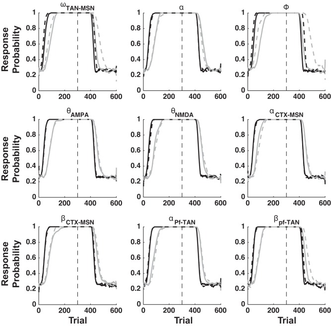
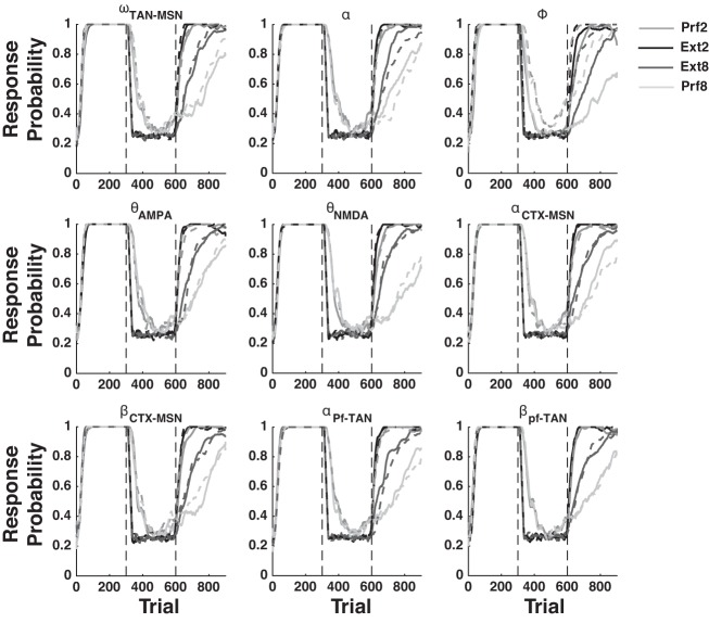
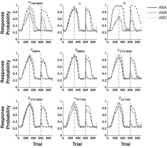
The qualitative output of the model is derived from its fixed architecture, not from its mathematical flexibility. To illustrate this point, we iteratively re-simulated all of our results by first increasing then decreasing the values of nine key parameters by ±5% (see Table 1 for a list and description of these key parameters). Figures 8, 9, and 10 show that the qualitative output of our simulations remain unchanged for nearly every parameter perturbation explored.
Table 1.
Parameters explored for sensitivity analysis
| Parameter Name | Parameter Description |
|---|---|
| ωTAN-MSN | TAN-MSN synaptic strength |
| α | Predicted reward learning rate |
| Φ | Response threshold |
| ΘAMPA | AMPA learning threshold |
| ΘNMDA | NMDA learning threshold |
| αCTX-MSN | ωCTX-MSN LTP rate |
| βCTX-MSN | ωCTX-MSN LTD rate |
| αPf-TAN | νPf-TAN LTP rate |
| βPf-TAN | νPf-TAN LTD rate |
TAN, tonically active cholinergic striatal interneuron; MSN, medium spiny neuron; LTP, long-term potentiation; LTD, long-term depression.
Fig. 8.
Sensitivity analysis for the PRE simulations. See Table 1 for a description of each parameter explored. Solid lines are +5% and dashed lines are −5% perturbations. Black lines are Continuous-Reinforcement, and gray lines are Partial-Reinforcement.
Fig. 9.
Sensitivity analysis for the fits to the data of Woods and Bouton (2007). See Table 1 for a description of each parameter explored. Solid lines are +5% and dashed lines are −5% perturbations.
Fig. 10.
Sensitivity analysis for the fits to the data of Bouton et al. (2011). See Table 1 for a description of each parameter explored. Solid lines are +5% and dashed lines are −5% perturbations.
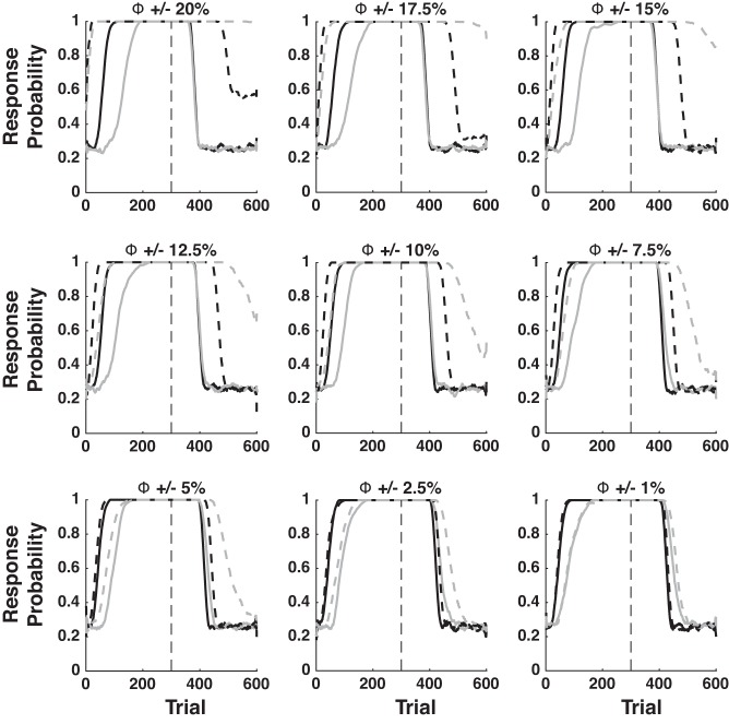
Careful inspection of the PRE sensitivity analysis reveals that the response threshold (Φ) can strongly affect the magnitude of the PRE effect. To understand why, note that changes to response probability trail behind changes in CTX-MSN and CM-PF-TAN weights. This is clearly seen in Fig. 2C, in which CTX-MSN and CM-PF-TAN weights begin to change immediately, but response probability lags behind by ∼100 trials. This is because the CTX-MSN weight is strong enough to drive network activity over the response threshold. The lower the response threshold, the longer it will take for CM-Pf-TAN inhibition to grow strong enough to shut down responding. To examine this effect more thoroughly, we performed an additional sensitivity analysis of the PRE effect, examining changes in Φ at ±20, ±17.5, ±15, ±12.5, ±10%, ±7.5, ±5, ±2.5, and ±1%. These results are shown in Fig. 11. Note that decreases of more than 10% abolish, but do not reverse the PRE effect. Even so, for all other values the effect remains. Thus, even though the quantitative predictions of the model are sensitive to the numerical value of the response threshold (Φ), the model nevertheless robustly predicts the PRE effect.
Fig. 11.
PRE response threshold sensitivity analysis. Solid lines are +% and dashed lines are −% perturbations. As in Fig. 2, black lines denote Continuous-Reinforcement, and gray lines denote Partial-Reinforcement.
GENERAL DISCUSSION
This article showed how TANs might protect learning at cortical-striatal synapses in a variety of instrumental conditioning preparations in which a response is extinguished by removing rewards. The idea is that the TANs exert a tonic inhibitory influence over cortical input to striatal MSNs that prevents the execution of striatal-dependent actions. However, the TANs learn to pause in rewarding environments, and this pause releases the cortical input neurons from inhibition, thereby facilitating the learning and expression of striatal-dependent behaviors. When rewards are no longer available (as in a typical extinction procedure), the TANs cease to pause, which protects striatal learning from decay. Ashby and Crossley (2011) showed that the resulting model was consistent with a variety of single-cell recording data and that it also predicted some classic behavioral phenomena, including fast reacquisition following extinction. This article shows that this model naturally accounts for a broad array of context-dependent appetitive instrumental conditioning phenomena.
Our model is in essence an S-R model (the CTX-MSN component) imbued with a gating mechanism (the CM-Pf-TAN component) that can permit or prevent the expression of learned S-R associations and in so doing permit or prevent changes to the strength of this association. The CTX-MSN aspect of our model can therefore be viewed as a biological implementation of the early S-R models laid out by Hull (1943), Bush and Mosteller (1951), and Rescorla and Wagner (1972). The CM-Pf-TAN component, on the other hand, can be seen as a biological implementation of the context detection modules of later theories proposed by Redish et al. (2007) and Gershman et al. (2010). Importantly, the level of biological detail included in our model, in conjunction with the breadth of behavioral simulations we have presented, is rarely matched in the literature. Thus this work begins to fill a gap in the space of models that capture a large range of behavioral phenomena and also contain significant neurobiological detail.
Relationship to existing biological models.
Gurney et al. (2015) proposed a model of action selection poised in the functional anatomy of the basal ganglia and showed that it naturally accounts for many of the same behavioral phenomena that we account for here and in our earlier work (Ashby and Crossley 2011). Interestingly, the Gurney et al. (2015) model assumes that extinction, in addition to optimal action selection, is driven by learning at CTX-MSN synapses that are on the indirect pathway, an approach fundamentally distinct from our assumption that extinction is driven by learning at CM-Pf-TAN synapses. Although the current evidence cannot resolve this difference, it is also possible that our different approaches are not mutually exclusive. Clearly, more research on these issues is needed.
In actor-critic models, an actor system implements an action selection policy, and a critic system estimates the value of different states and uses these estimates to generate prediction errors, which are then used to update the critic's value estimates and the actor's selection policy. Our model resembles an actor-critic architecture, with CTX-MSN synaptic weights coding the actor, and the DA system coding the critic, and is therefore similar to this earlier work (Houk et al. 1995; Joel et al. 2002; Sutton and Barto 1998). However, our model diverges from classic actor-critic architecture in several important ways. First, the CM-Pf-TAN elements in our model imbue it with biologically plausible context sensitivity not present in classic actor-critic models. Second, the learning rule implemented at CTX-MSN synapses depends on three factors (presyanptic activity, postsynaptic activity, and dopamine), whereas classic actor critic models update their selection policy based only on the prediction error. This latter point is relevant because the TANs are able to protect CTX-MSN weights during extinction because they reduce presynaptic activity, something that would have no effect in classic actor-critic models.
Context-dependent learning by CM-Pf-TAN projections.
There are essentially two current theories of CM-Pf-TAN projections. One assigns this pathway a foundational role in attention and arousal regulation (Kimura et al. 2004). Another suggests a much finer grained role in context recognition and behavioral switching between contexts (Bradfield et al. 2013). This latter view resonates well with our current model of CM-Pf-TAN mediated context-dependent learning. It also resonates well with a body of evidence demonstrating the sensitivity of TANs to contextual features (Apicella 2007; Shimo and Hikosaka 2001; Yamada et al. 2004). Ultimately, however, there remain several ambiguities. The current literature suggesting such a contextual role for the CM-Pf-TAN pathway is sparse and focused on behavioral flexibility (place learning, n-arm maze navigation, etc.), as opposed to the S-R association learning we model here.
Finally, it also seems that the context-sensitive role we attribute to CM-Pf-TAN circuity may be limited to the dorsal striatum. Recent work has shown that TANs in the ventral striatum display somewhat different response characteristics than TANs in the dorsal striatum, which we model here. In fact, recent modeling work of context-dependent fear conditioning suggests a critical role for interactions between ventral-medial PFC (vmPFC), the amygdala, and the hippocampus, and this network is much more closely related to ventral striatal function, than to dorsal striatum (Ji and Maren 2007; Moustafa et al. 2013). Thus one possibility is that both hippocampus-amygdala-vmPFC and CM-Pf-TAN circuits are plausible mechanisms for context-dependent learning, but for different forms of learning.
Multiple systems in instrumental conditioning.
Multiple-systems accounts of instrumental conditioning dissociate “habitual” from “goal-directed” behavior, which are distinguished from each other according to their sensitivity to outcome devaluation and changing response-outcome contingencies (Yin and Knowlton 2006). Specifically, a behavior is considered goal-directed if the rate or likelihood of the behavior is decreased by reductions in the expected value of the outcome, and by reductions in the contingency between the action and the outcome. By contrast, habits are behaviors that have become insensitive to reductions in both outcome value and response-outcome contingency (Dickinson 1985; Yin et al. 2008). Goal-directed behaviors require dorsal-medial striatal networks and habitual behaviors require dorsal-lateral striatal networks (Yin et al. 2004, 2005). Lesion studies show that behavior can switch from goal-directed to habitual and vice versa, suggesting that these two systems learn simultaneously (Balleine and Dickinson 1998; Coutureau and Killcross 2003; Killcross and Coutureau 2003; Yin et al. 2004). The model presented in this article can be seen as a model of the habit system, completely ignoring the goal-directed system. However, it is certainly possible that the goal-directed system plays a role in the behaviors modeled in this article. Our modeling does not suggest otherwise but rather demonstrates that, at least for the behaviors we examined, it is not necessary to appeal to a goal-directed system to account for the observed results.
GRANTS
This research was supported in part by National Institutes of Health Grants P01-NS-044393 and 2R01-MH-063760 and Air Force Office of Scientific Research Grant FA9550-12-1-0355.
DISCLOSURES
No conflicts of interest, financial or otherwise, are declared by the author(s).
AUTHOR CONTRIBUTIONS
Author contributions: M.J.C. and F.G.A. conception and design of research; M.J.C. performed experiments; M.J.C. analyzed data; M.J.C., J.C.H., P.D.B., and F.G.A. interpreted results of experiments; M.J.C. and F.G.A. prepared figures; M.J.C., J.C.H., P.D.B., and F.G.A. drafted manuscript; M.J.C., J.C.H., P.D.B., and F.G.A. edited and revised manuscript; M.J.C., J.C.H., P.D.B., and F.G.A. approved final version of manuscript.
REFERENCES
- Apicella P. Leading tonically active neurons of the striatum from reward detection to context recognition. Trends Neurosci 30: 299–306, 2007. [DOI] [PubMed] [Google Scholar]
- Arbuthnott G, Ingham C, Wickens J. Dopamine and synaptic plasticity in the neostriatum. J Anat 196: 587–596, 2000. [DOI] [PMC free article] [PubMed] [Google Scholar]
- Ashby FG, Crossley MJ. A computational model of how cholinergic interneurons protect striatal-dependent learning. J Cogn Neurosci 23: 1549–1566, 2011. [DOI] [PubMed] [Google Scholar]
- Ashby FG, Helie S. A tutorial on computational cognitive neuroscience: modeling the neurodynamics of cognition. J Math Psychol 55: 273–289, 2011. [DOI] [PMC free article] [PubMed] [Google Scholar]
- Balleine BW, Dickinson A. Goal-directed instrumental action: contingency and incentive learning and their cortical substrates. Neuropharmacology 37: 407–419, 1998. [DOI] [PubMed] [Google Scholar]
- Bayer HM, Glimcher PW. Midbrain dopamine neurons encode a quantitative reward prediction error signal. Neuron 47: 129–141, 2005. [DOI] [PMC free article] [PubMed] [Google Scholar]
- Bayer HM, Lau B, Glimcher PW. Statistics of midbrain dopamine neuron spike trains in the awake primate. J Neurophysiol 98: 1428–1439, 2007. [DOI] [PubMed] [Google Scholar]
- Bouton ME. Context and behavioral processes in extinction. Learn Memory 11: 485–494, 2004. [DOI] [PubMed] [Google Scholar]
- Bouton ME, Swartzentruber D. Sources of relapse after extinction in Pavlovian and instrumental learning. Clin Psychol Rev 11: 123–140, 1991. [Google Scholar]
- Bouton ME, Todd TP, Vurbic D, Winterbauer NE. Renewal after the extinction of free operant behavior. Learn Behav 39: 57–67, 2011. [DOI] [PMC free article] [PubMed] [Google Scholar]
- Bradfield LA, Bertran-Gonzalez J, Chieng B, Balleine BW. The thalamostriatal pathway and cholinergic control of goal-directed action: interlacing new with existing learning in the striatum. Neuron 79: 153–166, 2013. [DOI] [PMC free article] [PubMed] [Google Scholar]
- Braver TS, Cohen JD. On the control of control: the role of dopamine in regulating prefrontal function and working memory. Control Cogn Proc Attent Perform 18: 713–737, 2000. [Google Scholar]
- Bush RR, Mosteller F. A model for stimulus generalization and discrimination. Psychol Rev 58: 413–423, 1951. [DOI] [PubMed] [Google Scholar]
- Caan W, Perrett D, Rolls E. Responses of striatal neurons in the behaving monkey. 2. Visual processing in the caudal neostriatum. Brain Res 290: 53–65, 1984. [DOI] [PubMed] [Google Scholar]
- Calabresi P, Pisani A, Mercuri NB, Bernardi G. The corticostriatal projection: from synaptic plasticity to dysfunctions of the basal ganglia. Trends Neurosci 19: 19–24, 1996. [DOI] [PubMed] [Google Scholar]
- Capaldi EJ. A sequential hypothesis of instrumental learning. In: The Psychology of Learning and Motivation, edited by Spence KW, Spence JT. Oxford, UK: Academic, 1967, p. 381. [Google Scholar]
- Coutureau E, Killcross S. Inactivation of the infralimbic prefrontal cortex reinstates goal-directed responding in overtrained rats. Behav Brain Res 146: 167–174, 2003. [DOI] [PubMed] [Google Scholar]
- Dickinson A. Actions and habits: the development of behavioural autonomy. Philos Trans R Soc Lond B Biol Sci 308: 67–78, 1985. [Google Scholar]
- Ermentrout B. Type I membranes, phase resetting curves, and synchrony. Neural Comput 8: 979–1001, 1996. [DOI] [PubMed] [Google Scholar]
- Estes WK. Toward a statistical theory of learning. Psychol Rev 57: 94–107, 1950. [Google Scholar]
- Estes WK. Statistical theory of spontaneous recovery and regression. Psychol Rev 62: 145–154, 1955. [DOI] [PubMed] [Google Scholar]
- Frank MJ, Loughry B, O'Reilly RC. Interactions between frontal cortex and basal ganglia in working memory: a computational model. Cogn Affect Behav Neurosci 1: 137–160, 2001. [DOI] [PubMed] [Google Scholar]
- Frank MJ, Seeberger LC, O'Reilly RC. By carrot or by stick: cognitive reinforcement learning in parkinsonism. Science 306: 1940–1943, 2004. [DOI] [PubMed] [Google Scholar]
- Gershman SJ, Blei DM, Niv Y. Context, learning, extinction. Psychol Rev 117: 197–209, 2010. [DOI] [PubMed] [Google Scholar]
- Glimcher PW. Understanding dopamine and reinforcement learning: the dopamine reward prediction error hypothesis. Proc Natl Acad Sci USA 108, Suppl 3: 15647–15654, 2011. [DOI] [PMC free article] [PubMed] [Google Scholar]
- Gurney KN, Humphries MD, Redgrave P. A new framework for cortico-striatal plasticity: behavioural theory meets in vitro data at the reinforcement-action interface. PLoS Biol 13: e1002034, 2015. [DOI] [PMC free article] [PubMed] [Google Scholar]
- Higgins ST, Budney AJ, Bickel WK. Outpatient behavioral treatment for cocaine dependence: one-year outcome. Exp Clin Psychopharmacol 3: 205–212, 1995. [Google Scholar]
- Houk JC, Adams JL, Barto AG. A model of how the basal ganglia generate and use neural signals that predict reinforcement. In: Models of Information Processing in the Basal Ganglia, edited by Houk JC, Davis JL, Beiser DG. Cambridge, MA: MIT Press, 1995, p. 249–270. [Google Scholar]
- Hull C. Principles of Behavior. Oxford, UK: Appleton-Century-Crofts, 1943. [Google Scholar]
- Izhikevich EM. Dynamical Systems in Neuroscience. Cambridge, MA: MIT Press, 2007. [Google Scholar]
- Jenkins WO, Stanley JC Jr. Partial reinforcement: a review and critique. Psychol Bull 47: 193–234, 1950. [DOI] [PubMed] [Google Scholar]
- Ji J, Maren S. Hippocampal involvement in contextual modulation of fear extinction. Hippocampus 17: 749–758, 2007. [DOI] [PubMed] [Google Scholar]
- Joel D, Niv Y, Ruppin E. Actor-critic models of the basal ganglia: new anatomical and computational perspectives. Neural Netw 15: 535–547, 2002. [DOI] [PubMed] [Google Scholar]
- Killcross S, Coutureau E. Coordination of actions and habits in the medial prefrontal cortex of rats. Cereb Cortex 13: 400–408, 2003. [DOI] [PubMed] [Google Scholar]
- Kimura M, Minamimoto T, Matsumoto N, Hori Y. Monitoring and switching of cortico-basal ganglia loop functions by the thalamo-striatal system. Neurosci Res 48: 355–360, 2004. [DOI] [PubMed] [Google Scholar]
- Kimura M, Rajkowski J, Evarts E. Tonically discharging putamen neurons exhibit set-dependent responses. Proc Natl Acad Sci USA 81: 4998–5001, 1984. [DOI] [PMC free article] [PubMed] [Google Scholar]
- Kreitzer AC, Malenka RC. Striatal plasticity and basal ganglia circuit function. Neuron 60: 543–554, 2008. [DOI] [PMC free article] [PubMed] [Google Scholar]
- Lawrence DH, Festinger L. Deterrents and Reinforcement: The Psychology of Insufficient Reward. Palo Alto, CA: Stanford Univ: Press, 1962. [Google Scholar]
- Lewis DJ. Partial reinforcement: a selective review of the literature since 1950. Psychol Bull 57: 1–28, 1960. [DOI] [PubMed] [Google Scholar]
- Mackintosh NJ. The Psychology of Animal Learning. New York: Academic, 1974. [Google Scholar]
- Matsumoto N, Minamimoto T, Graybiel AM, Kimura M. Neurons in the thalamic CM-Pf complex supply striatal neurons with information about behaviorally significant sensory events. J Neurophysiol 85: 960–976, 2001. [DOI] [PubMed] [Google Scholar]
- Monchi O, Taylor JG, Dagher A. A neural model of working memory processes in normal subjects, Parkinson's disease and schizophrenia for fmri design and predictions. Neural Netw 13: 953–973, 2000. [DOI] [PubMed] [Google Scholar]
- Moustafa AA, Gilbertson MW, Orr SP, Herzallah MM, Servatius RJ, Myers CE. A model of amygdala-hippocampal-prefrontal interaction in fear conditioning and extinction in animals. Brain Cogn 81; 29–43, 2013. [DOI] [PMC free article] [PubMed] [Google Scholar]
- O'Reilly RC, Braver TS, Cohen JD. A biologically based computational model of working memory. In: Models of Working Memory: Mechanisms of Active Maintenance and Executive Control. Cambridge, UK: Cambridge Univ. Press, 1999, chapt. 11, p. 375–41. [Google Scholar]
- Rall W. Distinguishing theoretical synaptic potentials computed for different soma-dendritic distributions of synaptic input. J Neurophysiol 30: 1138–1168, 1967. [DOI] [PubMed] [Google Scholar]
- Redish AD, Jensen S, Johnson A, Kurth-Nelson Z. Reconciling reinforcement learning models with behavioral extinction and renewal: implications for addiction, relapse, and problem gambling. Psychol Rev 114: 784–805, 2007. [DOI] [PubMed] [Google Scholar]
- Rescorla RA, Wagner AR. A theory of Pavlovian conditioning: variations in the effectiveness of reinforcement and nonreinforcement. In: Classical Conditioning II: Current Research and Theory, edited by Black AH and Prokasy WF. New York: Appleton-Century-Crofts, 1972, p. 64–99. [Google Scholar]
- Reynolds JN, Hyland BI, Wickens JR. Modulation of an afterhyperpolarization by the substantia nigra induces pauses in the tonic firing of striatal cholinergic interneurons. J Neurosci 24 9870–9877, 2004. [DOI] [PMC free article] [PubMed] [Google Scholar]
- Reynolds JN, Wickens JR. Dopamine-dependent plasticity of corticostriatal synapses. Neural Netw 15: 507–521, 2002. [DOI] [PubMed] [Google Scholar]
- Robbins D. Partial reinforcement: a selective review of the alleyway literature since 1960. Psychol Bull 76: 415–431, 1971. [Google Scholar]
- Schultz W, Dayan P, Montague PR. A neural substrate of prediction and reward. Science 275: 1593–1599, 1997. [DOI] [PubMed] [Google Scholar]
- Shen W, Flajolet M, Greengard P, Surmeier DJ. Dichotomous dopaminergic control of striatal synaptic plasticity. Science 321: 848–851, 2008. [DOI] [PMC free article] [PubMed] [Google Scholar]
- Shimo Y, Hikosaka O. Role of tonically active neurons in primate caudate in reward-oriented saccadic eye movement. J Neurosci 21: 7804–7814, 2001. [DOI] [PMC free article] [PubMed] [Google Scholar]
- Sutherland NS, Mackintosh NJ. Mechanisms of Animal Discrimination Learning. London: Academic, 1971. [Google Scholar]
- Sutton RS, Barto AG. Introduction to Reinforcement Learning. Cambridge, MA: MIT Press, 1998. [Google Scholar]
- Tobler PN, Dickinson A, Schultz W. Coding of predicted reward omission by dopamine neurons in a conditioned inhibition paradigm. J Neurosci 23: 10402–10410, 2003. [DOI] [PMC free article] [PubMed] [Google Scholar]
- Woods AM, Bouton ME. Occasional reinforced responses during extinction can slow the rate of reacquisition of an operant response. Learn Motiv 38; 56–74, 2007. [DOI] [PMC free article] [PubMed] [Google Scholar]
- Yamada H, Matsumoto N, Kimura M. Tonically active neurons in the primate caudate nucleus and putamen differentially encode instructed motivational outcomes of action. J Neurosci 24: 3500–3510, 2004. [DOI] [PMC free article] [PubMed] [Google Scholar]
- Yin HH, Knowlton BJ. The role of the basal ganglia in habit formation. Nat Rev Neurosci 7: 464–476, 2006. [DOI] [PubMed] [Google Scholar]
- Yin HH, Knowlton BJ, Balleine BW. Lesions of dorsolateral striatum preserve outcome expectancy but disrupt habit formation in instrumental learning. Eur J Neurosci 19: 181–189, 2004. [DOI] [PubMed] [Google Scholar]
- Yin HH, Ostlund SB, Balleine BW. Reward-guided learning beyond dopamine in the nucleus accumbens: the integrative functions of cortico-basal ganglia networks. Eur J Neurosci 28: 1437–1448, 2008. [DOI] [PMC free article] [PubMed] [Google Scholar]
- Yin HH, Ostlund SB, Knowlton BJ, Balleine BW. The role of the dorsomedial striatum in instrumental conditioning. Eur J Neurosci 22: 513–523, 2005. [DOI] [PubMed] [Google Scholar]


