Abstract
Bayesian models constructed from structure-derived fingerprints have been a popular and useful method for drug discovery research when applied to bioactivity measurements that can be effectively classified as active or inactive. The results can be used to rank candidate structures according to their probability of activity, and this ranking benefits from the high degree of interpretability when structure-based fingerprints are used, making the results chemically intuitive. Besides selecting an activity threshold, building a Bayesian model is fast and requires few or no parameters or user intervention. The method also does not suffer from such acute overtraining problems as quantitative structure–activity relationships or quantitative structure–property relationships (QSAR/QSPR). This makes it an approach highly suitable for automated workflows that are independent of user expertise or prior knowledge of the training data. We now describe a new method for creating a composite group of Bayesian models to extend the method to work with multiple states, rather than just binary. Incoming activities are divided into bins, each covering a mutually exclusive range of activities. For each of these bins, a Bayesian model is created to model whether or not the compound belongs in the bin. Analyzing putative molecules using the composite model involves making a prediction for each bin and examining the relative likelihood for each assignment, for example, highest value wins. The method has been evaluated on a collection of hundreds of data sets extracted from ChEMBL v20 and validated data sets for ADME/Tox and bioactivity.
Introduction
Bayesian inference is a category of machine learning that has been greatly beneficial to computer-aided drug design.1−16 One category in particular, the Laplacian-modified naïve Bayesian variant using extended connectivity fingerprints or molecular function class fingerprints of maximum diameter 6 (ECFP6 or FCFP6) derived from chemical structures has established itself as a powerful workhorse tool since it was originally popularized in Pipeline Pilot.17−19 This Bayesian method has some key advantages over other types of model building techniques applied to 2D structures (e.g., quantitative structure/property activity relationships (QSAR/QSPR)); it is very fast,20,21 requires little expertise, is relatively robust with regard to overtraining, and can be interpreted intuitively since model characteristics are directly related to structural features, which medicinal chemists are very well attuned to. The Laplacian modification to the conventional naïve Bayes formula solves the problem of numerical precision and skewing caused by use of thousands of priors (structure-derived fingerprints) at the cost of returning an unscaled result, which, unlike for the conventional formula, is not a probability.18 We have previously described a simple calibration method that allows results to be interpreted as a probability-like value.22
The most obvious drawback to using a Bayesian model rather than quantitative structure–activity relationships or quantitative structure–property relationships (QSAR/QSPR)23−26 is that the training data inputs must be classified as one of two states (e.g., active vs inactive), and predictions return an indication of the likelihood that the molecule represented by the chemical structure is one rather than the other.17−19 Because the kinds of biological measurements that are being used for these models generally originate as continuous data (e.g., an IC50, MIC, Ki, EC50, solubility, a value of clearance or metabolic stability, etc.), it is necessary to precede the model building step by the user selecting a threshold to partition the collection into two states. The choice of threshold can depend on a variety of circumstantial or historical factors. For instance, there may be hard scientific reasons; for an underdeveloped target where few strong inhibitors are known, a low threshold is likely to furnish a model with better predictivity, whereas if there are already a number of strong inhibitors in the training set, a high threshold may be more useful if the objective is to double-down on the structural features required to achieve very high potency.
We have recently developed a new method for fully automated creation of thousands of Bayesian models using publicly available data, and for this purpose, we needed to design an algorithm for automatically detecting a suitable threshold for splitting the data set.22 One of the first lessons we learned is that the choice of threshold has a profound effect on the quality of the model, which is consistent with intuition; if a group of structurally similar compounds have similar activities, then drawing a line through the middle will result in a model with very limited ability to resolve the two categories, whereas drawing the line so that any such clusters of related structures are on the same side of the threshold results in highly predictive models. As we experimented with ways to score proposed thresholds, we found that one of the most effective ways to ascertain the suitability of a threshold was to actually build a Bayesian model (using a diverse subset of the data to ensure scalability) and use the computed receiver operator characteristic (ROC) integral as part of the score for evaluating the suitability of the threshold. Using this approach, we were able to propose thresholds that led to very effective automated model building on a large scale.22
Besides the need to find a threshold before building a Bayesian model, the other obvious drawback is that the result of a model prediction is a probabilistic indicator, which is in contrast to traditional QSAR/QSPR methods, for which the result is a continuous value with the same units as the training data, with an estimated error. Attempts to map the outcome of a Bayesian model (which is a floating point number) to a continuous property value generally gives poor results, which is intuitive and should be expected. The inputs are partitioned based on above/below a certain threshold, and so there is no particular reason why a model should be able to distinguish between multiple states (e.g., high vs medium vs low).
We have a keen interest in expanding the scope of Bayesian models for prediction of biological properties because we have found the method to be highly valuable from a pragmatic point of view.22,27 In particular, we have the need to provide computer-aided drug design software for use by scientists who are not computational experts or even necessarily have any insight into the nature of the data they are modeling, but are nonetheless in a position to benefit from machine learning technologies.27 For many scenarios, structure–activity data can be effectively treated as if it were binary, such as high throughput screening results, which are classified as either hits or misses. However, this classification is often less reasonable for more thoroughly determined dose–response assays, which often require more resolution than active/inactive, although at times it is still useful, as shown by our recent success using dose response data for Mycobacterium tuberculosis Bayesian model building.3,4,7,28−31 One alternative approach is to divide the training set not into two categories, but rather three or more, i.e., each measurement is assigned to a “bin”, which represents a range of activities. For example, a data set might be divided into four bins, defined as [<5, 5..6, 6..7, > 7]. For each of these bins, a Bayesian model can be created, for which its own partitioning is defined as does/does not belong in the bin. Evaluating a predicted test molecule would involve submitting it to each of the four Bayesian models, each of which competes for ownership; the predicted bin membership is based on assignment to the model with the highest prediction.
This idea of competitive Bayesian models is not particularly novel or difficult to implement, but during its development, we found that the effectiveness of the method was profoundly affected by the choice of segmentation boundaries used to mark where one bin ends and the next one begins. As with the development of an algorithm for selecting a single threshold for a two-state Bayesian model building exercise, the selection of number of bins, population size, and boundary thresholds should be done by trying to avoid splitting up clusters of compounds that have similar structures and similar activities.
Because the objective of this work has always been to provide inexperienced users with an essentially turn-key user experience that does not require preexisting knowledge of the data, we have put considerable effort into designing an algorithm that can propose a suitable binning scheme without the need for unexperienced users to engage in trial-and-error attempts to coax a good multistate model out of their data. The benefits of being able to provide a predicted bioactivity measurement as a range of values, rather than greater/less than a particular threshold value, are self-evident for many data sets. As with our previous recent work on Bayesian models,22,27 we have made the code available to the community under the terms of the GNU Lesser General Public License, and data sets used as validation materials can be freely obtained from Github (http://github.com/cdd/bayseg) or CDD Public.32
Methods
Laplacian-Modified Naïve Bayesian Composite Models
The basic idea involves dividing up the ranges of activity measurements into bins, each of which is defined by a scope of possible values. For example, a training set where molecules are represented by pIC50 or pKi measurements might be divided up into four bins, as shown in Figure 1. Once the number of bins and the boundaries between them have been decided on, the next step is to create a Bayesian model for each bin, using the Laplacian-modified naïve Bayesian method described previously.27 Rather than using a cutoff threshold for activity, the classification is defined as active if the molecule is in the current bin and inactive if it is not.
Figure 1.
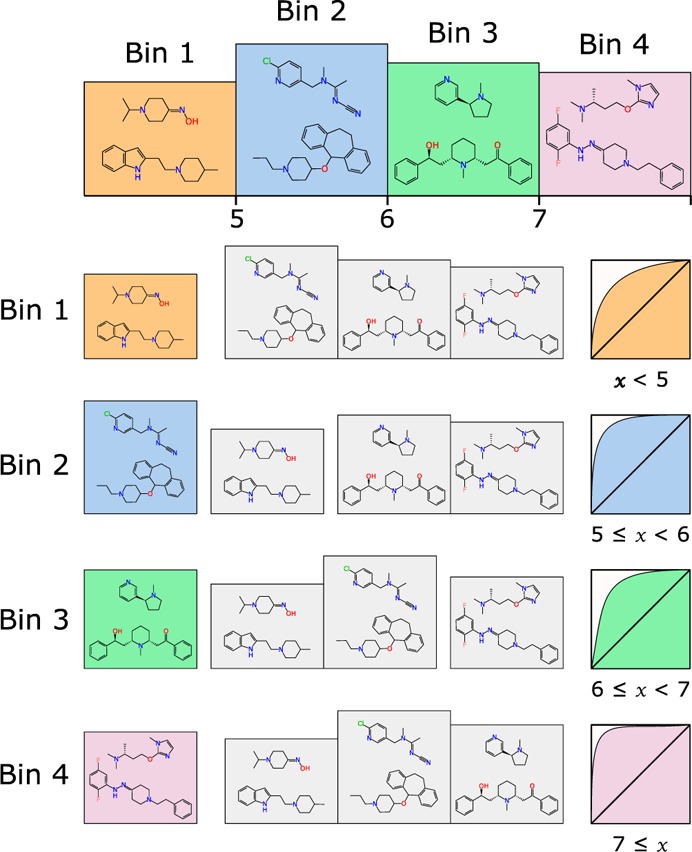
Visual example of the binning system: Four groups of molecular structures are divided according to an activity boundary. For each bin, a conventional two-state Laplacian-corrected naïve Bayesian model is constructed using in bin versus not in bin as the classifier.
By making use of the calibration method that we described previously for converting the Laplacian-modified predictions into a probability-like range (i.e., most in-domain predictions are in the range 0..1),22,27 it is meaningful to compare the prediction values for each of the bins. For a proposed molecular structure, the Bayesian model for each bin is applied. The most rudimentary interpretation is that the bin whose model provides the highest calibrated prediction value is the most probable range.
During our initial experimentation with this approach, we found that the success rate for recalling the correct bin was extremely sensitive to the choice of boundary positions separating the bins. Using a convenient scheme (e.g., whole numbers), or selecting bins based on evenly sized proportions, produced results that were very inconsistent, i.e., minor changes in selection of boundaries had a major impact on the rate at which the models were able to predict the correct bin. This is an intuitively justifiable observation since the fundamental prerequisite of a database of structures and activity measurements is that certain structural fragments are correlated with positive or negative trends in activity. If a cluster of compounds with similar activity values and a similar ensemble of significant structural fragments is arbitrarily segregated by a boundary partition drawn through the cluster, one would expect poor results. Consider the schematic shown in Figure 2; the graph shows a histogram of frequency plotted against activity, for which the compounds are divided into three groups. Representative structures from each of these groups are shown, and each can be clearly seen to have their own distinctive structural characteristics. In this contrived example, the solution is obvious; the data set should be partitioned into three bins, and the boundaries denoted by the heavy green lines show the optimum partitioning. If one were to choose a partitioning scheme that balances the bin sizes evenly, creating three equally proportioned bins would cause the partitions to be drawn through clusters of distinct structure–activity groups. Proceeding with this suboptimal partitioning would be expected to lead to generally poor results because the ability of any model to distinguish between two structures that are very similar but have been classified differently due to miniscule differences in activity will be poor. Similarly unsophisticated approaches, such as setting boundaries by using round numbers (e.g., [4, 8] or [3, 6, 9]), leads to inconsistent results for the same reason.
Figure 2.
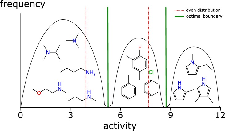
Demonstration of separation of structure activity groups by population integral (red line) or by boundaries between different categories of structure–activity relationships (green line).
To solve this problem it is necessary to compose a method for identifying suitable boundary points that distinguish between clusters of structure–activity relationships. In general, this is not straightforward since model building exercises can be expected to encounter widely diverging scenarios. In some cases, clusters of structures with similar composition and similar activity are encountered, i.e., as shown in Figure 2, but many data sets have much more amorphous relationships between structural fragments and activity. There are of course many real world experimental data sets that have essentially no structure–activity relationship, meaning that a treatment with structure-derived fingerprints like ECFP6 is unlikely to elucidate any correlation better than noise.
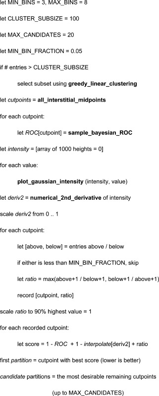
As mentioned in the introduction, a further constraint of the requirements for the method is that it has to function as a “black box” in that the user provides a collection of structures and activities and is not required to provide any further parameters or even have any prior knowledge of the content or whether it is even suitable for modeling. The method we have developed involves proposing a series of candidate cut points that might be used to divide bins, and each of them is scored by criteria such as the relative sizes of the new bins that it would create and how well a test-model would be able to predict which side of the threshold the newly separated molecules reside. The scores are made up of three components: (1) ROC integral from the trial Bayesian model, (2) second derivative of the activity population, and (3) ratio of actives vs inactives. Each of these terms are used in a way that encourages splitting the data set at points that distinctively segregate boundaries between structure–activity groups.
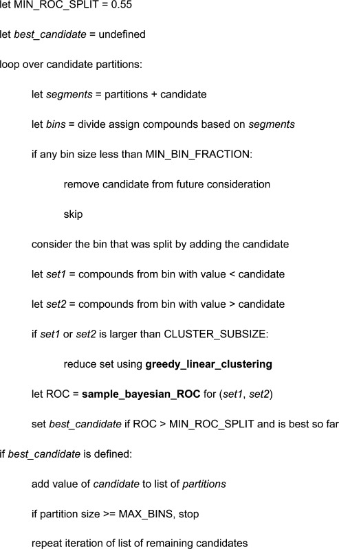
The method is iterative and greedy, starting by dividing the data into two bins, and continuing on to subdivide bins until no more favorable opportunities exist.
Detection of the partitioning boundaries is performed using the following steps:
In this way, each of the putative boundaries (cut points) that has a reasonable balance of entries above and below is recorded and assigned an initial desirability score. The algorithms referred to in bold are summarized only briefly and can be examined in more detail in the source code (http://github.com/cdd/bayseg):
-
•
greedy_linear_clustering: If the list of compounds exceeds a maximum count, the ECFP6 fingerprints are used to reduce the size to the given count in a way that maximizes diversity of structural features and diversity of activity values, while also running in O(N) time for large data sets.
-
•
all_interstitial_midpoints: The list of activity values is sorted, and for each adjacent pair of nonequal values, the midpoint is retained.
-
•
sample_bayesian_ROC: A Bayesian model is created from the list of compounds where activity is based on being above/below the putative threshold, and the receiver-operator-characteristic (ROC) integral is returned; this is fast because fingerprints are already calculated and the collection is guaranteed to be small.
-
•
plot_gaussian_intensity: An array of values is defined, which represents an evenly sampled distribution from lowest to highest activity, plus an edge buffer; for each value, a Gaussian distribution is added to the entire array, resulting in a smooth/smeared out frequency histogram.
-
•
numerical_2nd_derivative: The intensity array is differentiated twice numerically by setting each value to the difference between its two neighbors.
After these scores are calculated, the cut point that is most desirable (lowest score) is recorded and used as the first partition. The remaining cut points are sorted and enumerated, and this list is used in the following section, which iteratively adds additional partition boundaries:
The iterative addition of new partition boundaries stops when the process runs out of candidates or the maximum limit is encountered. The iterative addition is greedy; at each step, it attempts to add a new cut point in the midst of an existing partition in a way that best separates the partition, from a model building point of view. Each iteration involves going through all of the candidates and all of the bins, which is in itself O(N2), but since the number of bins is small and capped and the list of candidates is initially capped and consists of only cut points that were considered desirable for applying to the data overall, the total number of evaluations is never more than hundreds, depending on the parameters and the properties of the incoming data set. For large data sets, the process of creating a Bayesian model for each iteration is kept brief by using the greedy linear clustering method, which is fast and O(N).
As mentioned in the Introduction, the process of selecting good partition boundaries is by far the most difficult part of the method since the remaining steps can be composed from existing methods for working with Bayesian models. The objective is to create a model for each bin such that for any proposed compound the model that gives the highest prediction is that which corresponds to the range of activities that includes the actual activity for the compound.
In our previous article,22 we described a method for post-calibrating the Laplacian-corrected naïve Bayesian models that are effective for structure-derived fingerprint-based models, so that the results of each prediction are probability-like. This calibration is done by analyzing the ROC curve and is used to transform the numeric results so that most predictions within the domain of the model fall between the range 0..1, which means that they can be independently interpreted. It also means that these calibrated results can be compared between models, and therefore, it is reasonable to expect that for two mutually exclusive models the one that produces the higher value can be considered the leading contender. The extent to which this hypothesis holds true is described in the Results section.
For conventional binary Bayesian models, the method of choice for evaluating structure–activity relationships is the venerable receiver-operator-characteristic (ROC) curve, which can be neatly summarized by its integral. This does not apply to the composite models, and instead, a different set of visual and quantitative metrics is needed. The primary objective is for all models to predict the correct bin by ensuring that its corresponding model produces the highest value, and so the fraction of the time for which compounds in a training set accomplish this is relevant, relative to the chance of guessing randomly. For example, a composite model with five bins might presume that a random guess would be correct 20% of the time, and hence, if the model predicts the correct bin 60% of the time, this represents a 3× improvement. For simplicity purposes, it is assumed that no prior knowledge of the bin distribution of the training set is available, and hence, each bin is equally likely to be guessed correctly. It is also assumed that the bin sizes are approximately the same in terms of membership frequency, which is reasonable since the detection method ensures that the training set is partitioned so that no one bin represents a disproportionate fraction of the training set. For increasingly large bin counts, the consolation prize for predicting the adjacent bin (off-by-1) becomes more useful, and so it is relevant to provide more information than just the “direct hits”.
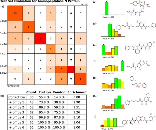
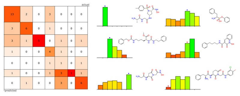
Figure 3 shows some of the results obtained by evaluating the test set for a composite model of aminopeptidase-N inhibitor candidates (extracted from ChEMBL v2022,33,34). The response matrix for the test set is shown in (a); as can be seen quickly with the chosen visual style, the majority of predicted responses are concentrated along the diagonal, which corresponds to correct prediction of bins. The off-diagonal cells correspond to predictions that were incorrect. The table in (b) provides summary details; the first row indicates that 55.4% of the test set entries were predicted to be in the correct bin. Since there are seven bins, a random guess would have a 14.3% chance of being correct if an even distribution is assumed, and so the composite model provides an enrichment factor of 3.88. The next row in the table expands the definition of success to include results that were predicted to be in the adjacent bin, for which 73.8% of results qualify, relative to a random chance of 38.8%. Subsequent rows in the table converge to 100% as the bar is lowered.
Figure 3.
Example of a data set containing activities against aminopeptidase N-protein with 651 measurements, of which 65 were reserved for use in the training set. The correctness matrix is shown in (a), while (b) shows enrichment statistics, and (c–i) show examples of molecular predictions from the test set.
On the right-hand side of Figure 3 are a number of visual representations of individual predictions for selected molecules from the test set. In each case a series of seven bars are shown, and these are assigned height and color-coding in proportion to the calibrated prediction of the underlying model. The highest (and most green-tinted) bar is taken to be the predicted bin of choice for bulk evaluation purposes, but for evaluation of a small number of prospective molecules, it is useful to provide all of this information in a visually accessible way, so that the user can make a more informed judgment about the value of the model prediction.
The most definitive example is shown in Figure 3c, for which a single bin corresponds to a very high prediction, and the other six are essentially zero. As it happens, the molecular structure contains a hydroxyamide functional group, which is unique within the training and test sets and represents an overwhelmingly dominant structure–activity trend. The example in Figure 3d is quite definitive, with one prediction—the correct one—standing out, but with nonzero predictions for several other bins. The cases shown for Figure 3e–g all predict the correct bin, but there are patterns of competing structure–activity relationship that make other options quite plausible and hence might be thought of skeptically. For case Figure 3h, the correct result is marked by a red dot above the bar, which does not correspond to the highest prediction; however, it can be seen that the model is working quite well and hit the adjacent bin by a moderate margin. Case Figure 3i, on the other hand, shows a poor result, where the actual activity is in the lowest category, but the intermediate level models showed quite high predictions.
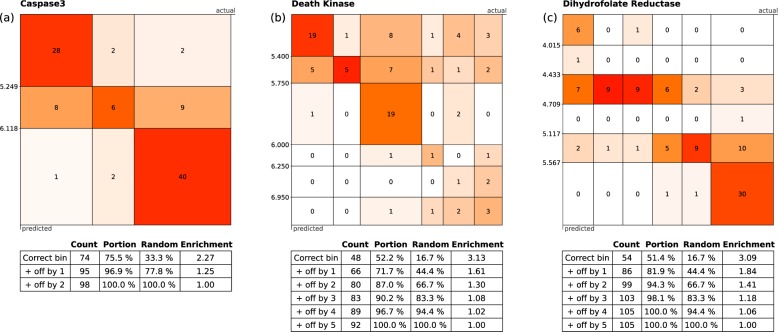
Figure 4 shows three response matrices for selected data sets (Caspase3, Death kinase, and dihydrofolate reductase), also extracted from ChEMBL v20. In Figure 4a, the Caspase3 distribution was resolved into only three distinct bins. While the models performed well and the correct prediction rate for the test set was 75.5%, the enrichment rate is only 2.27 since the chance of randomly guessing the correct bin is 1 in 3. The other two examples, Figure 4b and c, were divided into six bins, and both indicate a respectable success rate. However, the rate of correct prediction for each of the bins is quite variable. While there is significant opportunity for random error when using a small test set, an abnormally low success rate for a particular bin tends to be indicative of the inability to extract a meaningful structure–activity relationship for the compounds within the bin using Bayesian methods and ECFP6 fingerprints.
Figure 4.
Three examples of recall rates: (a) Caspase (980 rows), (b) Death kinase (926 rows), and (c) dihydrofolate reductase (1056 rows). In each case, 10% of the structures were retained for use as the testing set.
Results
In order to determine the boundaries of performance with composite models using real data, we applied the method to a selection of 1843 data sets, extracted from ChEMBL v 20,33,34 using a method similar to that which we described previously.22 Each of the models contained at least 100 structure–activity data points assigned to the same target and consisted of either Ki or IC50 type measurements but not both. The validation data sets were not filtered in any way by the presence or absence of an actual structure–activity relationship, and so it can be expected that some proportion of the data sets are simply not suited to modeling. We consider it reasonable to operate under the assumption that the data sets extracted from ChEMBL are representative of the kinds of real world drug discovery scenarios for which this method will be used. The collection of structures and activities that were used for this validation exercise can be downloaded from http://www.collaborativedrug.com/composite-bayes.32
For each data set, 10% of the entries were set aside to use as the test set. These entries were selected using the greedy clustering algorithm described earlier, which means that in general the choice of test set is nondiabolical and falls within the same domain as the training set (although it should be noted that when we repeated the experiment with a random selection of testing sets there was no bias in favor of preclustering). Data sets for which the partition detection method was not able to detect at least three bins were left out of the results.
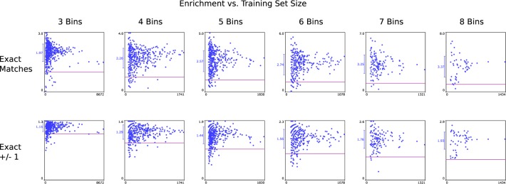
Figure 5 shows the distribution of results, where the percentage of successful prediction of compounds within the testing set is plotted against the size of the data set. The first row shows the enrichment rate of correct detection for each of the bin sizes from 3 through 8. In each case, a horizontal purple line shows an enrichment rate of 1, which corresponds to no better than random. The average and standard deviation is indicated to the left of the vertical axis. As shown, the large majority of data sets demonstrate substantial predictive power relative to random guessing. As the size of the data set grows, the enrichment rate converges toward the overall average, which indicates that larger data sets are less prone to random fluctuations.
Figure 5.
Unsupervised model building based on 1843 data sets extracted from ChEMBL v20. Results are divided into bin sizes (columns). Each point corresponds to the ratio of correctly predicted bins versus chance of random guessing (enrichment), with a purple line indicating the null hypothesis. The average and standard deviation are marked on the Y-axis. Training set size is shown on the X-axis. The testing sets were made up of 10% of each total data set.
The second row of graphs in Figure 5 shows the enrichment rate for predictions that indicated either the correct bin or a bin adjacent to the correct bin as the highest performer. While the chance of meeting this criterion by random guessing is increased, especially for smaller bins, the same overall trend is observed.
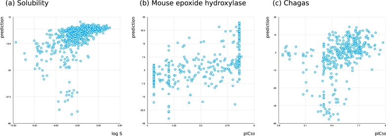
Three data sets were selected for further study: solubility (log S),35 mouse epoxide hydroxylase (mouse, pIC50),32,36−39 and Chagas disease (pIC50).40 In order to establish that the composite models are adding predictive value relative to the much simpler method of correlating the raw prediction values from a single Bayesian model, each of these data sets was partitioned into equally sized training and testing sets (using the greedy linear clustering method, as described above) with the threshold set to the median activity. Figure 6 shows each of the predictions plotted against the actual value, and in each case, the correlation is very poor. This is to be expected since the two-state Bayesian model is quite simply not provided with enough information to distinguish between intermediate predictions.
Figure 6.
Three examples of correlating raw Laplacian-modified naïve Bayesian predictions with activity: (a) solubility (test set = 649, R2 = 0.513), (b) mouse epoxide hydroxylase (test set = 328, R2 = 0.582), and (c) activity against Chagas disease (test set = 371, R2 = 0.393).
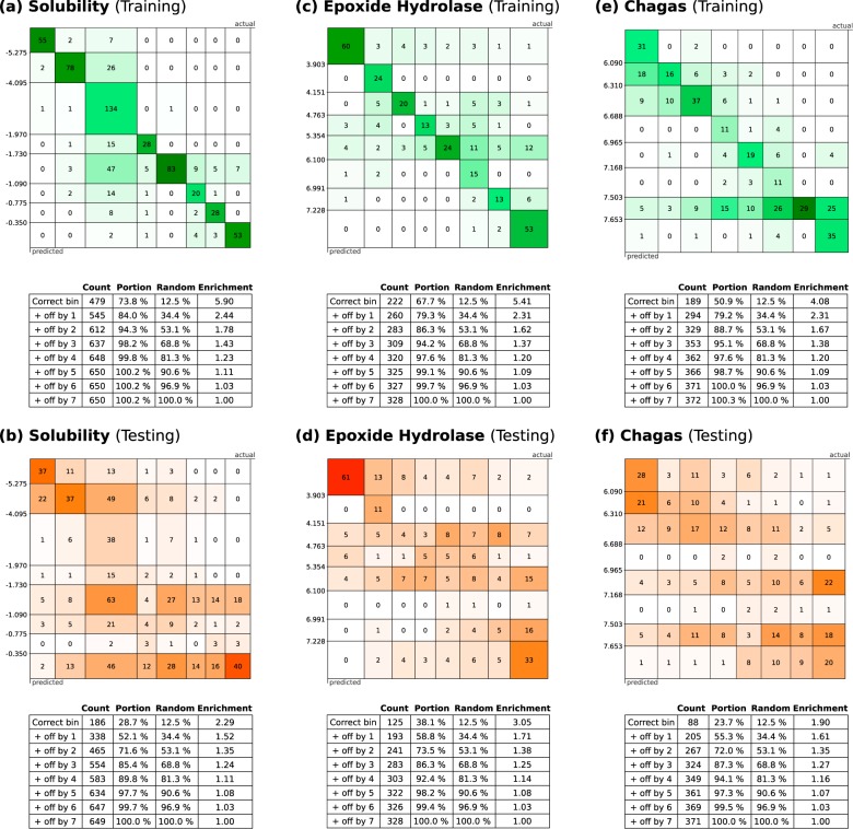
The results for running the composite model method on three selected data sets are shown in Figure 7. The axis positions represent actual vs predicted bins, whereby each occupancy along the diagonal represents an instance where the correct bin had the highest prediction. The grid sizes are scaled so that the area of each cell on the diagonal is proportional to the actual population of the bin. Off-diagonal occupancies show how far and how often the strongest prediction strayed from the correct value. Each cell is color-coded using a shade that is scaled according to the average actual population of the corresponding bins, i.e., diagonal cells are darkest if there are no incorrect predictions, and a pair of off-diagonal cells (i, j) would be darkest if all predictions for either i or j were incorrectly transposed.
Figure 7.
Analysis for three data sets: aqueous solubility, mouse hydrolase epoxide, and Chagas disease. The correctness matrix and enrichment statistics results for the training sets (a, c, e) are shown on the top; test sets are shown below (b, d, f).
The analyses for using the training set data are shown in Figure 7a, c, and e, while the test set predictions are shown in Figure 7b, d, and f. As would be expected, the results for the training set have a much higher recall rate. Nonetheless, the testing set predictions demonstrate substantial enrichment relative to random, and in each case, the correct result ± off by 1 portion is greater than 50%. The effectiveness of the method is largely a function of the extent to which the data set is organized into islands of structure–activity: clusters of molecules with similar structure characteristics and activity values within a distinctive range. The presence of molecules with similar structural features and a wide range of activities spanning multiple groups degrades the ability of the method to prioritize the correct bin as the primary choice, but as shown in Figure 3, the probabilistic results can at least favor a subset of all the available options. The underlying fingerprints (ECFP6) are designed to statistically express explicit structural features, which has the advantage of being highly interpretable by chemists examining the structures, but it should be noted that this is not necessarily the most effective way to capture more abstract features like shape, size, polarity, etc. The ability to resolve effects like bioisosterism is only possible if the applicable patterns are present in the training set.
It is important to think of the composite Bayesian model approach as a solution to a particular use case, rather than an alternative to methods such as QSAR/QSPR41−44 modeling of continuous properties, which it is not intended to displace. As mentioned in the Introduction, the requirements for the method are that the user possess no expertise in modeling, has no preexisting understanding of the structure–activity trends, and is not required to perform any analysis or refinement of the model. The method is required to operate with the user simply uploading a collection of structures and activities and from this provide a way to evaluate proposed structures and gain insight that is qualitatively useful.
Discussion
This study extends the preceding work describing the development of open source Bayesian models.22,27 In addition, it complements earlier efforts to partition training or test sets.22 For example, our recent work on microsomal stability in mouse demonstrated improved binary Bayesian models by “pruning” out the moderately unstable/moderately stable compounds from the training set.45 Earlier work had used a support vector machine to perform novelty detection and margin detection to remove uncertain predictions from models using Kernel–PLS.46 These represent attempts to refine the way we approach using data for test or training sets with Bayesian and other machine learning models.
We have now extended the use case scenario for the popular Laplacian-modified naïve Bayesian method based on ECFP6 fingerprints to include predictions for data sets that are more appropriately divided into multiple categories rather than just two states. In doing so, we have preserved some of the most desirable properties of this Bayesian method, such as requiring little or no expertise on behalf of the user, being quite robust to the effects of over/under-training, producing intuitive results that are closely related to the underlying structure activity relationship, rapid performance on modest computing hardware, and being constructed entirely of open source and easily portable algorithms. We have also made a point of evaluating the method on a huge collection of curated data sets (extracted from ChEMBL v2033,34,47), which is intended to simulate the diversity of data encountered in drug discovery research. Whereby, some collections have a strong and easily identifiable correlation between structural features and activity, while other collections have very little correlation, for a variety of possible reasons (e.g., multiple binding modes, multiple targets, complex biology, low data quality, noise, frequent hitters,48−50 aggregators,51−55 PAINS,56 etc.). These new models can be downloaded at http://www.collaborativedrug.com/composite-bayes. The large majority of data sets demonstrate substantial predictive power relative to random. As the size of the data set grows, the enrichment rate converges toward the overall average (as is demonstrated in Figure 5), which suggests that larger data sets are less prone to random fluctuations.
Three additional data sets were studied with the composite Bayesian model approach: solubility,35 epoxide hydrolase,32,36−39 and Chagas disease.40 While conventional two-state Bayesian modeling can be used to some effect on these data sets (as we have previously described22,27,40), the classification of all molecules into two categories is a blunt instrument and is generally ineffective at predicting intermediate responses. The process of bin assignment followed by composite model generation provides more degrees of freedom for structure features to be associated with finer grained activity levels. Whether this is the appropriate method for the data set, i.e., multiple groups of structure–activity correlations actually exist, can be evaluated by the quality of the metrics returned by the method. The enrichment value for correctly predicted bins from within the training set can also be used as a top level indication of model quality, much like ROC values are used for conventional Bayesian models. While they do not tell the whole story, they do convey a significant amount of information about the likely effectiveness of the model building exercise, and low values definitively indicate poor results from this modeling technique.
Machine learning approaches have found wide applications in numerous areas such as genetics and genomics57 (e.g., predicting multiple cancer classes58). The Bayesian classifier approach has also been used widely in cheminformatics for target prediction where there are multiple classes/targets.59−64 The composite Bayesian model approach that we have described should be considered as an extension of the two-state Bayesian method rather than a replacement for prediction of continuous properties by conventional QSAR/QSPR methods, as the outcome is probabilistic in nature rather than an attempt to simulate an experimental measurement, complete with error bars.
The composite Bayesian method described has been made available as open source (http://github.com/cdd/bayseg) along with the corresponding validation materials. We are currently creating a user interface that fits within the CDD Models(27) extension to the CDD Vault(65,66) service, and we intend to bring this additional form of structure–activity modeling to nonexpert users in this commercial software, much as we did when the binary Bayesian modeling was implemented in the same software. Because the composite Bayesian method is designed for unsupervised use, we will be able to design the functionality in such a way that the user is taken directly to the results of the model building rather than having to setup various model parameters and iteratively examine their effectiveness. We will also apply variations of the methods described in this article for making an automated determination of whether a data set is more appropriate for binary Bayesian modeling or for the multistate composite Bayesian method.
The composite model technique that we have described is comprised of two distinct steps: selecting the partitions and modeling them competitively. While we have applied the same set of Bayesian/ECFP6 technologies to solve both of these problems, it may well be productive to explore other techniques for scoring molecules for membership within these bins (such as other machine learning methods). The use of sampled Bayesian models to detect boundary thresholds and separate groups of structure–activity relationships is effective and has desirable properties (e.g., performance, unit agnostic), but methods such as QSAR/QSPR may turn out to be more effective for scoring the resulting bins. In future work, we intend to investigate such methods, as it may well be possible to deliver improved predictions while still adhering to the same use-case constraints, namely, zero user input.
In conclusion, while much has been published on the use of Bayesian models in cheminformatics,67 we have now developed an approach (which to our knowledge has not been addressed before) that may extend them further, making them potentially more useful, when further granularity is required. The advantages of this approach are that it is fast, designed for use without operator intervention, easily implemented, and open source.
Acknowledgments
We gratefully acknowledge Dr. Barry Bunin and all our colleagues at CDD for their support and development of CDD Models. This project was supported by Award Number 9R44TR000942-02 “Biocomputation across distributed private datasets to enhance drug discovery” from the NIH National Center for Advancing Translational Sciences. The Chagas disease dataset was collected and used with funding from NIH National Institute of Allergy and Infectious Diseases grant R41-AI108003-01 “Identification and validation of targets of phenotypic high throughput screening”. Source code for the methods described and example data sets used for the figures can be found in Github (http://github.com/cdd/bayseg) and leverages our previous contributions to the Chemical Development Kit (CDK), version 1.5.11. Extracts from ChEMBL v20 used for large-scale validation can be downloaded from Collaborative Drug Discovery (http://www.collaborativedrug.com/composite-bayes).
Glossary
Abbreviations Used:
- ADME/Tox
Absorption, Distribution, Metabolism, Excretion and Toxicity
- CDD
Collaborative Drug Discovery
- CDK
Chemistry Development Toolkit
- ECFP6
Extended Connectivity Fingerprints of maximum diameter 6
- FCFP6
molecular Function Class Fingerprints of maximum diameter 6
- HTS
High Throughput Screens
- LGPL
Lesser Gnu Public License
- QSAR
Quantitative Structure–Activity Relationships
- QSPR
Quantitative Structure–Property Relationship
- ROC
Receiver-Operator-Curve
Author Contributions
A.M.C. and K.D. developed the software, and S.E. provided data sets. All authors co-wrote the manuscript.
The authors declare the following competing financial interests: S.E. is a consultant for Collaborative Drug Discovery, Inc. A.M.C. is the founder of Molecular Materials Informatics, Inc.
References
- Litterman N. K.; Lipinski C. A.; Bunin B. A.; Ekins S. Computational Prediction and Validation of an Expert’s Evaluation of Chemical Probes. J. Chem. Inf. Model. 2014, 54, 2996–3004. 10.1021/ci500445u. [DOI] [PMC free article] [PubMed] [Google Scholar]
- Ekins S.; Pottorf R.; Reynolds R. C.; Williams A. J.; Clark A. M.; Freundlich J. S. Looking back to the future: predicting in vivo efficacy of small molecules versus Mycobacterium tuberculosis. J. Chem. Inf. Model. 2014, 54, 1070–82. 10.1021/ci500077v. [DOI] [PMC free article] [PubMed] [Google Scholar]
- Ekins S.; Freundlich J. S.; Reynolds R. C. Are Bigger Data Sets Better for Machine Learning? Fusing Single-Point and Dual-Event Dose Response Data for Mycobacterium tuberculosis. J. Chem. Inf. Model. 2014, 54, 2157–65. 10.1021/ci500264r. [DOI] [PMC free article] [PubMed] [Google Scholar]
- Ekins S.; Freundlich J. S.; Hobrath J. V.; Lucile White E.; Reynolds R. C. Combining computational methods for hit to lead optimization in Mycobacterium tuberculosis drug discovery. Pharm. Res. 2014, 31, 414–35. 10.1007/s11095-013-1172-7. [DOI] [PMC free article] [PubMed] [Google Scholar]
- Ekins S.; Casey A. C.; Roberts D.; Parish T.; Bunin B. A. Bayesian models for screening and TB Mobile for target inference with Mycobacterium tuberculosis. Tuberculosis (Oxford, U. K.) 2014, 94, 162–9. 10.1016/j.tube.2013.12.001. [DOI] [PMC free article] [PubMed] [Google Scholar]
- Ekins S. Progress in computational toxicology. J. Pharmacol. Toxicol. Methods 2014, 69, 115–40. 10.1016/j.vascn.2013.12.003. [DOI] [PubMed] [Google Scholar]
- Ekins S.; Reynolds R. C.; Franzblau S. G.; Wan B.; Freundlich J. S.; Bunin B. A. Enhancing Hit Identification in Mycobacterium tuberculosis Drug Discovery Using Validated Dual-Event Bayesian Models. PLoS One 2013, 8, e63240. 10.1371/journal.pone.0063240. [DOI] [PMC free article] [PubMed] [Google Scholar]
- Ekins S.; Reynolds R.; Kim H.; Koo M.-S.; Ekonomidis M.; Talaue M.; Paget S. D.; Woolhiser L. K.; Lenaerts A. J.; Bunin B. A.; Connell N.; Freundlich J. S. Bayesian Models Leveraging Bioactivity and Cytotoxicity Information for Drug Discovery. Chem. Biol. 2013, 20, 370–378. 10.1016/j.chembiol.2013.01.011. [DOI] [PMC free article] [PubMed] [Google Scholar]
- Dong Z.; Ekins S.; Polli J. E. Structure-activity relationship for FDA approved drugs as inhibitors of the human sodium taurocholate cotransporting polypeptide (NTCP). Mol. Pharmaceutics 2013, 10, 1008–19. 10.1021/mp300453k. [DOI] [PMC free article] [PubMed] [Google Scholar]
- Astorga B.; Ekins S.; Morales M.; Wright S. H. Molecular Determinants of Ligand Selectivity for the Human Multidrug And Toxin Extrusion Proteins, MATE1 and MATE-2K. J. Pharmacol. Exp. Ther. 2012, 341, 743–55. 10.1124/jpet.112.191577. [DOI] [PMC free article] [PubMed] [Google Scholar]
- Pan Y.; Li L.; Kim G.; Ekins S.; Wang H.; Swaan P. W. Identification and Validation of Novel hPXR Activators Amongst Prescribed Drugs via Ligand-Based Virtual Screening. Drug Metab. Dispos. 2011, 39, 337–344. 10.1124/dmd.110.035808. [DOI] [PMC free article] [PubMed] [Google Scholar]
- Zientek M.; Stoner C.; Ayscue R.; Klug-McLeod J.; Jiang Y.; West M.; Collins C.; Ekins S. Integrated in silico-in vitro strategy for addressing cytochrome P450 3A4 time-dependent inhibition. Chem. Res. Toxicol. 2010, 23, 664–76. 10.1021/tx900417f. [DOI] [PubMed] [Google Scholar]
- Ekins S.; Williams A. J.; Xu J. J. A Predictive Ligand-Based Bayesian Model for Human Drug Induced Liver Injury. Drug Metab. Dispos. 2010, 38, 2302–2308. 10.1124/dmd.110.035113. [DOI] [PubMed] [Google Scholar]
- Diao L.; Ekins S.; Polli J. E. Quantitative Structure Activity Relationship for Inhibition of Human Organic Cation/Carnitine Transporter. Mol. Pharmaceutics 2010, 7, 2120–2130. 10.1021/mp100226q. [DOI] [PMC free article] [PubMed] [Google Scholar]
- Zheng X.; Ekins S.; Raufman J. P.; Polli J. E. Computational models for drug inhibition of the human apical sodium-dependent bile acid transporter. Mol. Pharmaceutics 2009, 6, 1591–603. 10.1021/mp900163d. [DOI] [PMC free article] [PubMed] [Google Scholar]
- Ekins S.; Kortagere S.; Iyer M.; Reschly E. J.; Lill M. A.; Redinbo M. R.; Krasowski M. D. Challenges predicting ligand-receptor interactions of promiscuous proteins: the nuclear receptor PXR. PLoS Comput. Biol. 2009, 5, e1000594. 10.1371/journal.pcbi.1000594. [DOI] [PMC free article] [PubMed] [Google Scholar]
- Klon A. E.; Lowrie J. F.; Diller D. J. Improved naive Bayesian modeling of numerical data for absorption, distribution, metabolism and excretion (ADME) property prediction. J. Chem. Inf. Model. 2006, 46, 1945–56. 10.1021/ci0601315. [DOI] [PubMed] [Google Scholar]
- Rogers D.; Brown R. D.; Hahn M. Using extended-connectivity fingerprints with Laplacian-modified Bayesian analysis in high-throughput screening follow-up. J. Biomol. Screening 2005, 10, 682–6. 10.1177/1087057105281365. [DOI] [PubMed] [Google Scholar]
- Chen B.; Sheridan R. P.; Hornak V.; Voigt J. H. Comparison of random forest and Pipeline Pilot Naive Bayes in prospective QSAR predictions. J. Chem. Inf. Model. 2012, 52, 792–803. 10.1021/ci200615h. [DOI] [PubMed] [Google Scholar]
- Mussa H. Y.; Marcus D.; Mitchell J. B.; Glen R. C. Verifying the fully ″Laplacianised″ posterior Naive Bayesian approach and more. J. Cheminf. 2015, 7, 27. 10.1186/s13321-015-0075-5. [DOI] [PMC free article] [PubMed] [Google Scholar]
- Mussa H. Y.; Mitchell J. B.; Glen R. C. Full ″Laplacianised″ posterior naive Bayesian algorithm. J. Cheminf. 2013, 5, 37. 10.1186/1758-2946-5-37. [DOI] [PMC free article] [PubMed] [Google Scholar]
- Clark A. M.; Ekins S. Open Source Bayesian Models: 2. Mining A ″big dataset″ to create and validate models with ChEMBL. J. Chem. Inf. Model. 2015, 55, 1246–1260. 10.1021/acs.jcim.5b00144. [DOI] [PubMed] [Google Scholar]
- Dearden J. C.; Cronin M. T.; Kaiser K. L. How not to develop a quantitative structure-activity or structure-property relationship (QSAR/QSPR). SAR QSAR Environ. Res. 2009, 20, 241–66. 10.1080/10629360902949567. [DOI] [PubMed] [Google Scholar]
- Stanton D. T.; Mattioni B. E.; Knittel J. J.; Jurs P. C. Development and use of hydrophobic surface area (HSA) descriptors for computer-assisted quantitative structure-activity and structure-property relationship studies. J. Chem. Inf. Model. 2004, 44, 1010–23. 10.1021/ci034284t. [DOI] [PubMed] [Google Scholar]
- Taboureau O. Methods for building quantitative structure-activity relationship (QSAR) descriptors and predictive models for computer-aided design of antimicrobial peptides. Methods Mol. Biol. 2010, 618, 77–86. 10.1007/978-1-60761-594-1_6. [DOI] [PubMed] [Google Scholar]
- Esposito E. X.; Hopfinger A. J.; Madura J. D. Methods for applying the quantitative structure-activity relationship paradigm. Methods Mol. Biol. 2004, 275, 131–214. 10.1385/1-59259-802-1:131. [DOI] [PubMed] [Google Scholar]
- Clark A. M.; Dole K.; Coulon-Spektor A.; McNutt A.; Grass G.; Freundlich J. S.; Reynolds R. C.; Ekins S. Open source bayesian models: 1. Application to ADME/Tox and drug discovery datasets. J. Chem. Inf. Model. 2015, 55, 1231–1245. 10.1021/acs.jcim.5b00143. [DOI] [PMC free article] [PubMed] [Google Scholar]
- Ekins S.; Freundlich J. S.; Reynolds R. C. Fusing dual-event datasets for Mycobacterium Tuberculosis machine learning models and their evaluation. J. Chem. Inf. Model. 2013, 53, 3054–63. 10.1021/ci400480s. [DOI] [PMC free article] [PubMed] [Google Scholar]
- Ekins S.; Freundlich J. S. Validating new tuberculosis computational models with public whole cell screening aerobic activity datasets. Pharm. Res. 2011, 28, 1859–69. 10.1007/s11095-011-0413-x. [DOI] [PubMed] [Google Scholar]
- Ekins S.; Kaneko T.; Lipinski C. A.; Bradford J.; Dole K.; Spektor A.; Gregory K.; Blondeau D.; Ernst S.; Yang J.; Goncharoff N.; Hohman M.; Bunin B. Analysis and hit filtering of a very large library of compounds screened against Mycobacterium tuberculosis. Mol. BioSyst. 2010, 6, 2316–2324. 10.1039/c0mb00104j. [DOI] [PubMed] [Google Scholar]
- Ekins S.; Bradford J.; Dole K.; Spektor A.; Gregory K.; Blondeau D.; Hohman M.; Bunin B. A Collaborative Database And Computational Models For Tuberculosis Drug Discovery. Mol. BioSyst. 2010, 6, 840–851. 10.1039/b917766c. [DOI] [PubMed] [Google Scholar]
- CSS Public Access. https://www.collaborativedrug.com/pages/public_access (accesed January 2016).
- Papadatos G.; Overington J. P. The ChEMBL database: a taster for medicinal chemists. Future Med. Chem. 2014, 6, 361–4. 10.4155/fmc.14.8. [DOI] [PubMed] [Google Scholar]
- Gaulton A.; Bellis L. J.; Bento A. P.; Chambers J.; Davies M.; Hersey A.; Light Y.; McGlinchey S.; Michalovich D.; Al-Lazikani B.; Overington J. P. ChEMBL: a large-scale bioactivity database for drug discovery. Nucleic Acids Res. 2012, 40, D1100–7. 10.1093/nar/gkr777. [DOI] [PMC free article] [PubMed] [Google Scholar]
- Huuskonen J. Estimation of aqueous solubility for a diverse set of organic compounds based on molecular topology. J. Chem. Inf. Model. 2000, 40, 773–7. 10.1021/ci9901338. [DOI] [PubMed] [Google Scholar]
- McElroy N. R.; Jurs P. C.; Morisseau C.; Hammock B. D. QSAR and classification of murine and human epoxide hydrolase inhibition by urea-like compounds. J. Med. Chem. 2003, 46, 1066–1080. 10.1021/jm020269o. [DOI] [PubMed] [Google Scholar]
- Nakagawa Y.; Wheelock C. E.; Morisseau C.; Goodrow M. H.; Hammock B. G.; Hammock B. D. 3D-QSAR analysis of inhibition of murine soluble epoxide hydrolase (MsEH) by benzoylureas, arylureas, and their analogues. Bioorg. Med. Chem. 2000, 8, 2663–2673. 10.1016/S0968-0896(00)00198-X. [DOI] [PubMed] [Google Scholar]
- Argiriadi M. A.; Morisseau C.; Goodrow M. H.; Dowdy D. L.; Hammock B. D.; Christianson D. W. Binding of the alkylurea inhibitors to epoxide hydrolase implicates active site tyrosines in substrate activation. J. Biol. Chem. 2000, 275, 15265–15270. 10.1074/jbc.M000278200. [DOI] [PubMed] [Google Scholar]
- Morisseau C.; Du G.; Newman J. W.; Hammock B. D. Mechanism of mammalian soluble epoxide hydrolase inhibition by chalcone oxide derivatives. Arch. Biochem. Biophys. 1998, 356, 214–228. 10.1006/abbi.1998.0756. [DOI] [PubMed] [Google Scholar]
- Ekins S.; Lage de Siqueira-Neto J.; McCall L.-I.; Sarker M.; Yadav M.; Ponder E. L.; Kallel E. A.; Kellar D.; Chen S.; Arkin M.; Bunin B. A.; McKerrow J. H.; Talcott C. Machine Learning Models and Pathway Genome Data Base for Trypanosoma cruzi Drug Discovery. PLoS Neglected Trop. Dis. 2015, 9, e0003878. 10.1371/journal.pntd.0003878. [DOI] [PMC free article] [PubMed] [Google Scholar]
- Kubinyi H.; Folkers G.; Martin Y. C.. 3D-QSAR in Drug Design; Kluwer/ESCOM: Leiden, 1998. [Google Scholar]
- Kubinyi H. QSAR and 3D QSAR in drug design Part 2: applications and problems. Drug Discovery Today 1997, 2, 538–546. 10.1016/S1359-6446(97)01084-2. [DOI] [Google Scholar]
- Kubinyi H. QSAR and 3D QSAR in drug design Part1: methodology. Drug Discovery Today 1997, 2, 457–467. 10.1016/S1359-6446(97)01079-9. [DOI] [Google Scholar]
- Kortagere S.; Ekins S. Troubleshooting computational methods in drug discovery. J. Pharmacol. Toxicol. Methods 2010, 61, 67–75. 10.1016/j.vascn.2010.02.005. [DOI] [PubMed] [Google Scholar]
- Perryman A. L.; Stratton T. P.; Ekins S.; Freundlich J. S. Predicting mouse liver microsomal stability with "pruned" machine learning models and public data. Pharm. Res. 2016, 33, 433–49. 10.1007/s11095-015-1800-5. [DOI] [PMC free article] [PubMed] [Google Scholar]
- Ekins S.; Embrechts M. J.; Breneman C. M.; Jim K.; Wery J.-P.. Novel Applications of Kernel-Partial Least Squares to Modeling a Comprehensive Array of Properties for Drug Discovery. In Computational Toxicology: Risk Assessment for Pharmaceutical and Environmental Chemicals, Ekins S., Ed.; Wiley-Interscience: Hoboken, NJ, 2007; pp 403–432. [Google Scholar]
- Bento A. P.; Gaulton A.; Hersey A.; Bellis L. J.; Chambers J.; Davies M.; Kruger F. A.; Light Y.; Mak L.; McGlinchey S.; Nowotka M.; Papadatos G.; Santos R.; Overington J. P. The ChEMBL bioactivity database: an update. Nucleic Acids Res. 2014, 42, D1083–90. 10.1093/nar/gkt1031. [DOI] [PMC free article] [PubMed] [Google Scholar]
- Bender A.; Mikhailov D.; Glick M.; Scheiber J.; Davies J. W.; Cleaver S.; Marshall S.; Tallarico J. A.; Harrington E.; Cornella-Taracido I.; Jenkins J. L. Use of ligand based models for protein domains to predict novel molecular targets and applications to triage affinity chromatography data. J. Proteome Res. 2009, 8, 2575–85. 10.1021/pr900107z. [DOI] [PubMed] [Google Scholar]
- Crisman T. J.; Parker C. N.; Jenkins J. L.; Scheiber J.; Thoma M.; Kang Z. B.; Kim R.; Bender A.; Nettles J. H.; Davies J. W.; Glick M. Understanding false positives in reporter gene assays: in silico chemogenomics approaches to prioritize cell-based HTS data. J. Chem. Inf. Model. 2007, 47, 1319–27. 10.1021/ci6005504. [DOI] [PubMed] [Google Scholar]
- Roche O.; Schneider P.; Zuegge J.; Guba W.; Kansy M.; Alanine A.; Bleicher K.; Danel F.; Gutknecht E.-M.; Rogers-Evans M.; Neidhart W.; Stalder H.; Dillon M.; Sjogren E.; Fotouhi N.; Gillespie P.; Goodnow R.; Harris W.; Jones P.; Taniguchi M.; Tsujii S.; von der saal W.; Zimmermann G.; Schneider G. Development of a virtual screening method for identification of ″frequent hitters″ in compound libraries. J. Med. Chem. 2002, 45, 137–142. 10.1021/jm010934d. [DOI] [PubMed] [Google Scholar]
- Sassano M. F.; Doak A. K.; Roth B. L.; Shoichet B. K. Colloidal aggregation causes inhibition of G protein-coupled receptors. J. Med. Chem. 2013, 56, 2406–14. 10.1021/jm301749y. [DOI] [PMC free article] [PubMed] [Google Scholar]
- Feng B. Y.; Simeonov A.; Jadhav A.; Babaoglu K.; Inglese J.; Shoichet B. K.; Austin C. P. A high-throughput screen for aggregation-based inhibition in a large compound library. J. Med. Chem. 2007, 50, 2385–90. 10.1021/jm061317y. [DOI] [PubMed] [Google Scholar]
- Seidler J.; McGovern S. L.; Doman T. N.; Shoichet B. K. Identification and prediction of promiscuous aggregating inhibitors among known drugs. J. Med. Chem. 2003, 46, 4477–4486. 10.1021/jm030191r. [DOI] [PubMed] [Google Scholar]
- McGovern S. L.; Shoichet B. K. Kinase inhibitors: not just for kinases anymore. J. Med. Chem. 2003, 46, 1478–1483. 10.1021/jm020427b. [DOI] [PubMed] [Google Scholar]
- McGovern S. L.; Caselli E.; Grigorieff N.; Shoichet B. K. A common mechanism underlying promiscuous inhibitors from virtual and high-throughput screening. J. Med. Chem. 2002, 45, 1712–1722. 10.1021/jm010533y. [DOI] [PubMed] [Google Scholar]
- Baell J. B.; Holloway G. A. New Substructure Filters for Removal of Pan Assay Interference Compounds (PAINS) from Screening Libraries and for Their Exclusion in Bioassays. J. Med. Chem. 2010, 53, 2719–2740. 10.1021/jm901137j. [DOI] [PubMed] [Google Scholar]
- Libbrecht M. W.; Noble W. S. Machine learning applications in genetics and genomics. Nat. Rev. Genet. 2015, 16, 321–32. 10.1038/nrg3920. [DOI] [PMC free article] [PubMed] [Google Scholar]
- Kim M.; Kim S. H. Empirical prediction of genomic susceptibilities for multiple cancer classes. Proc. Natl. Acad. Sci. U. S. A. 2014, 111, 1921–6. 10.1073/pnas.1318383110. [DOI] [PMC free article] [PubMed] [Google Scholar]
- Paolini G. V.; Shapland R. H.; van Hoorn W. P.; Mason J. S.; Hopkins A. L. Global mapping of pharmacological space. Nat. Biotechnol. 2006, 24, 805–15. 10.1038/nbt1228. [DOI] [PubMed] [Google Scholar]
- Keiser M. J.; Roth B. L.; Armbruster B. N.; Ernsberger P.; Irwin J. J.; Shoichet B. K. Relating protein pharmacology by ligand chemistry. Nat. Biotechnol. 2007, 25, 197–206. 10.1038/nbt1284. [DOI] [PubMed] [Google Scholar]
- Bender A.; Scheiber J.; Glick M.; Davies J. W.; Azzaoui K.; Hamon J.; Urban L.; Whitebread S.; Jenkins J. L. Analysis of Pharmacology Data and the Prediction of Adverse Drug Reactions and Off-Target Effects from Chemical Structure. ChemMedChem 2007, 2, 861–873. 10.1002/cmdc.200700026. [DOI] [PubMed] [Google Scholar]
- Riniker S.; Wang Y.; Jenkins J. L.; Landrum G. A. Using information from historical high-throughput screens to predict active compounds. J. Chem. Inf. Model. 2014, 54, 1880–91. 10.1021/ci500190p. [DOI] [PubMed] [Google Scholar]
- Paricharak S.; Cortes-Ciriano I.; IJzerman A. P.; Malliavin T. E.; Bender A. Proteochemometric modelling coupled to in silico target prediction: an integrated approach for the simultaneous prediction of polypharmacology and binding affinity/potency of small molecules. J. Cheminf. 2015, 7, 15. 10.1186/s13321-015-0063-9. [DOI] [PMC free article] [PubMed] [Google Scholar]
- Cortes-Ciriano I.; van Westen G. J.; Lenselink E. B.; Murrell D. S.; Bender A.; Malliavin T. Proteochemometric modeling in a Bayesian framework. J. Cheminf. 2014, 6, 35. 10.1186/1758-2946-6-35. [DOI] [PMC free article] [PubMed] [Google Scholar]
- Ekins S.; Bunin B. A. The Collaborative Drug Discovery (CDD) database. Methods Mol. Biol. 2013, 993, 139–54. 10.1007/978-1-62703-342-8_10. [DOI] [PubMed] [Google Scholar]
- Hohman M.; Gregory K.; Chibale K.; Smith P. J.; Ekins S.; Bunin B. Novel web-based tools combining chemistry informatics, biology and social networks for drug discovery. Drug Discovery Today 2009, 14, 261–70. 10.1016/j.drudis.2008.11.015. [DOI] [PubMed] [Google Scholar]
- Bender A. Bayesian methods in virtual screening and chemical biology. Methods Mol. Biol. 2010, 672, 175–96. 10.1007/978-1-60761-839-3_7. [DOI] [PubMed] [Google Scholar]


