Automated Grading of Gliomas using Deep Learning in Digital Pathology Images: A modular approach with ensemble of convolutional neural networks

Abstract

Brain glioma is the most common primary malignant brain tumors in adults with different pathologic subtypes: Lower Grade Glioma (LGG) Grade II, Lower Grade Glioma (LGG) Grade III, and Glioblastoma Multiforme (GBM) Grade IV. The survival and treatment options are highly dependent of this glioma grade. We propose a deep learning-based, modular classification pipeline for automated grading of gliomas using digital pathology images. Whole tissue digitized images of pathology slides obtained from The Cancer Genome Atlas (TCGA) were used to train our deep learning modules. Our modular pipeline provides diagnostic quality statistics, such as precision, sensitivity and specificity, of the individual deep learning modules, and (1) facilitates training given the limited data in this domain, (2) enables exploration of different deep learning structures for each module, (3) leads to developing less complex modules that are simpler to analyze, and (4) provides flexibility, permitting use of single modules within the framework or use of other modeling or machine learning applications, such as probabilistic graphical models or support vector machines. Our modular approach helps us meet the requirements of minimum accuracy levels that are demanded by the context of different decision points within a multi-class classification scheme. Convolutional Neural Networks are trained for each module for each sub-task with more than 90% classification accuracies on validation data set, and achieved classification accuracy of 96% for the task of GBM vs LGG classification, 71% for further identifying the grade of LGG into Grade II or Grade III on independent data set coming from new patients from the multi-institutional repository.

Introduction

Gliomas are the most common primary malignant brain tumors in adults¹. They can occur anywhere in the central nervous system, but primarily occur in the brain and arise in the glial tissue². While these tumors are typically malignant, some types do not behave consistently in a malignant fashion. Gliomas can be WHO grades I–IV based on malignant behavior¹.

These tumors are differentiated by pathologists through visual inspection of histopathology slides. There are three histological types of glioma: astrocytoma, oligodendroglioma, and oligoastrocytoma. The nuclei of these histological types have distinct characteristics that pathologists use for morphology-based classification. For instance, nuclei in oligodendrogliomas typically are round in shape, small in size, and have negligible cell-to-cell variability with uniform nuclear texture whereas, whereas nuclei in astrocytomas are elongated and irregular in shape, with an uneven, rough nuclear texture due to the clumping of chromatin¹¹. Many gliomas contain either mixtures of these nuclei or have intermediate forms. Nuclei with either variable combinations of oligodendroglioma and astrocytoma components or with morphologically ambiguous forms make the accurate and reproducible histopathology classification of gliomas challenging¹¹.

Beyond histopathology determination, another key task for the pathologist is to determine the grade of the tumor (I to IV). For this task, the pathologist considers morphological features of the tumor in the histopathology slides, including mitosis, nuclear atypia, microvascular proliferation, and necrosis. Grade I tumors have a low proliferative potential, and therefore they are usually cured by surgical resection. Grade II tumors are infiltrative and tend to recur, with patient survival from 5 to 15 years. They have a low level of proliferative activity and usually progress to higher grades of malignancy. Grade III tumors have histological evidence of malignancy, and these tumors exhibit nuclear atypia and brisk mitotic activity. Grade IV gliomas, also known as glioblastoma multiforme (GBM), are the most aggressive cancer subtype, and they are characterized by the presence of microvascular proliferation and pseudopalisading necrosis⁴.

Histopathology tumor grading is a crucial activity, since Grade I has the highest overall survival^2,5 and Grade IV (GBM) has the poorest overall survival. The Cancer Genome Atlas (TCGA) database includes grades II and III tumors as a set of lower grade glioma (LGG), and higher grade brain tumors in set of glioblastoma multiforme (GBM). Survival probabilities calculated from TCGA data for GBM and LGG are shown in Figure 1, showing that survival is strongly dependent on the tumor grade. Hence, it is very important to differentiate between different grades of glioma in considering the treatment options. A major challenge in determining the grade of these tumors is that there is high inter-reader variability in determining the tumor grade ⁹. This may be due to the fact that the image features that are used to classify these tumors into grades are not always clear or difficult to reliably determine by different observers. Computerized image analysis can partially overcome these shortcomings, due to its capacity to quantitatively and reproducibly measure histologic structures on a large-scale¹⁰.

Figure 1.

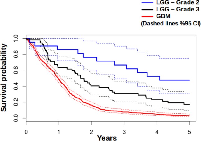
Survival probabilities for GBM (Grade IV), LGG – Grade II, and LGG – Grade II calculated from data from TCGA database

A workflow for analysis of quantitative nuclear features in glioblastoma (GBM) was previously described,^10,11 wherein individual nuclei are segmented, and then nuclear features are computed to characterize the segmented nuclei. Each individual nucleus is described using features from four categories which are nuclear morphometry, region texture, intensity, and gradient statistic. Those features are then used to assign a score to each nucleus, and a correlative analysis of the morphological score with treatment response and patient survival is carried out. When the computerized analysis results were compared to a panel of neuropathologists, the computerized analysis provided better discrimination between GBMs with differing degrees of an oligo-component, at least with regard to predicting response to therapy. This suggests that nuclear morphology analysis is a promising approach to facilitating a better understanding and diagnosis of glioma and predicting response to therapy and survival¹¹.

Deep learning has various closely related definitions or high-level descriptions, one of which is: “A class of machine learning techniques, where many layers of information processing stages in hierarchical supervised architectures are exploited for unsupervised feature learning and for pattern analysis/classification.” ¹³ The essence of deep learning is to compute hierarchical features or representations of the observational data, where the higher-level features or factors are defined from lower-level ones. The family of deep learning methods have been growing increasingly richer, encompassing those of neural networks, hierarchical probabilistic models, and a variety of unsupervised and supervised feature learning algorithms¹³.

Convolutional Neural Networks (CNNs or ConvNets), are a type of discriminative deep architecture in which layers consisting of a convolutional layer and a pooling layer are often stacked up with one on top of another to form a deep model¹⁴. The convolutional layer shares many weights, and the pooling layer subsamples the output of the convolutional layer and reduces the data rate from the layer below. The weight sharing in the convolutional layer, together with appropriately chosen pooling schemes, endows the CNN with some “invariance” properties (e.g., translation invariance). CNNs have been found highly effective and been commonly used in computer vision and image recognition ¹³. CNNs have the advantage of automatically learning the appropriate features, as opposed to traditional machine learning approaches that use hand-crafted features.

In this work, we study not only GBM (Grade IV), but also LGG (Grade II and Grade III), and we create a classification pipeline to grade histopathological images of glioma. Our work is significant in that this is a basic, yet very strong sub-typing that is strongly associated with patient survival. Our approach does not analyze single nuclei individually with classical hand-crafted machine learning features, but instead it analyzes the nuclei within the image tiles using deep learning and automatically learns the appropriate features. Best to our knowledge, deep learning has not yet been applied to pathology image analysis for glioma.

Materials and Methods

Dataset

We obtained publicly available digital diagnostic whole-slide hematoxylin and eosin (H&E) stained histopathology images (WSI) from The Cancer Genome Atlas (TCGA), which included two types of brain cancer: glioblastoma multiforme (GBM) and lower grade glioma (LGG). The LGG dataset contains Grade II and Grade III tumors.

Preprocessing

Each WSI included in the TCGA dataset can exceed 2GB in size¹¹. In order to process these images and resulting data structures, we partitioned these images into tiles. Tiling was also useful to enable parallel processing of the image to further accelerate the preprocessing.

The tile size was 1024×1024 pixels in size at the 20× resolution which is the same size and resolution used for tissue microarrays (TMAs), which can be used by a trained pathologist to make informed opinions about a whole tumor. Tiling the entire slide produces some tiles that contain little or no tissue, and only tiles that contained tissue occupying at least 90% of the tile area were chosen for further analysis¹². Tissue is distinguished by hysteresis thresholding on the grayscale and 8-bit depth complemented image, and nuclei are segmented using morphological top-hat filtering and hysteresis thresholding¹².

Due to the success of the prior nuclear morphology-based studies of GBM,^10,11 we selected to work on images in which we segment the nuclei during the preprocessing stage, but do not crop the individual nuclei, instead leave them within their original positions within the tile to not to lose the nuclei distribution map within that specific tile.

The tiles, on which we segmented the nuclei, are then further tiled to reduce in size to form samples, which we call “e-microbiopsy (electronic micro biopsy) samples,” as shown in Figure 2. This is done to reduce the sample sizes to a scale so that the deep learning networks can be trained on the GPU. Despite the attractive qualities of CNNs, and despite the relative efficiency of their local architecture, they have still been prohibitively expensive to apply in large scale to high-resolution images, and in the end, the network’s size is limited mainly by the amount of memory available on current GPUs and by the amount of training time that we are willing to tolerate²¹. For this work, we have decided for the size of the input images to the network to be 256×256 by considering the factors of GPU memory capacity, and the training time it would take for the deep learning networks.

Figure 2.

Image preprocessing (a) Whole tissue slide, (b) A single tile taken from the original image, (c) one of several electronic microbiopsy samples that are input into the deep learning pipeline, where the nuclei are segmented yet left at their original positions to preserve their inter-nuclei interaction and distributional properties.

Convolutional Neural Networks (CNNs)

CNNs are representatives of the multi-stage Hubel-Wiesel architecture, which extract local features at a high resolution and successively combine these into more complex features at lower resolutions. CNNs consist of two kinds of layers: convolutional layers (C layers), which resemble the simple cells, and pooling layers (P layers), which model the behavior of complex cells. Each convolutional layer performs a discrete 2D convolution operation on its source image with a filter kernel and applies a non-linear transfer function. The pooling layers reduce the size of the input by summarizing neurons from a small spatial neighborhood¹⁹.

The standard way to model a neuron’s output f as a function of its input x is with f(x) = tanh(x) or f(x) = (1 + e^−X)⁻¹. In terms of training time with gradient descent, these saturating nonlinearities are much slower than the non-saturating nonlinearity f(x) = max(0;x). The neurons with this nonlinearity are referred as Rectified Linear Units (ReLUs) ²⁰. Deep convolutional neural networks with ReLUs train several times faster than their equivalents with tanh units,²¹ hence we are using rectified linear units in this work.

The final layer of the CNN is fully connected to the preceding layer, which is a loss layer. The loss layer drives learning by comparing an output to a target and assigning a cost to be minimized. We use a softmax-loss as the loss layer, so the output of the fully-connected layer acts as input for the softmax classifier. The softmax loss layer computes the multinomial logistic loss of the softmax of its inputs, and it is conceptually identical to a softmax layer followed by a multinomial logistic loss layer, but provides a more numerically stable gradient²².

Implementing and Training the CNNs

The CNNs are trained with the back-propagation algorithm¹⁴. We are using Caffe²² for implementing and training the CNNs. Caffe trains models by the standard stochastic gradient descent algorithm. The CNNs are discriminatively trained via back-propagation through layers of convolutional filters and other operations such as rectification and pooling. Layers have two key responsibilities for the operation of the network as a whole: a forward pass that takes the inputs and produces the outputs, and a backward pass that takes the gradient with respect to the output, and computes the gradients with respect to the parameters and to the inputs, which are, in turn, back-propagated to earlier layers²³.

Evaluation

We tested our pipeline on independent set of data from TCGA patients who were held out during development of our method and that were not used during training and validation (our CNNs did not previously see any portion of tissue samples from these patients).

Results

Modular Deep Learning Classification Pipeline

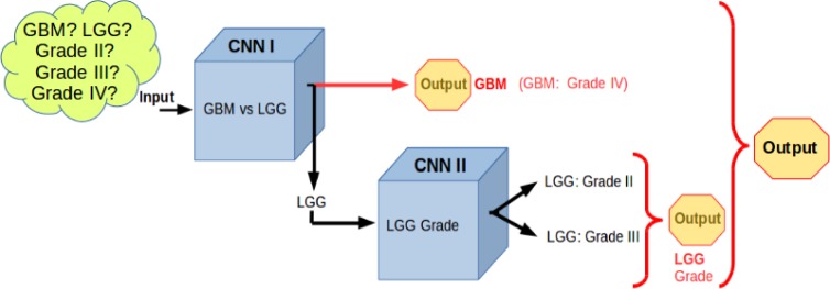
We built a modular deep learning pipeline comprising an ensemble of Convolutional Neural Networks (CNN). We created an ensemble of two CNNs, as shown in Figure 3. The first CNN classifies a histological slide to GBM vs LG, and the second CNN determines the tumor grade (grade II, grade III) for the LGG cases. By definition, GBM is a grade IV glial tumor, hence the output of pipeline yields possible grade of Grade II, Grade III or Grade IV.

Figure 3.

Modular deep learning pipeline for grading glioma using an ensemble of Convolutional Neural Networks.

Figure 4 (left) shows the structure of the first CNN that is used for GBM vs LGG classification. This CNN has a LeNeT-like architecture¹⁴ and consists of 8 layers, comprising convolution, pooling, rectified linear unit (ReLU), a fully connected (FC) layer, and finally a softmax layer. The second CNN that is used for LGG grade classification is shown on the Figure 4 (right). This network consists of 19 layers, and it is deeper compared to first CNN, but the deeper layers have a fewer number of kernels. The largest bottleneck to be aware of when selecting a CNN architecture is the available graphics processing unit (GPU) memory.

Figure 4.

(Left)The structure of the first CNN that is used for GBM vs LGG classification, (Right)The structure of the second CNN that is used for determination of LGG grade classification

At the moment, it is still difficult to design a theoretically optimal CNN architecture for a particular image classification task²⁴. Hence, a common practice is evaluating several CNNs with different layer architectures (independently to the later evaluations) in order to find a suitable CNN architecture for that particular classification task.²⁵

We trained the each individual CNN separately. When it comes to deep learning, since it could easily take several days or even weeks to train a network and there are at least thousands, sometimes millions, of data samples, it is not practical to use methods like leave-one-out cross-validation. A common practice is to have 80%–2% or 7%–3%, sometimes even 5%–50%, split of data ²¹ into training and validation sets, and use the training set to tram the network and then validation set for validation and parameter optimization purposes.

For training the first CNN we used a total of 875 e-microbiopsy samples coming from 22 whole tissue slides coming from 4 different tissue source sites, with a training subset of 6998 and validation subset of 1752 samples (80%–20% split). For training the second CNN module we used a total of 766 e-microbiopsy samples coming from 22 whole tissue slides coming from 3 different tissue source sites, with a training subset of 5671 and validation subset of 1395 samples. We stop the parameter optimization and training process once we reach a point where training error is less than or equal to 2%, and validation error is less than or equal to 1%. The factors that are taken into account for choosing these numbers include implementing early-stopping, as it is known to combat overfitting and acts as a regularization technique. Figure 5 shows the accuracy plot during the training and validation of this first CNN module for the task of GBM vs L classification.

Figure 5.

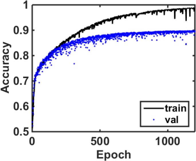
The accuracy curve for training and validation of the first CNN module that is used for GBM vs LGG classification

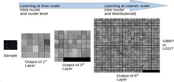
Figure 6 shows the outputs of 1^st, 3^rd and 5^th layers of the first CNN module, illustrating how the scale of information extracted changes in different layers of the network. The first layers extract features at a low-level scale, (such as intra-nuclei or single-nuclei level features); as the sample progresses through deeper layers of the network, coarser features are extracted, such as inter-nuclei and distributional properties.

Figure 6.

Visualizing an e-microbiopsy sample at different layers of processing in the first CNN: The outputs of 1st, 3rd and 5th layers are shown. Image features that are extracted vary in terms of spatial scale within different layers of the CNN.

Figure 7 shows the training and validation accuracies for the second module for the task of determining the grade of an LGG case.

Figure 7.

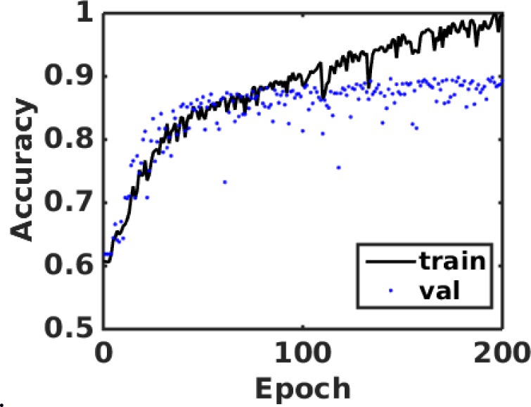
The accuracy curve for training and validation of the second CNN module that is used for grade classification of an LGG sample

Figure 8 shows the weights learned by the first layer kernels of second CNN module. This shows that the CNN has learned low-level morphological features, such as edge and arc like structures, as well as colors belonging to the nuclear stains and their opposing colors on the color wheel. Some of these features could recognize the nuclei and parts of nuclei, and some of them could recognize the inter-nuclear space, or the inter-nuclear boundaries.

Figure 8.

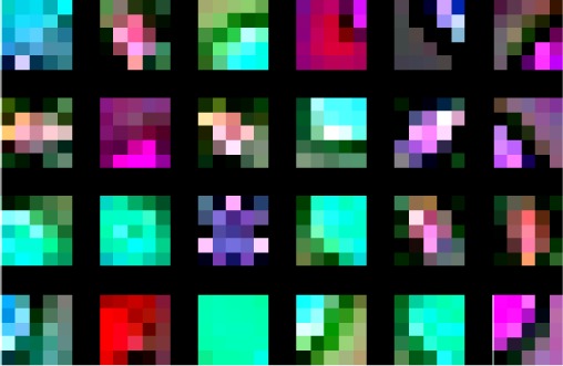
The weights learned by first twenty four of the first layer kernels of the second CNN module

Figure 9 shows the visualization of the second CNN module when an e-microbiopsy sample is fed into the network. Outputs of the first, fourth seventh and tenth layers are shown. Low level features are more local, and deeper layers reveal coarser image features through the network’s hierarchy in which higher-level features are learned from lower level features.

Figure 9.

Visualizing an e-microbiopsy sample input to the second CNN: The outputs of 1^st, 4^th, 7^th and 10^th layers are shown.

Testing on Independent Data

In our evaluation of the first CNN module, in which 10 e-microbiopsy samples were randomly selected from 10 independent test slides that had not been used during training and validation of our models, we obtained a classification accuracy of 96% for the task of GBM vs LGG classification. For the second CNN module, wherein we randomly selected 10 e-microbiopsy samples from 7 independent LGG test slides not used previously, we obtained classification accuracy of 71% for the task of Grade II vs Grade III classification for LGG. Figure 10 shows the confusion matrices and individual diagnostic qualities of these two modules and their respective tasks.

Figure 10.

Confusion matrices and diagnostic qualities of the modules

Discussion

In this work, we developed and applied a deep learning approach to the problem of automated classification of LGG vs. GBM and determination of tumor grade. We did this through the assembly of two modular CNN components, each specialized to the two different classification tasks. Our preliminary results appear to be promising, showing 96% accuracy for distinguishing LGG and GBM and 71% accuracy for distinguishing Grade II and Grade III LGG.

The task of classifying the type and grade of glioma using image features is not unlike other types of automated image feature machine learning problems in which a set of pre-defined features is used to characterize the image and predict the classification label, and our current work could have been approached using pre-defined features, such as nuclear shape, texture, etc. However, a substantial disadvantage of pre-defined features is the need to know those which are most informative in the classification task. Often the best features are not known, and a method of unsupervised feature learning could be advantageous, particularly if abundant data are available.

By not segmenting the individual nuclei into individual images as it was done in previous studies^10,11 but keeping the locality and distributional properties of them through the tissue image, our deep learning networks are extracting not only intra-nuclei and single nuclei features, but also inter-nuclei features, such as their density, distribution and interactions. Deep learning methods “let the data speak,” and they discover the relevant features in the data itself, rather than imposing pre-defined features. It could take a long time to train a CNN; however, once CNNs are trained, it is very fast to perform the classification. This is a benefit of using CNNs, as the conventional machine learning approaches with hundreds of pre-defined features could take a much longer time to classify images, compared to a CNN. Also, if the already trained networks are wanted to be updated for some reason, such as accumulation of new data that is to be included for training, the methods of transfer learning and fine tuning would enable the faster updating of the already trained networks without the need of starting a new training session from scratch which would take longer time.

We proposed and explored using an ensemble of Convolutional Neural Networks to form a modular decision pipeline. There are various reasons that we chose to have an ensemble of modular and rather simpler CNNs, as opposed to using a single, but more complex monolithic CNN. First, we would like to be able to gauge measures of the diagnostic quality and statistical measures of the performance of the test, when it comes to decision making in biomedical field. Having such a modular structure enables us to analyze the diagnostic quality of each individual decision step. Second, we opted for having a pipeline with modular units at each decision step, as this would make it easier to analyze each smaller unit independently and help to obtain features that are more intuitive or interpretable, compared to having a single yet very complex unit which could make it difficult to gain intuition regarding its operation. Third, the size of image datasets are generally smaller in the medical domain due to challenges of acquiring many images, and CNNs are difficult to train using small datasets. ¹⁵ Hence, in this work, we opted for training smaller networks with fewer output classes compared to a single, very deep and complex one, with the outputs representing all possible cases in which we are interested. As the number of output classes increases, the more samples might be needed to train a network well. Fourth, by having modular CNN units, we could explore different network architectures. For example, in our case, in one unit we had a shallower network with higher number of kernels per layer, and another network was deeper with fewer number of kernels per layer. Finally, having such a modular structure could enable users to be able to selectively use specific paths or units along the pipeline. Such modularity would allow us to integrate our single units to probabilistic graphical models, such as Bayesian networks and Markov decision processes, or to combine with other machine learning approaches such as Support Vector Machines (SVM).

The results of our evaluation of accuracy for LGG Grade classification on independent data (71%) is a reasonable preliminary result, but leaves room for improvement. There are several potential reasons for this performance. First, TCGA data vary in terms of coming from multiple centers, each of which processes the tissues with non-uniform protocols for tissue slicing, staining, image acquisition, and timing of the steps. Differences in slide preparation, microscope, and digitizing device between two batches of data may lead to differences in image properties between the two batches, and these differences, called “batch effects,” can bias the performance estimates of predictive models.¹⁶ The quality of WSI is also affected by artifacts introduced during image acquisition and batch effects, resulting from variations in experimental protocol. Data quality is especially challenging in collaborative repositories, such as TCGA, where a large amount of high-throughput data is collected from multiple institutions.¹⁶ Apart from artifacts introduced during tissue processing and image acquisition, there are variations within the tissue slides, and portions of pathology images could contain non tumor tissue which may or may not be relevant to the diagnosis, so classification accuracy can be further improved by considering a set of e-microbiopsy samples from a slide and making the decision via a majority voting like scheme. Future work in which our methods are applied to more homogenous data (e.g., that from a single instruction) would be interesting to establish the magnitude of these confounding aspects on the accuracy of our results. Such future work could also motivate research efforts to reduce the impact of such variations on methods such as ours.

Another factor that could impair the accuracy of our method in classifying LGG grade is that the distinction between a Grade II vs Grade III glioma is more subtle compared to distinguishing Grade IV from Grades II and Grade III. It has been noted that significant problems relate to the interpretation of histologic criteria used to classify and grade gliomas.^17,18 Problems with tumor grading are most significant for intermediate grade tumors, for which patient survival broadly overlaps that associated with lower and higher grade tumors.⁹ Our results also agree with these prior observations.

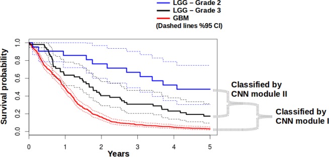
In terms of survival, if we look at the plot calculated from the survival data of all samples in TCGA (Figure 11), GBM cases are clearly distinct, with a very low probability of survival. For LGG Grade II and LGG Grade III, even though the main rate curves are separated, the %95 confidence intervals are overlapping. So, from the survival point of view, the accuracies of CNN modules also share similar behavior, similar to previous observations from others that there are challenges in tumor grading in intermediate grade tumors, for which patient survival broadly overlaps.⁹ On the other hand, our modular pipeline has advantages, because each unit can be executed individually (i.e., classifying GBM vs LGG). Though pathologists can likely distinguish LG and GBM with similar accuracy as our approach, our methods could be useful in quality improvement initiatives, as a “second look,” or teaching applications. Our modular approach lets us meet the requirements of minimum accuracy levels that are demanded by the context of different decision points within a multi-class (i.e. more than 2 classes) classification scheme.

Figure 11.

Survival probabilities for GBM (Grade IV), LGG Grade II, and LGG Grade III, shown alongside the respective CNN modules that perform the classification

Moreover, to our knowledge, our work is the first to apply deep learning methods to the task of pathology image diagnosis and classification of tumor grade. There are many facets of CNN architectural optimization that we have not yet explored which we plan on pursuing in future work. We will also work on ways to improve our accuracy by exploring extra steps during the preprocessing stage, and also including information from the tissue stroma.

Conclusion

We developed a deep learning-based modular pipeline with ensemble of CNNs for the problem of classification and grading of glioma from digital pathology images. Our modular classification pipeline approach has the advantages of having diagnostic quality statistics of individual modules, making it easier to train these models given limited data availability and being able to explore different CNN structures for each module, facilitating relatively smaller hence easier to analyze CNNs, and giving flexibility to be used as single modules or within the framework of other modeling or machine learning applications. Our deep learning based classification modules achieved more than 90% accuracies on validation data set, and our approach produced 96% accuracy for GBM vs LGG classification, and 71% accuracy for LGG Grade I vs LGG Grade II discrimination on an independent data set coming from new patients from a collaborative repository where data is collected from multiple institutions. These results may be improved in future by leveraging our modular approach enabling us to address and optimize the different components of the task (diagnosis of GBM vs LGG, and determination of tumor grade) separately.

References

- 1.Ostrom QT, et al. The epidemiology of glioma in adults: a “state of the science” review. Neuro Oncol. 2014;16(7):896–913. doi: 10.1093/neuonc/nou087. [DOI] [PMC free article] [PubMed] [Google Scholar]
- 2.Ostrom QT, et al. CBTRUS statistical report: primary brain and central nervous system tumors diagnosed in the United States in 2006–2010. Neuro-oncol. 2013;15:iil–56. doi: 10.1093/neuonc/not151. sup 6. [DOI] [PMC free article] [PubMed] [Google Scholar]
- 3.Louis DN, et al. The 2007 WHO classification of tumours of the central nervous system. Acta Neuropathol. 2007;114(2):97–109. doi: 10.1007/s00401-007-0243-4. [DOI] [PMC free article] [PubMed] [Google Scholar]
- 4.Kettenmann H, Ransom R, Neuroglia BR. Oxford University Press; 2012. [Google Scholar]
- 5.Sant M, Minicozzi P, Lagorio S, et al. Survival of European patients with central nervous system tumors. Int J Cancer. 2012;131(1):173–185. doi: 10.1002/ijc.26335. [DOI] [PubMed] [Google Scholar]
- 6.Crocetti E, Trama A, Stiller C, et al. Epidemiology of glial and non-glial brain tumours in Europe. Eur J Cancer. 2012;48(10):1532–1542. doi: 10.1016/j.ejca.2011.12.013. [DOI] [PubMed] [Google Scholar]
- 7.Tseng MY, Tseng JH, Merchant E. Comparison of effects of socioeconomic and geographic variations on survival for adults and children with glioma. J Neurosurg. 2006;105(Suppl 4):297–305. doi: 10.3171/ped.2006.105.4.297. [DOI] [PubMed] [Google Scholar]
- 8.Jung KW, Yoo H, Kong HJ, et al. Population-based survival data for brain tumors in Korea. J Neurooncol. 2012;109(2):301–307. doi: 10.1007/s11060-012-0893-5. [DOI] [PubMed] [Google Scholar]
- 9.Coons SW, Johnson PC, Scheithauer BW, Yates AJ, Pearl DK. Improving diagnostic accuracy and interobserver concordance in the classification and grading of primary gliomas. Cancer. 1997;79:1381–1393. doi: 10.1002/(sici)1097-0142(19970401)79:7<1381::aid-cncr16>3.0.co;2-w. [DOI] [PubMed] [Google Scholar]
- 10.Kong J, et al. Machine-based morphologic analysis of glioblastoma using whole-slide pathology images uncovers clinically relevant molecular correlates. PLoS One. 2013 Nov 13;8(11):e81049. doi: 10.1371/journal.pone.0081049. [DOI] [PMC free article] [PubMed] [Google Scholar]
- 11.Kong J, et al. In silico analysis of nuclei in glioblastoma using large-scale microscopy images improves prediction of treatment response. Conf Proc IEEE Eng Med Biol Soc. 2011 Aug;2011:87–90. doi: 10.1109/IEMBS.2011.6089903. [DOI] [PMC free article] [PubMed] [Google Scholar]
- 12.Barker J et al., Automated classification of brain tumor type in digital pathology images using local representative patches (submitted).
- 13.Deng L, Yu D. Deep Learning: Methods and applications foundations and trends in signal processing. 2014. Now Publishers Incorporated. [Google Scholar]
- 14.LeCun Y, Bottou L, Bengio Y, Haffner P. Gradient-based learning applied to document recognition. Proceedings of the IEEE. 1998;86:2278–2324. [Google Scholar]
- 15.Oquab M, et al. CVPR ‘14 Proceedings of the 2014 IEEE Conference on Computer Vision and Pattern Recognition Pages; pp. 1717–1724. [Google Scholar]
- 16.Kothari S, et al. Pathology imaging informatics for quantitative analysis of whole-slide images. J Am Med Inform Assoc. 2013;20:1099–1108. doi: 10.1136/amiajnl-2012-001540. [DOI] [PMC free article] [PubMed] [Google Scholar]
- 17.Daumas-Duport C, Scheithauer B, O’Fallon J, Kelly P. Grading of astrocytomas: a simple and reproducible method. Cancer. 1988;62:2152–65. doi: 10.1002/1097-0142(19881115)62:10<2152::aid-cncr2820621015>3.0.co;2-t. [DOI] [PubMed] [Google Scholar]
- 18.Weller RO. Grading of brain tumours: the British experience. Neurosurg Rev. 1992;15:7–11. doi: 10.1007/BF02352059. [DOI] [PubMed] [Google Scholar]
- 19.Scherer D, Miiller A, Behnke S. Evaluation of pooling operations in convolutional architectures for object recognition; Artificial Neural Networks-ICANN; 2010. pp. 92–101. [Google Scholar]
- 20.Nair V, Hinton GE. Rectified linear units improve restricted boltzmann machines; Proc. 27th International Conference on Machine Learning; 2010. [Google Scholar]
- 21.Krizhevsky A, Sutskever I, Hinton GE. Imagenet classification with deep convolutional neural networks. Advances in neural information processing systems. :1097–1105. [Google Scholar]
- 22.Caffe: Deep learning framework by the Berkeley Vision and Learning Center. http://caffe.berkeleyvision.org/
- 23.Yangqing J, et al. Caffe: Convolutional Architecture for Fast Feature Embedding; Proceedings of the ACM International Conference on Multimedia; New York, NY, USA: ACM; 2014. pp. 675–678. [Google Scholar]
- 24.Zeiler MD, Fergus R. Visualizing and understanding convolutional networks. Computer Vision–ECCV. 2014:818–833. [Google Scholar]
- 25.Roth HR, et al. Detection of Sclerotic Spine Metastases via Random Aggregation of Deep Convolutional Neural Network Classifications, Recent Advances in Computational Methods and Clinical Applications for Spine Imaging. Lecture Notes in Computational Vision and Biomechanics. 2015;20:3–12. [Google Scholar]