MeSHLabeler: improving the accuracy of large-scale MeSH indexing by integrating diverse evidence

Abstract

Motivation: Medical Subject Headings (MeSHs) are used by National Library of Medicine (NLM) to index almost all citations in MEDLINE, which greatly facilitates the applications of biomedical information retrieval and text mining. To reduce the time and financial cost of manual annotation, NLM has developed a software package, Medical Text Indexer (MTI), for assisting MeSH annotation, which uses k-nearest neighbors (KNN), pattern matching and indexing rules. Other types of information, such as prediction by MeSH classifiers (trained separately), can also be used for automatic MeSH annotation. However, existing methods cannot effectively integrate multiple evidence for MeSH annotation.

Methods: We propose a novel framework, MeSHLabeler, to integrate multiple evidence for accurate MeSH annotation by using ‘learning to rank’. Evidence includes numerous predictions from MeSH classifiers, KNN, pattern matching, MTI and the correlation between different MeSH terms, etc. Each MeSH classifier is trained independently, and thus prediction scores from different classifiers are incomparable. To address this issue, we have developed an effective score normalization procedure to improve the prediction accuracy.

Results: MeSHLabeler won the first place in Task 2A of 2014 BioASQ challenge, achieving the Micro F-measure of 0.6248 for 9,040 citations provided by the BioASQ challenge. Note that this accuracy is around 9.15% higher than 0.5724, obtained by MTI.

Availability and implementation: The software is available upon request.

Contact: zhusf@fudan.edu.cn

1 Introduction

As a controlled vocabulary, Medical Subject Headings (MeSH) (http://www.nlm.nih.gov/mesh/meshhome.html) is developed by National Library of Medicine (NLM) for indexing almost all citations in the largest biomedical literature database, MEDLINE (http://www.nlm.nih.gov/pubs/factsheets/medline.html), which currently covers more than 5600 journals world-wide (NCBI Resource Coordinators, 2015; Nelson et al., 2004). The documents, books and audiovisuals recorded in NLM are also cataloged by MeSH. MeSH is organized hierarchically and updated annually with minor changes. By 2014, there are 27,149 MeSH main headings (MHs) (http://www.nlm.nih.gov/pubs/factsheets/mesh.html). On average each citation in MEDLINE is annotated by 13 MHs to describe its content. In addition to indexing, MeSH has been widely used to facilitate many other tasks in biomedical information retrieval and text mining, such as query expansion (Lu et al., 2010; Stokes et al., 2010) and document clustering (Gu et al., 2013; Huang et al., 2011b; Zhu et al., 2009a, b). Accurate MeSH annotation is thus very important for biomedical researchers for knowledge discovery.

Currently indexing MEDLINE is mainly performed by a number of highly qualified NLM staff and contractors, who review the full text of each article and assign suitable MeSH headings. It is estimated that the average cost of annotating an article is around $9.4 (Mork et al., 2013). In the last few years, the number of citations indexed in MEDLINE has been dramatically increased, reaching more than 21 million. In 2014, 765,850 citations have been indexed, which is around 4% increase over 2013 (734,052) (http://www.nlm.nih.gov/bsd/bsd_key.html). The high growth of MEDLINE poses a great challenge to the NLM indexers to finish the MeSH indexing task effectively and efficiently. A software tool, Medical Text Indexer (MTI), has been developed in NLM to support the indexers with MeSH recommendations (Aronson et al., 2004; Mork et al., 2013, 2014). MTI uses only the titles and abstracts of documents in MEDLINE as input, and outputs MeSH as recommendation. There are two most important components in MTI, MetaMap Indexing (MMI) and PubMed-Related Citations (PRC). MMI uses MetaMap, a software tool for mapping the text to biomedical concepts (Aronson and Lang, 2004), to find concepts appearing in the titles and abstracts, which are then used to specify MHs. PRC first finds neighbors (similar citations) in MEDLINE by using PubMed-related articles (PRA) (Lin and Wilbur, 2007), a modified k-nearest neighbor (KNN) algorithm, and then extracts their MHs. These two sets of MHs are linearly combined and turned into an ordered list of MHs. Finally, after several steps of post-processing, like expanding CheckTags (some special MHs), a final list of MHs is suggested to MeSH indexers.

Many studies have addressed the challenging problem of automatic MeSH indexing. In this problem, each MH can be regarded as a class label and each citation can have multiple MHs, and so the MeSH indexing is a large-scale multi-label classification problem (Zhang and Zhou, 2014). The difficulty of this problem can be attributed to the following three factors: (i) The number of distinct MHs is large and their distribution is biased. Table 1 shows six MeSH, ranked as first, 100th, 1000th, 10,000th, 20,000th and 25,000th in terms of their frequencies in the all 12,504,999 MEDLINE citations with abstracts. The most frequent MH, Humans, appears in 8,152,852 citations, while the 25,000th frequent MH, Pandanaceae, appears in 31 citations only. This means that most of all 27,149 MeSH have very few positively annotated citations, resulting in a serious imbalance between the number of positives and negatives; (ii) There are large variations in the number of MeSH for each citation. One citation may have 30 MHs, while another may have only five MHs; (iii) Usually full text is unavailable for automatic MeSH indexing, and important MeSH concepts might exist in the full text only.

Table 1.

The first, 100th, 1000th, 10,000th, 20,000th and 25,000th MeSH in terms of the number of appearances in 12,504,999 abstracts, which we used in our experiments

Rank	Counts	MeSH (ID)
1	8,152,852	Humans (6801)
100	129,816	Risk Assessment (18,570)
1000	23,178	Soil (12,987)
10,000	1532	Transplantation Tolerance (23,001)
20,000	199	Hypnosis, Anesthetic (6991)
25,000	31	Pandanaceae (31,673)

To advance the design of effective algorithms for biomedical semantic indexing and question answering, BioASQ challenge, a European project, established an international competition in 2013 and 2014 with two tasks: (A) automatically annotating new MEDLINE citations using MeSH and (B) answering questions set by the European biomedical expert team of BioASQ (http://bioasq.org) (Balikas et al., 2014; Partalas et al., 2013). Task A of 2014 BioASQ challenge consists of three rounds, with each round having 5 weeks. In each week, 3496–8840 new MEDLINE citations (titles and abstracts) are provided to the challenge participants, and prediction results must be submitted within 21 h. Our system won the first place in the second and third rounds of this task (Balikas et al., 2014). In thisarticle, we present MeSHLabeler, the underlying algorithm of our system in detail, with thorough experiment and comprehensive analysis of the experimental results.

MeSHLabeler integrates different types of evidence in the framework of ‘learning to rank’ (Liu, 2011) for accurate MeSH annotation in the following manner: First, for each citation, the system generates a list of candidate MHs, and then each candidate is represented by a number of features. Two models, named as MeSHRanker and MeSHNumber, for predicting (ranking) MHs of an arbitrary citation and predicting the number of MHs of the citation, respectively, are then trained by using a set of citations. MeSHRanker provides prediction scores for the candidate MHs to rank them, and finally the top of the ranked MHs are obtained as prediction results by MeSHNumber. The most challenging problem in MeSH indexing is the imbalance between positives and negatives. MeSHLabeler solves this by using a sufficiently large set of features (evidence), classified into mainly five types: global evidence, local evidence, MeSH dependency, pattern matching and MTI: (i) The global evidence comes from MeSH classifiers, which are trained by using the entire MEDLINE collection. Each classifier is trained independently, and thus prediction scores from different classifiers are not comparable. MeSHLabeler has an original score normalization method that can address this issue and improve the performance significantly. (ii) The local evidence is given by scores from the most similar citations (nearest neighbors). (iii) MeSH dependency, which is a unique feature of MeSHLabeler, explicitly considers the MeSH–MeSH pair correlations in an efficient way. It improves the indexing performance, particularly for predicting infrequent MHs. Due to the high computational burden caused by the huge number of MeSH–MeSH combinations, all previous studies have not considered the MeSH dependency. (iv) Pattern matching directly finds MHs or their synonyms in the titles and/or abstracts using string matching. (v) MTI considers not only pattern matching and local evidence, but also indexing rules with domain knowledge, like ‘An article with subjects ranging from 25 to 44 in age would have the check tag, ADULT, only’. This type of indexing rules is useful, so we incorporate the results of MTI into MeSHLabeler.

The performance advantage of MeSHLabeler was demonstrated in the 2014 BioASQ challenge. In this article, we further examined the performance of MeSHLabeler more thoroughly using 12,504,999 citations downloaded from MEDLINE and 51,724 citations from 2014 BioASQ challenge. From the series of experiments, MeSHLabeler achieved the Micro F-measure of 0.6248, which was around 9.15% higher than that of 0.5724 by MTI.

2 Related work

A number of studies have addressed the problem of indexing large-scale biomedical documents by using different types of data and models (Jimeno-Yepes et al., 2012a). Researchers in NLM have also examined not only MTI but also other methods by using different machine learning algorithms, such as naive Bayes classifiers, support vector machines (SVMs) and AdaBoostM1 over a medium-sized dataset with around 300,000 citations (Jimeno-Yepes et al., 2012b, 2013a). They found that no single algorithm could perform the best and a combination of various algorithms, such as simple voting, could improve the performance of MTI. They also explored the effect of using full text and summary, which results in better recall but lower precision than using only abstracts (Jimeno-Yepes et al., 2013b). In addition, Ruch (2006) proposed a method by combining information retrieval and pattern matching for MeSH indexing. Trieschnigg et al. (2009) found that KNN outperformed thesaurus-oriented and concept-oriented classifiers. A serious concern on this study is that their training and evaluation datasets were relatively small.

The BioASQ challenge provides a benchmark for comparing the performance of different algorithms on large-scale MeSH indexing. The best system in the 2013 BioASQ challenge used the algorithm of MetaLabeler (Tang et al., 2009) and outperformed MTI slightly (Tsoumakas et al., 2013). The developers of this system examined many multi-label classification algorithms and found that a simple yet effective algorithm, MetaLabeler, performed the best. They trained linear SVM as a binary classifier for each MeSH, and trained a regression model for predicting the number of MHs of each citation. In prediction, for a given citation, candidate MHs are ranked, according to the prediction scores of each MH classifier, and then top K MHs are returned as recommendation, where K is the predicted number of MHs. One big problem of this method is that the prediction scores of different MH classifiers cannot be compared directly in principle, causing low quality of ranking MHs. For this problem, the second best system in 2013 BioASQ challenge used ‘learning to rank’ (Huang et al., 2011a; Mao and Lu, 2013), while the features of this system were from KNN, MTI and information retrieval mainly. Note that it did not use global evidence (classifier predictions), which must be important for MeSH indexing. This system was improved for the 2014 BioASQ challenge by incorporating multiple binary classifier results, while they are not directly comparable in principle (Mao et al., 2014). In addition, a heuristic was used for predicting the number of final MHs.

Overall no existing approach has simultaneously addressed the following two important issues: (i) comparing the prediction scores of different MHs classifiers; and (ii) incorporating the dependency of different MHs. MeSHLabeler addresses these two crucial issues efficiently and effectively and it outperforms the state-of-the-art approach, MTI, by nearly 10% improvement in micro F-measure.

3 Methods: MeSHLabeler

3.1 Overview: MeSHLabeler = MeSHRanker + MeSHNumber

The problem setting is as follows: given an arbitrary MEDLINE citation with title and abstract, we assign a certain number of MHs out of all possible MHs (>27,000). Figure 1a shows the work flow of MeSHLabeler, which has two components: MeSHRanker and MeSHNumber. For each input citation, MeSHRanker returns an ordered list of candidate MHs and MeSHNumber predicts the number of MHs as the output from the candidate list.

Fig. 1.

The work flow of (a) MeSHLabeler and (b) MeSHRanker

3.2 Preliminaries

Our problem is multi-label classification. It can be solved using MetaLabeler, a simple method that we will use as a baseline. Before going to MetaLabeler, we need to review a binary classification problem, in which each MH is a binary class and each citation is one instance. Logistic regression (LogReg) and KNN, are two well-accepted classification methods, which will be used in MetaLabeler and MeSHLabeler. Note that these two approaches are complementary from a machine learning perspective: LogReg uses the entire database to train the model, attempting to capture global evidence, while KNN focuses on similar instances, attempting to capture local evidence. We start with the description of these two approaches and then MetaLabeler.

3.2.1 Logistic regression

We use a general optimization method for estimating parameters of LogReg. We use the entire set of MEDLINE records (see Section 4.1 for detail) to train parameters of LogReg to capture global evidence.

3.2.2 k-nearest neighbor

For KNN, we need similar citations and their similarity scores. For this purpose, we use NCBI efetch (http://www.ncbi.nlm.nih.gov/books/NBK25499/) to retrieve similar citations by PRA (Lin and Wilbur, 2007), which is analogous to the KNN algorithm. The MHs in the retrieved citations can be promising candidates for annotating MHs. Thus given a target citation, we compute the score of candidate MH as follows:

$$\frac{{\displaystyle {\sum }_{i=1}^{K_{\text{NN}}}(S_i·B_i)}}{{\displaystyle {\sum }_{i=1}^{K_{\text{NN}}}{S}_i}},$$ (1)

where K_NN is the number of most similar citations, S_i is the similarity score of the ith citation and B_i is a binary variable to indicate if the candidate MH is annotated in the ith citation or not.

3.2.3 MetaLabeler

It is a straight-forward but powerful approach for solving the problem of multi-label classification (Tang et al., 2009), which is based on two different types of classifiers.

• 1. Classifier A

• We train a binary classifier (the default is SVM but replaceable) for each label (MH in our problem), and repeat this training over all labels independently. Given an instance (citation in our problem), we run all trained classifiers to obtain prediction scores of all labels and rank all labels, according to the prediction scores.

• 2. Classifier B

• We train a classifier to predict the number of labels for each instance. Given an instance, the number of labels is predicted by this classifier.

• 3. Final prediction

• Given an instance, we select a certain number of top labels from the ranked list obtained by Classifier A, by using the number (of labels) predicted by Classifier B.

Note again that any binary classifier can be used in Classifier A, and LogReg is a good option in terms of efficiency. Hereafter, we call MetaLabeler as MLogReg if LogReg is used for Classifier A, and we further call MLogRegN if score normalization (to be described later) is used for comparing multiple MHs in MLogReg.

The main flow of MetaLabeler is incorporated into MeSHLabeler, and so MetaLabeler can be a baseline to be compared in performance with MeSHRanker. Furthermore, MeSHLabeler has many other important features, such as prediction score normalization over multiple labels, dependency between labels and learning to rank. They will significantly improve the predictive performance of the baseline method, MetaLabeler.

3.3 MeSHRanker

Figure 1b shows the procedure of MeSHRanker. We will explain MeSHRanker accordingly.

3.3.1 Step 1: generate candidate MeSH

We have a very large number of classes (labels), i.e. more than 27,000 MeSH, for a multi-label classification problem. To reduce irrelevant MHs as well as extra computational burden in the following steps, we first focus on a limited number of MHs by generating candidate MHs for each target citation in the following manner: we obtain a list, L_LogReg, of MHs predicted (and ranked) by LogReg (global evidence), which was already trained by using the entire MEDLINE, and also list, L_KNN, by KNN (local evidence), according to Equation (1). We then merge them together to have the candidate MHs, which satisfy at least one of the following two requirements:

• appearing in the top N_Log Reg of L_Log Reg

• appearing in the top N_KNN of L_KNN

3.3.2 Step 2: generate features for ranking MHs in Step 3

We generate the following seven different types of features.

• 1. MetaLabeler with LogReg (MLogReg)

• The original MetaLabeler uses an SVM. Here, we choose LogReg, keeping the other parts totally the same as MetaLabeler. We note that MLogReg uses all citations, meaning global evidence.

• Practically, for each MH, we use one million latest citations for training, by ordering all citations from the most recent to the oldest. For infrequent MHs, we collect citations until the number of positives becomes the same as negatives or all citations are examined. This data size setting is large enough to avoid any overfitting issues.

• 2. KNN

• We use Equation (1) for KNN.

• 3. MLogReg with score normalization (MLogRegN)

• We normalize the original prediction scores by MLogReg in the following manner: Prediction scores for all citations are first ranked in the descending order. Since each citation is positive or negative, we can then compute the precision of the prediction of each citation by dividing the number of positives that are more highly ranked, by the number of all positives. This means that any score (for some citation) can be transformed into precision, which takes a range from zero to one. For each MH, the normalized score via precision represents the probability of being a true annotation, which is directly comparable. We perform this transformation for each MH, and use precisions for all MHs, as normalized scores.

• Practically, due to the limitations of available computing resources, we used one million latest citations for score normalization.

• 4. MeSH dependency

• For a candidate MH, denoted by $\widehat{\text{MH}}$, the score of MeSH dependency can be computed as follows:

  $${\displaystyle \sum _{i=1}^{K_{\text{MeSH depend}}}{f}_{\text{MLogRegN}}}({\text{MH}}_i)·P(\widehat{\text{MH}}|{\text{MH}}_i),$$ (2)
• where ${\text{MH}}_i$ is the top ith MH in the candidate list ranked by MLogRegN, $f_{\text{MLogRegN}}({\text{MH}}_i)$ is the score of ${\text{MH}}_i$ predicted by MLogRegN and $P(\widehat{\text{MH}}|{\text{MH}}_i)$ is the conditional probability of $\widehat{\text{MH}}$ given ${\text{MH}}_i$. $P(\widehat{\text{MH}}|{\text{MH}}_i)$ is obtained as follows:

  $$P(\widehat{\text{MH}}|{\text{MH}}_i)=\frac{|N(\widehat{\text{MH}},{\text{MH}}_i)|}{|N({\text{MH}}_i)|},$$

• where $N({\text{MH}}_i)$ is the number of appearances of ${\text{MH}}_i$ in the entire MEDLINE, and $N(\widehat{\text{MH}},{\text{MH}}_i)$ is the number of co-occurring appearances of $\widehat{\text{MH}}$ and ${\text{MH}}_i$ in the entire MEDLINE.

• Intuitively, this feature indicates that $\widehat{\text{MH}}$ is more likely to be a true annotation, if $\widehat{\text{MH}}$ is highly correlated with highly ranked MHs.

• 5. Pattern matching

• We can check if the content of the target citation (title and/or abstract) has each MH directly. The procedure is as follows: (i) for each MH, the entry term and synonyms can be retrieved from the MeSH thesaurus, (ii) the title and abstract of one citation are scanned, and 1 is assigned if the corresponding MeSH entry term or synonyms are found; otherwise 0. We can thus generate two binary features for the entry term and the synonyms. This is computationally light, because the target citation is checked only once by string matching without checking any other citations. Also we note that pattern matching can be conducted in the following three ways: titles only, abstracts only and both titles and abstracts.

• 6. MeSH frequency

• We can compute the probability of appearing $\widehat{\text{MH}}$ in the journal of a citation, as follows:

  $$\frac{|N(\widehat{\text{MH}})|}{N_J},$$

• where N_J is the number of all citations in journal J and $N(\widehat{\text{MH}})$ is the occurrences of $\widehat{\text{MH}}$ in all citations of journal J.

• 7. MTI

• We can use the MHs recommended by MTI, which integrates KNN, pattern matching and indexing rules, as features. We use two options of MTI: default (MTIDEF) and MTI FirstLine Index (MTIFL). MTIDEF attempts to achieve a balance between precision and recall, while MTIFL recommends a smaller number of MHs, which have high precision. We then generate two binary features.

3.3.3 Step 3: rank MeSH by learning to rank

We rank the MHs by using ‘learning to rank’, which is widely used in information retrieval for ranking documents with respect to a query according to relevance (Liu, 2011). In MeSHRanker, each citation and MHs are a query and document, respectively, meaning that candidate MeSH is ranked by the relevance to the citation that needs to be annotated. A lot of methods have been proposed for learning to rank. Here, we use Lambda MART (Burges, 2010), which has been successfully applied to a number of real-world problems. We again emphasize that our idea is to integrate multiple, independent and different evidence in the framework of ‘learning to rank’.

3.4 MeSHNumber

MeSHNumber predicts the number of MHs to be selected from the top of the output of MeSHRanker. The key point of this part is to use multiple, different and diverse features to achieve high predictability on the number of MHs for each citation. We first generate the following six different types of features, and for prediction, we use support vector regression (SVR).

• 1 Citations in the same journal

• We check the number of MHs annotated for citations which are published in the same journal and the same year as those of the target citation. We then compute the mean and standard deviation over these citations, to be used as features. Similarly, we check the numbers of MHs of five citations in the same journal whose published dates are the closest to the published date of the target citation. Their mean and standard deviation are also used as features.

• 2. PubMed-related articles

• We check the number of MHs of M_PRA most similar citations computed by PRA, and use their mean and standard deviation as features.

• 3. LogReg

• We choose the M_LogReg highest scores for predicting MHs by LogReg for the target citation and directly use these scores as features. Note that these scores can be obtained in Step 1 of MeSHRanker.

• 4. Learning to rank

• We choose the top M_LTR scores for predicting MHs by learning to rank for the target citation and directly use these scores as features. Note that these scores can be obtained in Step 3 of MeSHRanker.

• 5. MetaLabeler

• We train MetaLabeler for predicting the number of MHs (the option is SVR) and use the prediction result as a feature.

• 6. MTI

• We use the number of MHs predicted by MTIDEF and MTIFL as two features.

4 Experiments

4.1 Data

We downloaded 22,376,811 citations of MEDLINE/PubMed from NLM before the BioASQ 2014 challenge. We filtered out the citations with no abstracts and obtained 12,504,999 citations, which were stored locally as a training set. They were tokenized and stemmed by BioTokenizer (Jiang and Zhai, 2007), resulting in a dictionary of 3,712,632 tokens. As in the work (Tsoumakas et al., 2013), we used unigram and bigram features to represent each citation, and we only considered those which appear six or more times in the entire data. This is because rare unigram/bigram features are less informative and keeping them makes all computation expensive. We obtained 111,034 unigram and 1,867,013 bigram features, and each citation is represented by a very sparse vector with only 1,978,047 elements. Also we used a TF-IDF scoring scheme to assign a weight to each unigram/bigram feature. They were used for training LogReg mainly.

We then further downloaded 51,724 citations of a benchmark dataset from the BioASQ challenge, where we randomly chose 32,684 citations for training of Step 3 in MeSHRanker, 10,000 citations for training MeSHNumber and 9040 citations for examining the performance of MeSHLabeler. For 51,724 citations, on average, each citation has 10.3 sentences and 162.6 words. To make a fair comparison, the performance of all methods was examined on these 9040 citations.

4.2 Implementation

We used an open-source tool, RankLib (http://sourceforge.net/p/lemur/wiki/RankLib/), to implement Lambda MART (Burges, 2010). LogReg and SVM were implemented by using LIBLINEAR (Fan et al., 2008). SVR was implemented by using LIBSVM (Chang and Lin, 2011).

4.3 Performance evaluation measure

We use three different metrics, all based on F-measure, a measure commonly used in information retrieval. F-measure is computed using precision and recall, and so for each F-measure of the three different metrics, two further measures, i.e. precision and recall, are attached, resulting in totally nine evaluation measures.

4.3.1 Notation

Let K denote the size of all MeSH headings, and N be the number of instances. Let y_i and ${\widehat{y}}_i\in {\{0,1\}}^K$ be the true and predicted label for instance (citation) i, respectively.

4.3.2 Three types of F-measures (with precision and recall)

• • F-measure: EBF

• EBF is the standard F-measure which can be computed as the harmonic mean of standard precision (EBP) and recall (EBR), as follows:

  $$\text{EBF}=\frac{1}{N}{\displaystyle \sum _{i=1}^N}{\text{EBF}}_i,$$ (3)

  where

  $${\text{EBF}}_i=\frac{2·{\text{EBP}}_i·{\text{EBR}}_i}{{\text{EBP}}_i+{\text{EBR}}_i},$$

  where

  $${\text{EBP}}_i=\frac{{\displaystyle {\sum }_{k=1}^K{y}_i^k}·{\widehat{y}}_i^k}{{\displaystyle {\sum }_{k=1}^K·}{\widehat{y}}_i^k}{\text{EBR}}_i=\frac{{\displaystyle {\sum }_{k=1}^K{y}_i^k}{\widehat{y}}_i^k}{{\displaystyle {\sum }_{k=1}^K{y}_i^k}}.$$

  We note that we can compute EBP and EBR by summing EBP_i and EBR_i, respectively, over all instances.

• • Macro F-measure: MaF

• MaF is the harmonic mean of macro-average precision (MaP) and macro-average recall (MaR) as follows:

  $$\text{MaF}=\frac{2·\text{MaP}·\text{MaR}}{\text{MaP}+\text{MaR}}$$ (4)

The MaP and MaR are obtained by first computing the precision for each label (MH) separately and then averaging over all labels, as follows:

$$\text{MaP}=\frac{1}{K}{\displaystyle \sum _{k=1}^K{\text{P}}^k}\text{\hspace{1em}MaR}=\frac{1}{K}{\displaystyle \sum _{k=1}^K{\text{R}}^k},$$

where

$${\text{P}}^k=\frac{{\displaystyle {\sum }_{i=1}^N{y}_i^k}·{\widehat{y}}_i^k}{{\displaystyle {\sum }_{i=1}^N{\widehat{y}}_i^k}}{\text{R}}^k=\frac{{\displaystyle {\sum }_{i=1}^N{y}_i^k}·{\widehat{y}}_i^k}{{\displaystyle {\sum }_{i=1}^N{y}_i^k}}.$$

• • Micro F-measure: MiF

• MiF is the harmonic mean of micro-average precision (MiP) and micro-average recall (MiR), as follows:

  $$\text{MiF}=\frac{2·\text{MiP}·\text{MiR}}{\text{MiP}+\text{MiR}},$$ (5)

  where

  $$\text{MiP}=\frac{{\displaystyle {\sum }_{k=1}^K{\displaystyle {\sum }_{i=1}^N{y}_i^k}}·{\widehat{y}}_i^k}{{\displaystyle {\sum }_{k=1}^K{\displaystyle {\sum }_{i=1}^N{\widehat{y}}_i^k}}}\text{\hspace{1em}MiR}=\frac{{\displaystyle {\sum }_{k=1}^K{\displaystyle {\sum }_{i=1}^N{y}_i^k}}·{\widehat{y}}_i^k}{{\displaystyle {\sum }_{k=1}^K{\displaystyle {\sum }_{i=1}^N{y}_i^k}}}.$$

According to these definitions, we can see that micro F-measure is affected more by frequent labels, while macro F-measure treats all labels (including rare ones) equally. In BioASQ challenge, the systems are evaluated by micro F-measure, MiF, which is also the focus of our system.

4.4 Parameter setting

For N_LogReg and N_KNN in Step 1 of MeSHRanker, we need to select such values that the computation burden and noise should be reduced to achieve good enough performance. From preliminary experiments (not shown due to space limitations), we selected 40 and 50 for N_LogReg and N_KNN, respectively. In fact the performance was almost saturated in the preliminary experiments, if these numbers were set to 30 or more.

For K_KNN we used 25, which was large enough for finding similar citations in preliminary experiments (also not shown due to space limitations). K_MeSHdepend was set at 80, which was also large enough for capturing important (and less frequent) MHs.

We set up 10, 200 and 20 for M_PRA, M_LogReg and M_LTR, respectively, to capture enough information (resulting in totally 229 (=4 + 2 + 200 + 20 + 1 + 2) features) for MeSHNumber.

4.5 Performance results

We first examined the effect of score normalization by using MetaLabeler, compared with existing methods for indexing, such as KNN, pattern matching and MTI. Second, we checked the performance of MeSHRanker, examining the effect of integrating different types of features by adding each feature shown in Section 3.3.2, incrementally. In the first and second experiments, the number of MHs was predicted by MetaLabeler. Finally, we explored the performance of MeSHLabeler by combining MeSHNumber with MeSHRanker.

4.5.1 Score normalization effect

The number of appearances of MHs varies heavily, leading to the large difference in predictive performance of classifiers. Figure 2 shows four precision-recall curves for predicting four MHs: Humans (the most frequent MH), cell survival, prosthesis failure and follicular fluid, all being obtained by LogReg. This figure shows that when we compare the area under the precision-recall curves (AUPR), the most frequent MHs, Humans, achieved the highest AUPR clearly. For the same four MHs, Figure 3 shows the values of precision by changing the cut-off values for the original prediction scores. This figure also clearly shows the bias among the four MHs, and at the same time, a large difference in precision for the same original value. For example, for the original value of 0.6, the classifier for ‘Humans’ achieved a high precision of >0.9, while the classifier of ‘Prosthesis Failure’ had a precision of only around 0.6. This result implies that if we use the original prediction scores directly, infrequent MHs might be more likely to be selected than frequent MHs. That is, score normalization focuses more on frequent MHs, implying that normalization will be effective for improving micro F-measure, MiF (and MiP and MiR) more. In fact this was the main evaluation metric in BioASQ challenge.

Fig. 2.

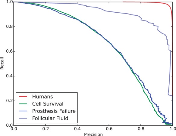
Precision/recall curves of LogReg for four MeSH: Humans, Cell Survival, Prosthesis Failure and Follicular Fluid

Fig. 3.

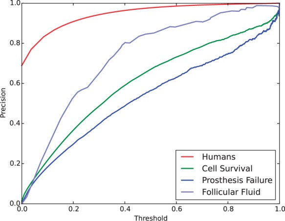
Precision of LogReg by changing threshold, for four MeSH, which were used in Figure 2

We started checking the effect of score normalization by using MetaLabeler, meaning that the performance of MLogRegN was compared with other typical, existing methods. Table 2 shows the performance of MLogRegN (and MLogReg) as well as those of several existing methods, including pattern matching, KNN and MTI. This table shows that in terms of MiF, MLogRegN achieved the highest value of 0.5754, which is followed by MTIDEF (0.5724), MTIFL (0.5624), MLogReg (0.5595), KNN (0.5213) and pattern matching. Specifically, MLogRegN outperformed MLogReg in all MiP, MiR and MiF, while this is reversed in all MaP, MaR and MaF, which validates our expectation. For example, MLogRegN achieved MiF of 0.5754 and EBF of 0.5628, while MLogReg achieved MiF of 0.5595 and EBF of 0.5502. On the other hand, MLogReg achieved MaF of 0.4612, while MLogRegN achieved MaF of 0.4335. Interestingly, MTIDEF and MTIFL achieved the best MaFs of 0.5247 and 0.5038, respectively, which means that they might be able to work well for infrequent MHs. We can also see that MTIFL is rather focused on improving precision, while MTIDEF achieved a better F-measure than MTIFL by balancing between precision and recall. For example, MTIFL achieved the highest EBP of 0.6192, while MTIDEF achieved the highest EBF of 0.5645. KNN achieved rather average performance among all methods tested in this experiment, like MiF of 0.5213, EBF of 0.5095 and MaF of 0.3927. Among the three pattern matching methods, the highest precision was obtained by using titles only, and using abstracts only achieved higher recall than using titles only, resulting in that using both titles and abstracts achieved the highest values in all three types of F-measures.

Table 2.

Performance comparison of MLogRegN with typical existing methods

Methods	MiP	MiR	MiF	EBP	EBR	EBF	MaP	MaR	MaF
MLogReg:MetaLabeler with LogReg	0.5576	0.5614	0.5595	0.5555	0.5772	0.5502	0.4600	0.4623	0.4612
MLogRegN:MLogReg with score normalization	0.5734	0.5774	0.5754	0.5702	0.5884	0.5628	0.4508	0.4175	0.4335
KNN	0.5196	0.5231	0.5213	0.5176	0.5314	0.5095	0.4142	0.3733	0.3927
Pattern matching using titles only	0.5151	0.1273	0.2041	0.5112	0.1426	0.2101	0.3444	0.1997	0.2528
Pattern matching using abstracts only	0.2315	0.2990	0.2609	0.2445	0.3117	0.2582	0.3607	0.3956	0.3773
Pattern matching using both titles and abstracts	0.2363	0.3139	0.2696	0.2498	0.3291	0.2681	0.3739	0.4153	0.3935
MTIFL	0.6142	0.5217	0.5642	0.6192	0.5386	0.5549	0.5159	0.4923	0.5038
MTIDEF	0.5740	0.5707	0.5724	0.5785	0.5909	0.5645	0.5128	0.5372	0.5247

Overall, MLogRegN achieved the highest MiF, which demonstrates the effectiveness of incorporating score normalization. Another important finding from this result is that each of all these methods shows its own unique advantage, depending on different types of evaluations, indicating that these methods can complement each other in performance. This analysis provides a good basis and reason for integrating the ideas and/or features behind these methods together.

4.5.2 Performance of MeSHRanker

We examined the performance of MeSHRanker, step-by-step, by adding different types of evidence (features) incrementally, comparing it with that of MLogRegN, which achieved the best performance in the last experiment and can be a baseline. Here, the number of MHs was predicted by MetaLabeler (Classifier B) for all compared methods. We started with checking the performance of MeSHRanker with only two types of features, i.e. MLogReg and KNN. We then added the other types of features in the order of MLogRegN, MeSH dependency, pattern matching, MeSH frequency and finally MTI, to MeSHRanker with MLogReg and KNN, checking the performance of MeSHRanker at each additional step. Table 3 shows the performance results of MLogRegN and MeSHRanker with these different types of features. This table shows that MeSHRanker with MLogReg and KNN achieved MiF of 0.5743, which is slightly lower than the baseline, which achieved a MiF of 0.5754. By incorporating MLogRegN into the features, the performance of MeSHRanker was greatly improved at MiF of 0.5899, which outperformed the baseline method, MLogRegN, already. The effect of adding MeSH dependency was also significant where the performance increase was from 0.5899 to 0.5957 for MiF, from 0.5802 to 0.5861 for EBF and from 0.4602 to 0.4938 for MaF. The large improvement in MaF indicates that incorporating MeSH dependency might have assisted finding infrequent MHs, which must have co-occurred with frequent MHs. Adding pattern matching to the features was also very helpful, which implies that pattern matching might have brought complementary information to the other features. In particular, the improvement was from 0.5957 to 0.6056 for MiF, from 0.5861 to 0.5955 for EBF and from 0.4938 to 0.5205 for MaF, also revealing the strength of pattern matching in finding infrequent MHs. Interestingly, the performance change by adding MeSH frequency was very small. This might be because the information on MeSH frequency had been already captured in the other types of features, such as KNN and MeSH dependencies. Finally, adding MTI to the features of MeSHRanker provided huge increases, resulting in the highest performance in all measures, for example, MiF of 0.6166, EBF of 0.6082 and MaF of 0.5389. Overall, we can see that the performance of MeSHRanker was highly improved by integrating multiple, different type of evidence.

Table 3.

Performance comparison of MLogRegN and MeSHRanker with different types of evidence which were incrementally added

Step	MiP	MiR	MiF	EBP	EBR	EBF	MaP	MaR	MaF
MLogRegN	0.5734	0.5774	0.5754	0.5702	0.5884	0.5628	0.4508	0.4175	0.4335
MeSHRanker (MLogReg+KNN)	0.5724	0.5763	0.5743	0.5708	0.5900	0.5637	0.4597	0.4396	0.4495
+MLogRegN	0.5878	0.5919	0.5899	0.5878	0.6072	0.5802	0.4741	0.4472	0.4602
+MeSH dependency	0.5937	0.5978	0.5957	0.5935	0.6134	0.5861	0.4889	0.4988	0.4938
+Pattern Matching	0.6036	0.6077	0.6056	0.6043	0.6242	0.5966	0.5162	0.5248	0.5205
+MeSH frequency	0.6038	0.6079	0.6059	0.6043	0.6243	0.5967	0.5166	0.5205	0.5187
+MTI	0.6145	0.6187	0.6166	0.6159	0.6363	0.6082	0.5364	0.5413	0.5389

4.5.3 Performance of MeSHLabeler

In the last experiment, the number of MHs for each target citation was predicted by MetaLabeler. Instead, in this experiment we used MeSHNumber for the ranked list of MHs, predicted by MeSHRanker with all features, and we call this combination MeSHLabeler. Also we name the final result of the last experiment, MeSHRanker (shown in the last line of Table 3). Table 4 shows the performance of MeSHLabeler and MeSHRanker, comparing it with that of MTIDEF. We note that MTIDEF is the current up-to-date indexing tool provided by NLM and the performance was already evaluated on our dataset and shown in the last line of Table 2. From Table 4, in all three types of metrics, MeSHLabeler achieved better precision while MeSHRanker achieved better recall. The only difference between MeSHRanker and MeSHLabeler was the number of predicted MHs. Thus higher precision implies that MeSHLabeler returned a smaller number of MHs with higher accuracy (precision). In terms of F-measure, MeSHLabeler achieved higher performance in both MiF and EBF, while MeSHRanker achieved higher performance in MaF, implying that infrequent MHs might be ignored by MeSHLabeler, which results in lower MaF.

Table 4.

Performance of MeSHRanker and MeSHLabeler, comparing with MTIDEF, a current cutting-edge indexing tool provided by NLM

Step	MiP	MiR	MiF	EBP	EBR	EBF	MaP	MaR	MaF
MTIDEF	0.5740	0.5707	0.5724	0.5785	0.5909	0.5645	0.5128	0.5372	0.5247
MeSHRanker	0.6145	0.6187	0.6166	0.6159	0.6363	0.6082	0.5364	0.5413	0.5389
MeSHLabeler	0.6566	0.5959	0.6248	0.6618	0.6108	0.6160	0.5450	0.5172	0.5054

Most importantly, there are two essential findings from this result: (i) MeSHRanker outperformed MTIDEF in all nine evaluation measures, and (ii) in MiF, compared with 0.5724 by MTIDEF, MeSHLabeler achieved 0.6248, which was an improvement of around 9.15% (nearly 10%).

4.6 Computational efficiency

We implemented MeSHLabeler on a server with four Intel XEON E5-4650 2.7 GHz CPU and 128 GB RAM. Most computation was spent on training the LogReg classifiers of more than 27,000 MHs, which took around 5 days. All other training parts took 1 day. However, given a new citation, annotating MeSH took only <1 s.

5 Discussion

The fundamental idea of MeSHLabeler is to integrate multiple types of diverse evidence for boosting the performance of indexing MeSH. MeSHLabeler is highly effective, showing nearly 10% improvement in both MiF and EBF over MTI, the current cutting-edge tool provided by NLM. The high performance of MeSHLabeler is derived from the diversity and accuracy of the evidence, which complement each other. MeSHLabeler uses five types of evidence: global evidence, local evidence, pattern matching, MeSH dependency and indexing rules (from MTI). The first two types of evidence are obtained by machine learning, meaning that they can be captured from the training data. The global evidence is from prediction models trained by using all instances, while the local evidence uses only similar instances to the given test instance. Pattern matching is a string matching technique that only uses the test instance. In contrast, the last two types of evidence are very different from the other evidence types. MeSH dependency is obtained from the correlation between MeSH, which requires scanning over the whole MEDLINE database. The number of combinations by different MHs is huge, which makes directly incorporating the information on different MeSH combinations very hard, and no existing methods have considered MeSH dependency. We emphasize that our strategy of capturing MeSH dependency is very efficient, resulting in high performance improvements, as shown in our experiments. We further stress that MeSHLabeler is the first method to incorporate MeSH pair correlations directly. Indexing rules from MTI are also very different from the other evidence, because they are human domain knowledge and parts of them would be very difficult to learn from data. MeSHLabeler integrates all these different types of diverse evidence, enabling MeSHLabeler to achieve high performance for MeSH recommendation.

We showed three groups of evaluation metrics, i.e. EBF, MaF and MiF. Both MiF and EBF can be higher by focusing on frequent MHs more, while MaF can be higher by considering all MHs more equally. MeSHLabeler has been developed to improve the performance of MiF, since MiF was a major metric in BioASQ challenge. For example, prediction scores of different MeSH classifiers have different accuracies (even if their values are the same, as shown in our experiments), and other methods, like MetaLabeler, have to select infrequent MHs (because of high prediction scores) more than frequent MHs. To overcome this problem, we thus incorporate the idea of score normalization in MeSHLabeler, resulting in high improvement of MiF. Also the trade-off between MiF and MaF is an issue in evaluation. For example, MeSHNumber focused on a small number of MeSH terms with high precision, and achieved a significant increase in MiF, suffering from a slight decrease in MaF.

6 Conclusion

We have presented MeSHLabeler, which achieved the best performance in the 2014 BioASQ challenge, a competition of large-scale biomedical semantic indexing. Our experiments have shown that MeSHLabeler achieved >9% increase in MiF over MTI, the current leading-edge solution provided by NLM. The most important idea of MeSHLabeler is to integrate five types of diverse evidence: global evidence, local evidence, pattern matching, MeSH dependency and indexing rules. In addition, MeSHLabeler has numerous features, such as MeSH score normalization and MeSH dependency, which have not been implemented in any other methods and greatly contributed to the better performance of MeSHLabeler. These new features might shed light on developing efficient algorithms for other multi-label classification problems with a large amount of training instances, such as ontology annotation. In the future, it would be interesting to further explore the limitations of MeSHLabeler and improve the indexing performance by combining other different types of information or evidence with the current framework, such as the prediction results of SVM.

References

- Aronson A., Lang F. (2004) An overview of MetaMap: historical perspective and recent advances. J. Am. Med. Inform. Assoc., 17, 229–236. [DOI] [PMC free article] [PubMed] [Google Scholar]
- Aronson A., et al. (2004) The NLM indexing initiative’s medical text indexer. Stud. Health Technol. Inform., 107(Pt 1), 268–272. [PubMed] [Google Scholar]
- Balikas G., et al. (2014) Results of the BioASQ track of the question answering lab at CLEF 2014. In: Working Notes for CLEF 2014 Conference, Sheffield, UK, September 1518, 2014. CEUR Workshop Proceedings 1180, CEUR-WS.org 2014, pp. 1181–1193. [Google Scholar]
- Burges C.J.C. (2010) From RankNet to LambdaRank to LambdaMART: an overview. Microsoft Research, Technical Report. [Google Scholar]
- Chang C.-C., Lin C.-J. (2011). LIBSVM: a library for support vector machines. ACM Trans. Intell. Syst. Technol., 2, 27:1–27:27. [Google Scholar]
- Fan R.-E., et al. (2008) Liblinear: a library for large linear classification. J. Mach. Learn. Res., 9, 1871–1874. [Google Scholar]
- Gu J., et al. (2013) Efficient semi-supervised MEDLINE document clustering with MeSH semantic and global content constraints. IEEE Trans. Cybern., 43, 1265–1276. [DOI] [PubMed] [Google Scholar]
- Huang M., et al. (2011a) Recommending mesh terms for annotating biomedical articles. J. Am. Med. Inform. Assoc., 18, 660–667. [DOI] [PMC free article] [PubMed] [Google Scholar]
- Huang X., et al. (2011b) Enhanced clustering of biomedical documents using ensemble non-negative matrix factorization. Inf. Sci., 181, 2293–2302. [Google Scholar]
- Jiang J., Zhai C. (2007) An empirical study of tokenization strategies for biomedical information retrieval. Inf. Retrieval, 10, 341–363. [Google Scholar]
- Jimeno-Yepes A., et al. (2012a) MEDLINE MeSH indexing: lessons learned from machine learning and future directions. In: Proceedings of the 2nd ACM SIGHIT International Health Informatics Symposium, ACM Press, pp. 737–742. [Google Scholar]
- Jimeno-Yepes A., et al. (2012b) A one-size-fits-all indexing method does not exist: automatic selection based on meta-learning. JCSE, 6, 151–160. [Google Scholar]
- Jimeno-Yepes A., et al. (2013a) Comparison and combination of several mesh indexing approaches. In: AMIA Annual Symposium Proceedings, vol. 2013 American Medical Informatics Association, p. 709. [PMC free article] [PubMed] [Google Scholar]
- Jimeno-Yepes A.J., et al. (2013b) MeSH indexing based on automatically generated summaries. BMC Bioinformatics, 14, 208. [DOI] [PMC free article] [PubMed] [Google Scholar]
- Lin J., Wilbur W. (2007) Pubmed related articles: a probabilistic topic-based model for content similarity. BMC Bioinformatics, 8, 423. [DOI] [PMC free article] [PubMed] [Google Scholar]
- Liu T. (2011) Learning to Rank for Information Retrieval. Springer, New York. [Google Scholar]
- Lu Z., et al. (2010) Evaluation of query expansion using MeSH in PubMed. Inf. Retrieval, 12, 69–80. [DOI] [PMC free article] [PubMed] [Google Scholar]
- Mao Y., Lu Z. (2013) NCBI at the 2013 BioASQ challenge task: learning to rank for automatic MeSH indexing. Microsoft Research Technical Report MSR-TR-2010-82. [Google Scholar]
- Mao Y., et al. (2014) NCBI at the 2014 BioASQ challenge task: large-scale biomedical semantic indexing and question answering. In: Working Notes for CLEF 2014 Conference, Sheffield, UK, September 15–18, 2014. CEUR Workshop Proceedings 1180, CEUR-WS.org 2014, pp. 1319–1327. [Google Scholar]
- Mork J., et al. (2013) The NLM medical text indexer system for indexing biomedical literature. In: BioASQ@ CLEF. Proceedings of the first Workshop on Bio-Medical Semantic Indexing and Question Answering, a Post-Conference Workshop of Conference and Labs of the Evaluation Forum 2013 (CLEF 2013), Valencia, Spain, September 27th, 2013. CEUR Workshop Proceedings 1094, CEUR-WS.org 2013. [Google Scholar]
- Mork J., et al. (2014) Recent enhancements to the NLM Medical Text Indexer. In: Working Notes for CLEF 2014 Conference, Sheffield, UK, September 1518, 2014. CEUR Workshop Proceedings 1180, CEUR-WS.org 2014, pp. 1328–1336. [Google Scholar]
- NCBI Resource Coordinators (2015) Database resources of the national center for biotechnology information. Nucleic Acids Res., 43(Database issue), D6–D17. [DOI] [PMC free article] [PubMed] [Google Scholar]
- Nelson S.J., et al. (2004) The MeSH translation maintenance system: structure, interface design, and implementation. Stud. Health Technol. Inform. , 11(Pt 1), 67–69. [PubMed] [Google Scholar]
- Partalas I., et al. (2013) Results of the first BioASQ workshop. In: BioASQ@ CLEF. Proceedings of the first Workshop on Bio-Medical Semantic Indexing and Question Answering, a Post-Conference Workshop of Conference and Labs of the Evaluation Forum 2013 (CLEF 2013), Valencia, Spain, September 27th, 2013. CEUR Workshop Proceedings 1094, CEUR-WS.org 2013, pp. 1–8. [Google Scholar]
- Ruch P. (2006) Automatic assignment of biomedical categories: toward a generic approach. Bioinformatics, 22, 658–664. [DOI] [PubMed] [Google Scholar]
- Stokes N., et al. (2010) Exploring criteria for successful query expansion in the genomic domain. Inf. Retrieval, 12, 17–50. [Google Scholar]
- Tang L., et al. (2009) Large scale multi-label classification via metalabeler. In: Proceedings of the 18th international conference on World wide web. ACM Press, New York, NY, USA, pp. 211–220. [Google Scholar]
- Trieschnigg D., et al. (2009) MeSH Up: effective MeSH text classification for improved document retrieval. Bioinformatics, 25, 1412–1418. [DOI] [PMC free article] [PubMed] [Google Scholar]
- Tsoumakas G., et al. (2013) Large-scale semantic indexing of biomedical publications. In: BioASQ@ CLEF. Proceedings of the first Workshop on Bio-Medical Semantic Indexing and Question Answering, a Post-Conference Workshop of Conference and Labs of the Evaluation Forum 2013 (CLEF 2013), Valencia, Spain, September 27th, 2013. CEUR Workshop Proceedings 1094, CEUR-WS.org 2013. [Google Scholar]
- Zhang M., Zhou Z. (2014) A review on multi-label learning algorithms. IEEE Trans. Knowl.Data Eng., 26, 1819–1837. [Google Scholar]
- Zhu S., et al. (2009a) Enhancing MEDLINE document clustering by incorporating mesh semantic similarity. Bioinformatics, 25, 1944–1951. [DOI] [PubMed] [Google Scholar]
- Zhu S., et al. (2009b) Field independent probabilistic model for clustering multi-field documents. Inf. Process. Manage., 45, 555–570. [Google Scholar]