Reconstructing 16S rRNA genes in metagenomic data

Abstract

Metagenomic data, which contains sequenced DNA reads of uncultured microbial species from environmental samples, provide a unique opportunity to thoroughly analyze microbial species that have never been identified before. Reconstructing 16S ribosomal RNA, a phylogenetic marker gene, is usually required to analyze the composition of the metagenomic data. However, massive volume of dataset, high sequence similarity between related species, skewed microbial abundance and lack of reference genes make 16S rRNA reconstruction difficult. Generic de novo assembly tools are not optimized for assembling 16S rRNA genes. In this work, we introduce a targeted rRNA assembly tool, REAGO (REconstruct 16S ribosomal RNA Genes from metagenOmic data). It addresses the above challenges by combining secondary structure-aware homology search, zproperties of rRNA genes and de novo assembly. Our experimental results show that our tool can correctly recover more rRNA genes than several popular generic metagenomic assembly tools and specially designed rRNA construction tools.

Availability and implementation: The source code of REAGO is freely available at https://github.com/chengyuan/reago.

Contact: yannisun@msu.edu

1 Introduction

Microbes are ubiquitous species existing in all environments on earth, including extreme conditions (Rothschild and Mancinelli, 2001). From the desert to acid wastewater, from pine forest soil to mine drainage, they sustain themselves using various mechanisms (Konings et al., 2002). Human bodies are also habitats of microbes. It is estimated that there are 10¹⁴ bacterial cell inhabiting on our body, which is 10 times more than our own cells (Berg, 1996; Savage, 1977). Human life as well as the entire ecosystem are profoundly affected by microbes. There is a strong need to understand the function of microbial communities and how they interact with their hosts. The function of microbial community is defined by its composition and diversity (Loreau et al., 2001). In particular, metagenomic data, which contains sequenced DNA reads of uncultured microbial species from environmental samples, provide a unique opportunity to thoroughly analyze microbial species that have never been identified before.

A commonly adopted approach for identifying the microbial species in environmental samples is to conduct comparative analysis of ribosomal RNA sequences (Woese and Fox, 1977; Woese et al., 1990). The use of rRNA for microbial phylogenetic analysis had become such a relied-upon methodology that by 2008; 77% of all INSDC (Benson et al., 2010; Cochrane et al., 2009; Tateno et al., 2002) bacterial DNA sequence submissions described an rRNA gene sequence (Christen, 2008)! 16S rRNA reads from metagenomic studies provide a source of sequences that are not subject to PCR primer bias and therefore covers taxa that might be missed by existing popular primer sets (Hamady and Knight, 2009). The rRNA genes are a patchwork of hypervariable (rapidly evolving) and universally conserved regions. Unassembled reads in metagenomic data usually lack usable phylogenetic signal. Thus, there is a strong need to recover complete or near-complete rRNA genes from the short reads for analyzing microbial composition in the underlying samples. However, the massive data volume, short read length, skewed species abundance and high similarity of 16S rRNA genes all make rRNA recovery in metagenomic data very difficult. The goal of this work is to provide a tool that can efficiently and accurately recover rRNA genes from metagenomic data.

Existing pipelines for annotating rRNA genes in metagenomic data can be divided into two groups. The first type of pipelines relies on existing de novo assembly tools to output assembled contigs, which are then used as input to available genome-wide rRNA search tools. There are various metagenomic assembly programs (Laserson et al., 2011; Luo et al., 2012; Namiki et al., 2012; Peng et al., 2011; Salzberg et al., 2008; Treangen et al., 2013; Wu et al., 2012), which intend to recover individual genomes in an environmental sample. Metagenomic assembly is computationally difficult (Treangen et al., 2013). In particular, previous work shows that metagenomic sequencing of high-complexity microbial communities results in little or no assembly of reads (Jeffrey and Zhong, 2011; Tringe et al., 2005). In addition, our goal is to detect rRNA genes in metagenomic data while much of generic de novo assemblies consist of other genomic regions. Thus, the commonly used pipeline of combining generic metagenomic assembly and genome-wide rRNA detection tools is convenient but not optimized for rRNA detection in metagenomic data. The second type of pipelines avoids metagenomic assembly and incorporates properties of rRNA genes (Fan et al., 2012; Miller et al., 2011). The most promising one is perhaps EMIRGE (Miller et al., 2011), which uses an expectation maximization approach along with a set of reference gene sequences to assemble rRNA genes from metagenomic data. However, EMIRGE requires a large number of known rRNA genes for the mapping step and may miss remotely related rRNA genes.

Therefore, lacking reference genomes, recovering full-length rRNA genes from a large number of short and error-prone reads is still an outstanding challenge. In this work, we propose and implement a targeted rRNA assembly program, REAGO, which is optimized for rRNA gene recovery in metagenomic data. It has three advantages comparing with existing methods. First, it significantly reduces the problem size by first discarding reads that are not likely sequenced from rRNA genes. Second, paired-end information is carefully applied to guide gene assembly and thus distinguish rRNA genes from different species. Third, the profile-based homology search step enables us to decide the orientation and relative position of each contig, leading to efficient scaffolding. We applied our tool to two metagenomic datasets and benchmarked its performance with several other programs. The experimental results show that our tool competes favorably in recovering rRNA genes in metagenomic datasets.

2 Method

2.1 Overview of REAGO

Figure 1 is a schematic representation of the pipeline, which contains four stages. First, we identify 16S rRNA reads from the original metagenomic dataset using secondary-structure-aware homology search. The majority of non-16S reads are discarded in this process, significantly reducing the problem size. Second, REAGO constructs overlap graphs. Various graph reduction techniques are applied to remove possible sequencing errors and prepare the graph for efficient assembly. The third stage assembles reads into contigs by our path finding algorithms. The path finding procedure is guided using paired-end information and aims to avoid generating chimeric 16S rRNA genes by maximizing Weighted Paired-End Match Score (WPEMS) (Section 2.5). Finally, paired-end information again is used to scaffold incomplete 16S fragments, if any, into longer contigs or full-length genes.

Fig. 1.

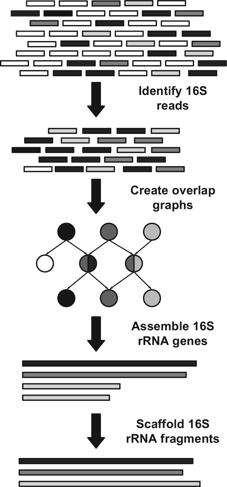
Pipeline of the 16S rRNA gene assembly. Short black and gray bars represent reads originating from different 16S rRNA genes. Short white bars represent reads from non-16S regions. Long bars represent contigs assembled from short reads

2.2 16S rRNA reads identification

In our method, we first conduct homology search to identify reads originating from 16S rRNA genes. To utilize both the sequence and structural conservation of 16S rRNA genes, we align metagenomic reads to a Stochastic Context-Free Grammar (SCFG) based model (Durbin, 1998), which is trained on characterized rRNA genes and describes both the sequence and secondary structure conservation. The-state-of-the-art implementation of SCFG is covariance model (CM) in Infernal (Nawrocki et al., 2009). The scores and associated E-values of the alignments between reads and the CM are used to screen rRNA reads. In general, reads sequenced from 16S rRNA genes are likely to get high alignment scores while reads from other genes tend to receive low scores.

Fragmentary sequences pose great challenges to the alignment algorithms since structural information in short reads is likely to be partially missing. As a result, such short reads tend to receive marginal alignment scores and are not identified. Infernal handles this problem by recovering possibly missing bases while performing the alignment (Kolbe and Eddy, 2009). Thus, short 16S rRNA reads can still receive significant alignment scores.

BLAST (Altschul et al., 1990) is another choice for 16S read identification. By aligning reads with the reference 16S rRNA database, rRNA reads may be recognized using BLAST alignment scores or E-values. We choose SCFG-based homology search over BLAST for two reasons. First, BLAST conducts homology search based on sequence similarity and may miss reads lacking primary sequence conservation. 16S ribosomal RNAs share high sequence similarity on many regions across different species. However, there also exist a number of variable regions where secondary structures are better conserved than primary sequences. Secondary structural information could then be very helpful to provide additional evidence for 16S sequence identification. A number of studies have demonstrated the advantages of incorporating secondary structural information in various types of non-coding RNA homology search (Nawrocki et al., 2009). Experiments were conducted to compare BLAST and CM-based approaches (Kolbe and Eddy, 2009; Yuan and Sun, 2013) on identifying short rRNA reads. The results indicate that BLAST tends to miss short rRNA reads that are sequenced from non-conserved regions. CM-based approaches generally improve the identification accuracy by including secondary structure information. The second reason behind choosing SCFG-based homology is that the single SCFG-based model provides a convenient reference for inferring the orientation and relative positions among contigs during the scaffolding stage.

2.3 Overlap graph creation and graph pruning

All reads that are possibly sequenced from rRNA genes are used to construct an overlap graph for assembly. An overlap between two reads is formed if the suffix of a read matches the prefix of another read. A straightforward overlap detection method performs pair-wise comparison among all reads, requiring $O(n^2)$ comparisons. There exist efficient implementations of overlap graphs based on data structures such as hash table and BTW (Gonnella and Kurtz, 2012; Simpson and Durbin, 2012). We choose Readjoiner (Gonnella and Kurtz, 2012), which provides a set of time and space efficient algorithms for detecting all suffix-prefix matches among a set of reads. In overlap graphs, each vertex represents a read and each edge represents a suffix-prefix match of size at least l, a pre-determined overlap threshold. l has high impact on complexity and connectivity of graphs. Small l tends to increase the connectivity, but also complexity, of the overlap graph. Larger l is likely to produce less tangled graph, but can possibly miss connections between reads from lowly sequenced regions. Note that transitive edges are automatically removed in the output by Readjoiner.

The original graphs generated from the output of Readjoiner could be very complex because of the large data size, sequencing errors, and highly similar regions shared by different genes. We apply an iterative graph pruning procedure, as depicted in Figure 2, to gradually simplify the graph at each iteration. The procedure terminates when the graph stops changing. Below we detail each stage.

Fig. 2.

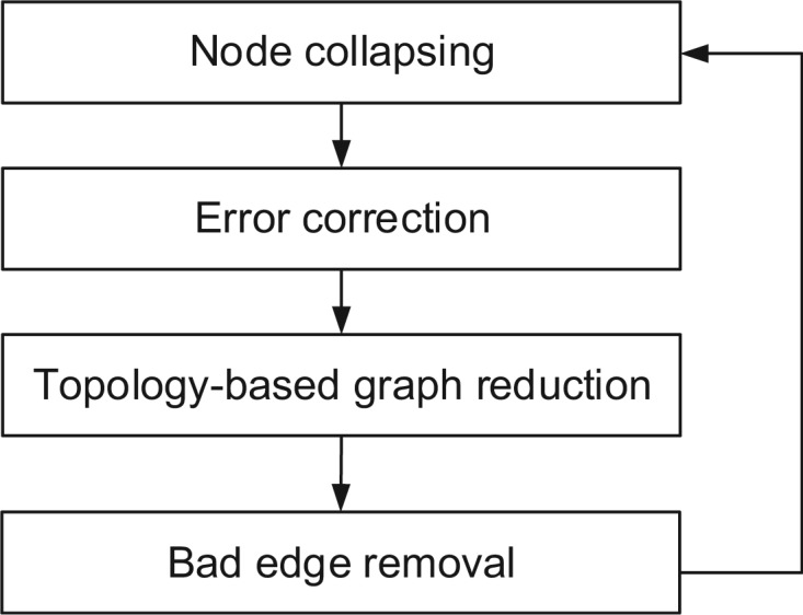
Graph reduction is conducted iteratively until there is no change on the graph

2.3.1 Node collapsing

The original overlap graph tends to have chains of linearly connected vertices. In such chains, each vertex has only a single incoming edge and outgoing edge. Such vertices can be merged without loss of reachability.

2.3.2 Alignment-based error correction

Sequencing errors and highly similar regions shared by different genes can contribute to a large number of bifurcations, greatly complicating the graph. Error correction in metagenomic data is an unsolved problem. Rare reads may come from low abundance genes rather than sequencing errors. Nevertheless, we still follow the error correction rationale commonly used in de novo genome assembly and correct bases in rare reads. As shown in Figure 3, we applied a heuristic but efficient alignment-based error correction to two types of bifurcations. Reads or contigs from sibling nodes $V_0,V_1,\cdots ,V_n$, which share the same predecessor or successor, are aligned. Specifically, based on the known overlaps with the contig in the common predecessor or successor, the contigs in the sibling nodes will be aligned first. Then the reads inside the contigs can be aligned using their positions inside the contig.

Fig. 3.

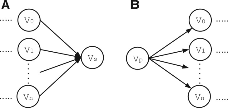
Two types of bifurcation where error correction is applied. (A) Multiple vertices sharing the same successor. (B) Multiple vertices sharing the same predecessor

For each column in the read alignment, a base is corrected if it is overwhelmingly out-voted by other bases that are aligned to it. An assumption made here is, if a base is sequenced multiple times, it is correctly sequenced the majority of the time. A base a is corrected into $a\prime$, if and only if the number of $a\prime$ is at least τ times more than the number of a. It is worth noting that this strategy could potentially incorrectly mutate bases from low abundance genes, since the number of those bases could be out-voted by bases from related and abundant genes. In order to make our tool more practically useful, we sacrifice some accuracy for assembly efficiency. The value of τ is customizable so the user can change the strictness of error correction in different datasets by adjusting the value of τ. A larger τ tends to yield more conserved error correction. A smaller τ tends to correct more erroneous bases, but may also falsely modify correct bases into incorrect ones, especially in regions with low coverage.

An example is depicted in Figure 4. Sequences represented in vertices V₂ and V₃ are very similar and only differ in one base. The bifurcation may be caused by sequencing error or simply represent similar regions from highly related species. Reads in both vertices are aligned. In the highlighted column, the number of base T in V₃ is far less than that of the base A in V₂, so we mutate the T into A then merge V₂ and V₃ in to a single vertex.

Fig. 4.

An example of error correction (applied on V₂ and V₃). The sequence represented by each node is given beside the node. (A) Ungapped alignment of reads from bifurcating vertices. (B) Mutate rare bases. (C) Remove bifurcation

2.3.3 Topology-based graph reduction

Alignment-based error correction is only applied to nodes sharing the same predecessor or successor. Following the existing assembly methods (Zerbino and Birney, 2008), we conduct topology-based graph reduction and remove tips and bubbles. Similar to the bifurcation removal procedure, the tip and bubble removal could potentially remove contigs from low abundance genes. So we also allow the thresholds used in this step to be adjusted by users.

2.4 Bad edge removal

Due to the nature of metagenomic datasets, there may exist multiple species with very high sequence similarity. Thus, reads originating from different species have high chance to form edges in the graph. In another word, having suffix-prefix match does not necessarily guarantee correct connection. Wrong edges not only increase the complexity of graph but also lead to chimera.

Thus after graph reduction, we applied a Naive Bayes Classifier, similarly to the RDP classifier (Wang et al., 2007), on each vertex and approximately annotate it with one or more genera. If the vertices on either end of an edge do not share any common annotated genus, we regard it as a ‘bad’ edge and remove it. Annotation of each vertex can be obtained by calculating a posterior probability $P(G_i|C)$, where C is the contig that the vertex represents and G_i represents a genus. The probability indicates the likelihood that C originated from G_i. If the probability is higher than a threshold, we annotate C with G_i. To calculate $P(G_i|C)$, we first decompose the contig C into a set of k-mers $k_1,k_2,\dots ,k_n$. Same as the RDP classifier, the default value of k is 8. Then $P(C|G_i)$ can be extended as $P(k_1,k_2,\dots ,k_n|G_i)$. Assuming the independence of k_i as in the Naive Bayes Classifier, we can further simplify the likelihood to $P(k_1|G_i)P(k_2|G_i)\cdots P(k_n|G_i)$, in which each term can be pre-calculated based on the RDP database (Cole et al., 2005). The prior probability $P(G_i)$ can also be calculated as the proportion of sequences in G_i to the total number of sequences in the RDP database. The posterior probability $P(C|\overline{G_i})$, which indicates the likelihood that C does not originate from G_i, can also be calculated in the same way. The detailed steps are listed in Figure 5.

Fig. 5.

The detailed calculation of the probability that a contig C originated from a genus G_i

For a vertex, a genus G_i is included into its annotation if $P(G_i|C)$ is greater than a threshold. As most vertices in the graphs represent only short and partial 16S genes, the classifier may not have enough evidence to uniquely and accurately annotate them. As a result, each vertex is generally associated with multiple genera. Yet, base on our observation, the annotation always includes the true positive genus. The edge removal algorithm works better on longer sequences. Thus, it is iteratively applied after graph reduction and node collapsing, as shown in Figure 2.

2.5 Guided path finding using paired-end information

We then recover 16S rRNA sequences by finding paths that represent a full or partial rRNA gene. Path finding starts at a vertex with no incoming edge and terminates at a vertex with no outgoing edge. Paired-end information of reads are widely used in many assembly tools for guiding the creation of contigs (Zhang et al., 2014) or scaffolds. The rationale is that the two ends of a read pair should be assembled in the same contig or scaffold. To utilize the paired-end information, a common approach adopted by SOAPdenovo (Li et al., 2010), ABySS (Simpson et al., 2009) and ALLPATHS (Butler et al., 2008) creates graphs from a set of contigs where each vertex represents a contig and an edge is formed between two vertices if more than a certain number of read pairs exist between their reads. Then the graphs are searched, using various constraints and heuristics, to extend contigs into longer scaffolds. Velvet (Zerbino and Birney, 2008), on the other hand, assumes a small variance of insert size distribution and aims to create ‘long nodes’ that are longer than all inserts. The objective function intends to maximize the number of ‘long nodes’ while minimizing the number of read pairs spanning over such nodes. As an extension of Velvet, MetaVelvet (Namiki et al., 2012) uses paired-end information to guide the creation of contigs by checking their consistency. The number of paired-end reads connecting the origin node and the extension node is used to resolve chimeric node candidates.

In our algorithm, we use paired-end information to guide the path finding and scaffolding. At each vertex with multiple successors, we decide which one to include based on a new metric, WPEMS, which gives higher weights to paired-end reads located in distant nodes than those located in nearby nodes. Let $(r,r\prime )$ be a mate pair located in vertices V and $V\prime$ ($V\ne V\prime$), respectively. The WPEMS of this read pair is thus $2^{d(r,r\prime )}$, where $d(r,r\prime )$ is the number of vertices between V and $V\prime$. If $V=V\prime$, we define its WPEMS as 0. The WPEMS of a path P is the sum of WPEMS of all paired end reads in P.

$$\text{WPEMS}(P)={\displaystyle \sum _{(r,r\prime )}{2}^{d(r,r\prime )}}$$

When deciding among a set of vertices to visit next, we select the vertex that maximizes the WPEMS of the current path in a greedy way. The rationale behind the design of WPEMS is that only read pairs existing in non-adjacent vertices provide extra evidence for path finding. Read pairs included in the same vertex or spanning adjacent vertices do not provide additional path finding information beyond the existing overlap graph. In practice, the graph pruning procedure (Fig. 2) leads to many vertices representing relatively long contigs. Thus, for average fragment sizes such as hundreds of bases, the paired-end reads usually exist within the same vertex or vertices already connected by an edge. Figure 6 describes a typical example of read pair distribution in a graph. There are usually many paired-end reads spanning adjacent vertices such as from n₆ to n₈. Many fewer paired-end reads span non-adjacent vertices, such as those from n₁ to n₇ and from n₄ to n₇. Paired-end reads located in two adjacent nodes have WPEMS of 1, because there is no intermediate node between the adjacent nodes.

Fig. 6.

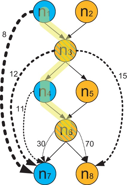
Path finding using paired-end information. Solid lines represent overlaps between nodes and dashed lines represent the existence of paired-end reads. The numbers beside dashed lines are the numbers of paired end reads between the corresponding nodes

We use the example in Figure 6 to explain our path finding procedure. Nodes in the graph are formed by reads from two different 16S rRNA genes A and B, colored in blue and yellow, respectively. Nodes n₃ and n₆ are represented using shaded color since they are formed by reads from common regions of A and B. Genes A and B are represented by $n_1\to n_3\to n_4\to n_6\to n_7$ and $n_2\to n_3\to n_5\to n_6\to n_8$, respectively. Suppose the path finding process has successfully identified the path $n_1\to n_3\to n_4\to n_6$, which is highlighted in yellow, and needs to choose between n₇ and n₈ as the next node to include. By choosing n₇, the increased score is $8\times 2^3+12\times 2^2+11\times 2^1+30\times 2^0=164$. By choosing n₈, the score is $15\times 2^2+70\times 2^0=130$. Thus, WPEMS will choose n₇, the correct node, because of more paired-end reads shared between non-adjacent nodes.

In order to produce all 16S ribosomal RNA sequences, we apply the path finding algorithm on each vertex with no incoming edge. If the length of a contig represented by a path is greater than a user-defined threshold, we consider the contig to be a full-length gene. Otherwise, we include it in the input to the next scaffolding stage. As this approach is a greedy algorithm, the time complexity is very low. The entire path finding procedure take O(mn) time to complete, where m is the average out-degree of each vertex and n is the average distance between nodes with no incoming edge and nodes with no outgoing edge.

2.6 Scaffolding 16S rRNA segments

In the path finding stage, contigs longer than a user-defined parameter L, are output directly. Contigs shorter than L are selected for further processing. Short contigs are usually created due to regionally low coverage of rRNA genes in metagenomic data. Reads from lowly sequenced regions failed to create connection to other region due to small overlap. As a result, rRNA segments originating from the same gene may be broken apart. To produce full-length rRNA sequences, we can utilize the WPEMS, with a minor modification, to scaffold shorter segments. First, as we know the orientation and alignment position of each read on the CM during the homology search, we can infer the orientation and alignment position of each contig based on the contained reads. Then, for two segments S_A and S_B with S_A being in the upstream of S_B (Fig. 7), the WPEMS between S_A and S_B is defined as

$$\text{WPEMS}(S_A,S_B)={\displaystyle \sum _{(r,r\prime )}{2}^{d(r,r\prime )}}$$

where $(r,r\prime )$ is a mate pair. r and $r\prime$ are in S_A and S_B, respectively. As we have no information about the gap between S_A and S_B, we define $d(r,r\prime )$ as the total number of vertices after r and before $r\prime$, in S_A and S_B, respectively. An example is given in Figure 7.

Fig. 7.

Calculate the score between two segments. Arcs indicate existence of paired-end reads between vertices. Thickness of arcs indicate weight of the paired-end match. Actual weights are labeled beside each arc. Assuming there is only one mate-pair among contigs, the WPEMS is 22

We only calculate $\text{WPEMS}(S_A,S_B)$ if S_A is on the upstream of S_B and their CM alignment position overlap. If S_A and S_B are from the same gene, $\text{WPEMS}(S_A,S_B)$ tends to be the highest among all $\text{WPEMS}(S_A,S_i)$ and $\text{WPEMS}(S_j,S_B)$. So we calculate the pair-wise WPEMS in all segments. We then connect S_A and S_B, if

$$\text{WPEMS\hspace{0.5em}}(S_A,S_B)>\text{WPEMS\hspace{0.5em}}(S_A,S_i)$$

$\text{for\hspace{0.5em}all\hspace{0.5em}}{S}_i\text{\hspace{0.5em}on\hspace{0.5em}the\hspace{0.5em}downstream\hspace{0.5em}of\hspace{0.5em}}{S}_A,\text{\hspace{0.5em}and}$

$$\text{WPEMS}(S_A,S_B)>\text{WPEMS}(S_j,S_B)$$

$\text{for\hspace{0.5em}all\hspace{0.5em}}{S}_j\text{\hspace{0.5em}on\hspace{0.5em}the\hspace{0.5em}upstream\hspace{0.5em}of\hspace{0.5em}}{S}_B$

All connected segments with total length longer than L will be output.

3 Experimental results

To evaluate the performance of our algorithm, we applied REAGO to a simulated metagenomic dataset and a mock community dataset. As the species and their genomes are largely known in the two datasets, we are able to evaluate the accuracy of rRNA assembly. We benchmarked our tool with EMIRGE, a 16S rRNA identification tool, and two popular metagenomic assembly tools, IDBA-UD (Peng et al., 2012) and MetaVelvet (Namiki et al., 2012). We also compared the performance of the three tools on two sets of inputs, the entire datasets and only true positive reads (i.e. reads sequenced from 16S rRNA genes). For all the tools, we evaluated their performance to reconstruct 16S rRNA sequences at sequence-level and genus-level. We also recorded and compared their running time on the same high performance computing node with a 64-bit CPU and Linux operating system. The detailed commands, parameters and output can be found along with the source code of REAGO.

3.1 Experiment 1: simulated metagenomic dataset

To evaluate the performance of REAGO, we first applied it to a simulated metagenomic dataset containing reads from 11 species of 8 genera. We used WGSIM (Li, 2011) to generate 9.6e+7 paired-end, 110 nt long error-containing reads. The sequencing error rate was set to 2% by default and the insert size was set to 320 with a standard deviation of 10 bases. The relative abundance of the 11 species is shown in Table 1. The most abundant species is 11 times more abundant than the least abundant species.

Table 1.

Species abundance

Species	Abundance (%)
Bacteroides thetaiotaomicron VPI-5482 (BTV)	24.17
Bacteroides vulgatus (BVG)	4.13
Chlorobium phaeobacteroides DSM 266 (CPB)	10.02
Chlorobium phaeovibrioides DSM 265 (CPV)	6.29
Chlorobium tepidum TLS (CTT)	12.38
Salinispora tropica CNB-440 (STC)	1.96
Sulfurihydrogenibium sp YO3AOP1 (SSY)	4.72
Bordetella bronchiseptica RB50 (BBR)	7.86
Burkholderia xenovorans LB400 (BXL)	10.02
Leptothrix cholodnii SP-6 (LCS)	4.72
Nitrosomonas europaea ATCC 19718 (NEA)	13.75

To challenge REAGO, we selected some closely related species in the same genus with highly similar 16S rRNA genes. We listed their pair-wise sequence similarity in Table 2. For example, three selected species in Chlorobium share sequence identity above 93%. Chlorobium phaeobacteroides and Chlorobium phaeovibrioides even share similarity as high as 96%. Reads simulated from these species tend to produce extremely tangled overlap graphs that pose challenges for assembly. Traversing such graphs will result in a large number of paths, and most of which represent chimeric assemblies.

Table 2.

Pair-wise sequence similarity

	BBR	BTV	BVG	BXL	CPB	CPV	CTT	LCS	NEA	SSY	STC
BBR	-	-	-	-	-	-	-	-	-	-	-
BTV	71	-	-	-	-	-	-	-	-	-	-
BVG	71	91	-	-	-	-	-	-	-	-	-
BXL	91	72	71	-	-	-	-	-	-	-	-
CPB	76	75	75	75	-	-	-	-	-	-	-
CPV	75	75	75	74	96	-	-	-	-	-	-
CTT	75	75	74	74	93	94	-	-	-	-	-
LCS	90	73	72	90	76	77	76	-	-	-	-
NEA	88	73	72	89	75	75	74	86	-	-	-
SSY	73	72	72	73	73	73	73	74	74	-	-
STC	76	72	71	76	77	77	76	77	76	76	-

Bold numbers indicate sequence similarity above 90%.

3.1.1 Performance of rRNA reads classification

Following the pipeline in Figure 1, we applied cmsearch, CM alignment program in Infernal to identify reads originating from rRNA genes. When building the CM for cmsearch, we only used rRNA genes that are not in the simulated dataset. Specifically, we downloaded 2591 bacterial 16S rRNA genes from the RDP website (Cole et al., 2005). Then we removed the rRNA genes in the 11 species used for simulation and also the ones in the same genera as those 11 species. As a result, we have 2537 genes in the training set for building the CM in cmsearch. The performance of cmsearch is quantified using two metrics: sensitivity and positive predictive value (PPV). The set of reads sequenced from 16S rRNA genes are true positive (i.e. TP) while the set of reads extracted from other regions are true negative. Let P be the set of reads predicted as positive by cmsearch. We thus have

$$\begin{array}{l}\text{sensitivity}=\frac{P\cap TP}{TP}.\\ PPV=\frac{P\cap TP}{P}\end{array}$$

It is worth noting that we only keep reads that can be globally aligned to CM. For reads that are partially sequenced from the rRNA genes and thus produce partial or local alignments, we don’t keep them for downstream analysis. Correspondingly, during the performance evaluation, we only use reads that are completely sequenced from the rRNA genes and non-rRNA regions. Reads sequenced from boundaries of rRNA genes will not be used for computation. For this simulated dataset, the sensitivity and PPV of cmsearch in recognizing rRNA reads are both 0.990. Reads originating from 16S rRNA genes were precisely separated from those from other regions of genomes with only a small amount of incorrectly classified reads. The output of cmsearch contains 82 638 reads, which are used as input for overlap graph construction. Compared with the original size of the dataset (9.6e7 reads), the problem size is significantly reduced.

3.1.2 Overlap graph construction

The reads classified as rRNA reads by cmsearch were used as input to Readjoiner for efficient overlap graph construction. By default, the overlap threshold was set to 70% of the read length, which is 77 in the simulated dataset. A larger overlap may be used when sequencing depth is high for each species, while smaller overlap should be used if some low abundance species are present. A smaller overlap, however, tends to yield more tangled graphs. We have tried a range of overlaps from 66 to 99. The results are almost identical on the simulated dataset. The default error correction threshold τ was set to 50, indicating that a base will be corrected if at least 50 bases of a different kind are aligned to it.

We evaluated the efficiency of our error correction and graph reduction algorithms using the change of graph complexity, which is quantified by the total number of paths in the graph. The increase of the number of different paths implies the increase of the graph complexity. We only record ‘complete’ paths that start at nodes with no incoming edge and end at nodes with no outgoing edges. The original graph contains 16 994 765 paths. After applying our graph reduction procedures, the graph is significantly simplified, containing only 961 paths. As shown by the assembly results presented in the following section, a majority of the genes have been kept in the reduced graph.

3.1.3 Assembly

Finally, we evaluated the performance of our assembly algorithms and compared it with EMIRGE, IDBA-UD and MetaVelvet. Metrics used are the number of genes recovered at sequence level, the number of genera recovered, the number of falsely recovered genes, and the running time. For all tools, all contigs or super-contigs longer than 1350 nts are considered to be final output. An assembly is considered to be correct at sequence level if and only if it can be aligned to the true gene with at least 98% identity by BLAST. A genus is correctly recovered as long as one of its genes is recovered.

For EMIRGE we did two experiments using two different rRNA gene databases. The first one is its original small subunit ribosomal RNA (SSU) candidate database excluding just the 11 training genes. Similar to the method of constructing the training set for the CM in REAGO, the second one uses the original database excluding all genes in the eight selected genera. All parameters of IDBA-UD were set as default. For MetaVelvet, we followed the recommendation in its tutorial and used k-mer size of 55.

As displayed in Table 3, our assembly algorithms demonstrate better performance in reconstructing 16S rRNA genes. EMIRGE achieved the same sensitivity as our tool with the first database. But it took much longer running time. For the second database, which excluded all genes in the eight chosen genera as the training set for our tool, it recovered many fewer genes. Thus, if a genus in a metagenomic dataset does not exist in the SSU candidate database at all, it is possible that the genes from this genus cannot be recovered. IDBA-UD was correct only on three genes and MetaVelvet only identified one. The results show that generic de novo assembly tools are not optimized for recovering 16S rRNA genes and thus are not recommended for this task.

Table 3.

Performance of 16S rRNA gene recovery

Tool	# output genes	# genes recovered	# genera recovered	# incorrect assemblies	Running time
REAGO	12	11/11	8/8	1	4:53:19
EMIRGE, 16S DB, excluding the 11 genes	16	10/11	7/8	6	96:12:1
EMIRGE, 16S DB, excluding eight genera	23	6/11	5/8	17	96:14:29
IDBA-UD	416	3/11	3/8	413	16:36:28
MetaVelvet	1 258	1/11	1/8	1 257	5:35:30

In all tables hereafter, ‘# output genes’ is the number of outputs longer than 1 350 nts. The CM used in REAGO is trained on 16S rRNA genes excluding all in the eight genera of the test data.

The performance of REAGO heavily relies on two key steps: rRNA read homology search and de novo assembly. Our pipeline allows the users to replace the assembly component with other generic assembly tools or rRNA construction tools. To evaluate whether our assembly step contributes to the improvement of REAGO over other tools, we applied EMIRGE, IDBA-UD and MetaVelvet directly on true positive 16S reads. Compared to applying homology search to recognize rRNA reads, using only true positive rRNA reads ensures that the tested tools obtain the optimal rRNA assembly/construction results. As summarized in Table 4, even using this ideal input, the rRNA construction performance of the three tools are not better than REAGO (Table 3), demonstrating the advantages of the assembly stage of REAGO. Table 4 also shows that the performance of all tools improve when using only rRNA reads as input. As expected, they all run significantly faster and produce fewer contigs. When using the database excluding 11 genes, EMIRGE achieves similar performance to REAGO, except outputting four more wrong assemblies. However, when excluding all genes in the eight genera as we did for REAGO, it is worse than REAGO.

Table 4.

Performance of 16S rRNA gene recovery using only true positive reads as input

Tool	# output genes	# genes recover	# genera recovered	# incorrect assemblies	Running time
REAGO	12	11/11	8/8	1	0:2:14
EMIRGE, 16S DB, excluding the 11 genes	17	11/11	8/8	5	0:13:01
EMIRGE, 16S DB, excluding the 8 genera	21	7/11	6/8	14	0:14:10
IDBA-UD	3	3/11	3/8	0	0:5:26
MetaVelvet	1	1/11	1/8	0	0:0:35

3.2 Experiment 2: synthetic metagenomic data

To further assess the performance of our assembly algorithms, we applied REAGO to a metagenomic dataset (SRR606249) sequenced from an archaeal and bacterial synthetic community (Shakya et al., 2013), which contains 16 archaeal species and 48 bacterial species, covering 50 different genera. The metagenomic dataset was sequenced using Illumina HiSeq-2000 and contains ∼11.1 Gbp in total. Reads in the dataset are all 101-base long and were sequenced in pairs. The annotations of 16S rRNA genes in these species were downloaded from NCBI. High sequence similarity exists among genes in the same genus and genes across different genera. For instance, species from Leptothrix, Bordetella, Burkholdera and Nitrosomonas share sequence similarity above 97%. Three species under Thermotoga share sequences similarity above 99%. Additionally, the abundance of species is more skewed in this dataset than in the first one. The most abundant species is over 20 times more abundant than the least abundant species.

3.2.1 rRNA reads classification

We applied cmsearch for rRNA homology search. As this dataset contains both archaeal and bacterial species, we trained two types of CMs using genes in archaeal and bacterial species, respectively. In addition, for each type of CM, we constructed two CMs using two training sets. The first CM was trained on all 16S genes from RDP excluding the exact copies of rRNA genes from the 64 species of the synthetic community. Next, we further removed all genes belonging to any of the 50 genera and trained the second CM. The read mapping results and the annotation of the 16S rRNA genes in the component genomes enable us to determine whether a read is part of an rRNA gene. In this dataset, there are 67 979 reads completely sequenced from rRNA genes. Based on the known origins of the reads, we can evaluate the performance of cmsearch on both CMs using sensitivity, PPV and running time. Table 5 summarized the combined performance of the archaeal and bacterial models. cmsearch achieved both high sensitivity and PPV with both CMs. Removal of all genes in the 50 genera only slightly decreased the sensitivity and PPV. Table 5 also shows the significant reduction in problem size by 99.87% (from 54 029 186 reads to less than 67 000 reads). The experiments were conducted using a 2.4 GHz CPU and 8 GB memory.

Table 5.

The performance of cmsearch on the synthetic community data

CM Training set	Training set size (# archaeal and bacterial genes)	# output reads	Sensitivity	PPV	Running time (the sum of archaeal and bacterial CMs)
RDP training set, excluding the 64 genes	2 384	66 755	0.982	0.962	11:56:52
RDP training set, excluding the 50 genera	2 325	66 347	0.976	0.958	12:21:32

3.2.2 Assembly

Next, we applied our assembly algorithms on the reads that are classified as rRNA reads by cmsearch. The overlap threshold of REAGO was set to 70 (the default overlap threshold is 70% of the read length). The CM training sequences contained none of the 64 genes nor any gene from the 50 genera. We compared the performance of REAGO with EMIRGE, IDBA-UD and MetaVelvet. Parameters of IDBA-UD were all set as default. Following the recommendation of the tutorial, we run MetaVelvet using k-mer length 55. EMIRGE was run twice with two different 16S rRNA databases. The first one is its 16S rRNA database excluding only exact copies of the 64 genes, and the second one is its database excluding all genes in the 50 genera. For all tools, we only consider assemblies longer than 1350 nt as the final output.

We summarized the results in Table 6. Our tool correctly recovered more genes and genera with far shorter running time. Even with all genes in the 50 genera removed from the training set of the CM, REAGO can recover 58 out of 64 genes and 47 out of 50 genera. For REAGO, most of the time was spent in running cmsearch and the actual assembly procedure finished within a couple of minutes. The filtration with cmsearch can be greatly accelerated when running in parallel. EMIRGE, on the other hand, recovered fewer genes and genera with longer running time. With the removal of all genes in the 50 genera, the performance of EMIRGE significantly deteriorated, indicating its limited ability to recover 16S genes from unknown genera.

Table 6.

The performance of rRNA recovery on synthetic community data

Tool	# output genes	# genes recovered	# genera recovered	# incorrect assemblies	Running time
REAGO	59	58/64	47/50	2	12:28:01
EMIRGE 16S DB, excluding the 64 genes	76	42/64	33/50	42	120:30:11
EMIRGE 16S DB, excluding the 50 genera	105	19/64	16/50	89	120:25:38
IDBA-UD	61	39/64	33/50	28	17:26:50
MetaVelvet	135	4/64	4/50	131	7:56:01

‘# output genes’ is the number of outputs longer than 1 350 nts. The CM used in REAGO is trained on 16S rRNA genes excluding all in the 50 genera of the test data.

It is worth noting that all tools may output highly similar but not identical sequences. Thus, multiple outputs may be mapped to the same rRNA gene with $>98\%$ identity. Meanwhile, some rRNA genes are highly similar and can be recovered by one assembly. Thus, in Tables 6 and 7, the sum of incorrect and correct assemblies may not be equal to the total number of output sequences.

Table 7.

The performance of rRNA recovery on only true positive 16S rRNA reads from synthetic community data

Tool	# output genes	# genes recovered	# genera recovered	# incorrect assemblies	Running time
REAGO	59	58/64	47/50	2	0:2:06
EMIRGE, 16S DB, excluding the 64 genes	82	45/64	36/50	45	0:52:19
EMIRGE, 16S DB, excluding the 50 genera	103	25/64	20/50	82	0:51:48
IDBA-UD	60	41/64	34/50	26	0:1:16
MetaVelvet	65	16/64	16/50	49	0:0:26

‘# output genes’ is the number of outputs longer than 1 350 nts.

Similar to the first experiment, we applied EMIRGE, IDBA-UD and MetaVelvet directly on true positive 16S reads. As summarized in Table 7, the number of recovered genes and genera increased for all tools. Additionally, running time of each tool was significantly reduced. Thus, using only ‘correct’ and relevant reads as input can improve the assembly performance. However, even with the ideal input, all the three tools recover fewer rRNA genes than REAGO, demonstrating the advantage of the assembly stage in REAGO.

4 Discussion and conclusion

We reported a set of algorithms, implemented as REAGO, to reconstruct 16S rRNA genes from metagenomic data. REAGO is able to accurately identify 16S rRNA from error-containing metagenomic datasets at sequence level. The algorithms are robust even if the genera of the underlying genes are not included in the CM training set. It can be readily applied to any metagnomic dataset containing paired-end reads. Several components in REAGO work better with increasing read length. In particular, the homology search stage and the bad edge removal part can all benefit from increased sequence length, which is the trend for next-generation sequencing technologies.

Funding

This work was partially supported by NSF CAREER Grant DBI- 0953738.

Conflict of Interest: none declared.

References

- Altschul S.F., et al. (1990) Basic local alignment search tool. J. Mol. Biol., 215, 403–410. [DOI] [PubMed] [Google Scholar]
- Benson D.A., et al. (2010) GenBank. Nucleic Acids Res., 38, D46–D51. [DOI] [PMC free article] [PubMed] [Google Scholar]
- Berg R.D. (1996) The indigenous gastrointestinal microflora. Trends Microbiol., 4, 430–435. [DOI] [PubMed] [Google Scholar]
- Butler J., et al. (2008) ALLPATHS: de novo assembly of whole-genome shotgun microreads. Genome Res., 18, 810–820. [DOI] [PMC free article] [PubMed] [Google Scholar]
- Christen R. (2008) Global sequencing: a review of current molecular data and new methods available to assess microbial diversity. Microbes Environ. JSME, 23, 253–268. [DOI] [PubMed] [Google Scholar]
- Cochrane G., et al. (2009) Petabyte-scale innovations at the European nucleotide archive. Nucleic Acids Res., 37, D19–D25. [DOI] [PMC free article] [PubMed] [Google Scholar]
- Cole J.R., et al. (2005) The Ribosomal Database Project (RDP-II): sequences and tools for high-throughput rRNA analysis. Nucleic Acids Res., 33 (Suppl. 1), D294–D296. [DOI] [PMC free article] [PubMed] [Google Scholar]
- Durbin R. (1998) Biological Sequence Analysis: Probabilistic Models of Proteins and Nucleic Acids . Cambridge University Press, Cambridge, UK. [Google Scholar]
- Fan L., et al. (2012) Reconstruction of ribosomal RNA genes from metagenomic data. PloS One, 7, e39948. [DOI] [PMC free article] [PubMed] [Google Scholar]
- Gonnella G., Kurtz S. (2012) Readjoiner: a fast and memory efficient string graph-based sequence assembler. BMC Bioinformatics, 13, 82. [DOI] [PMC free article] [PubMed] [Google Scholar]
- Hamady M., Knight R. (2009) Microbial community profiling for human microbiome projects: tools, techniques, and challenges. Genome Res., 19, 1141–1152. [DOI] [PMC free article] [PubMed] [Google Scholar]
- Jeffrey A.M., Zhong W. (2011) Next-generation transcriptome assembly. Nat. Rev. Genet., 12, 671–682. [DOI] [PubMed] [Google Scholar]
- Kolbe D.L., Eddy S.R. (2009) Local RNA structure alignment with incomplete sequence. Bioinformatics, 25, 1236–1243. [DOI] [PMC free article] [PubMed] [Google Scholar]
- Konings W.N., et al. (2002) The cell membrane plays a crucial role in survival of bacteria and archaea in extreme environments. Antonie Van Leeuwenhoek, 81, 61–72. [DOI] [PubMed] [Google Scholar]
- Laserson J., et al. (2011) Genovo: de novo assembly for metagenomes. J. Comput. Biol., 18, 429–443. [DOI] [PubMed] [Google Scholar]
- Li H. (2011) WGSIM-read simulator for next generation sequencing. https://github.com/lh3/wgsim (11 May 2015 date last accessed). [Google Scholar]
- Li R., et al. (2010) De novo assembly of human genomes with massively parallel short read sequencing. Genome Res., 20, 265–272. [DOI] [PMC free article] [PubMed] [Google Scholar]
- Loreau M., et al. (2001) Biodiversity and ecosystem functioning: current knowledge and future challenges. Science, 294, 804–808. [DOI] [PubMed] [Google Scholar]
- Luo C., et al. (2012) Individual genome assembly from complex community short-read metagenomic datasets. ISME J., 6, 898–901. [DOI] [PMC free article] [PubMed] [Google Scholar]
- Miller C.S., et al. (2011) EMIRGE: reconstruction of full-length ribosomal genes from microbial community short read sequencing data. Genome Biol., 12, R44. [DOI] [PMC free article] [PubMed] [Google Scholar]
- Namiki T., et al. (2012) MetaVelvet: an extension of Velvet assembler to de novo metagenome assembly from short sequence reads. Nucleic Acids Res., 40, e155–e155. [DOI] [PMC free article] [PubMed] [Google Scholar]
- Nawrocki E.P., et al. (2009) Infernal 1.0: inference of RNA alignments. Bioinformatics, 25, 1335–1337. [DOI] [PMC free article] [PubMed] [Google Scholar]
- Peng Y., et al. (2011) Meta-IDBA: a de novo assembler for metagenomic data. Bioinformatics, 27, i94–i101. [DOI] [PMC free article] [PubMed] [Google Scholar]
- Peng Y., et al. (2012) IDBA-UD: a de novo assembler for single-cell and metagenomic sequencing data with highly uneven depth. Bioinformatics, 28, 1420–1428. [DOI] [PubMed] [Google Scholar]
- Rothschild L.J., Mancinelli R.L. (2001) Life in extreme environments. Nature, 409, 1092–1101. [DOI] [PubMed] [Google Scholar]
- Salzberg S.L., et al. (2008) Gene-boosted assembly of a novel bacterial genome from very short reads. PLOS Comput. Biol., 4, e1000186. [DOI] [PMC free article] [PubMed] [Google Scholar]
- Savage D.C. (1977) Microbial ecology of the gastrointestinal tract. Annu. Rev. Microbiol., 31, 107–133. [DOI] [PubMed] [Google Scholar]
- Shakya M., et al. (2013) Comparative metagenomic and rRNA microbial diversity characterization using archaeal and bacterial synthetic communities. Environ. Microbiol., 15, 1882–1899. [DOI] [PMC free article] [PubMed] [Google Scholar]
- Simpson J.T., Durbin R. (2012) Efficient de novo assembly of large genomes using compressed data structures. Genome Res., 22, 549–556. [DOI] [PMC free article] [PubMed] [Google Scholar]
- Simpson J.T., et al. (2009) ABySS: a parallel assembler for short read sequence data. Genome Res., 19, 1117–1123. [DOI] [PMC free article] [PubMed] [Google Scholar]
- Tateno Y., et al. (2002) DNA Data Bank of Japan (DDBJ) for genome scale research in life science. Nucleic Acids Res., 30, 27–30. [DOI] [PMC free article] [PubMed] [Google Scholar]
- Treangen T., et al. (2013) MetAMOS: a modular and open source metagenomic assembly and analysis pipeline. Genome Biol., 14, R2. [DOI] [PMC free article] [PubMed] [Google Scholar]
- Tringe S.G., et al. (2005) Comparative metagenomics of microbial communities. Science, 308, 554–557. [DOI] [PubMed] [Google Scholar]
- Wang Q., et al. (2007) Nave Bayesian classifier for rapid assignment of rRNA sequences into the new bacterial taxonomy. Appl. Environ. Microbiol., 73, 5261–5267. [DOI] [PMC free article] [PubMed] [Google Scholar]
- Woese C.R., Fox G.E. (1977) Phylogenetic structure of the prokaryotic domain: the primary kingdoms. Proc. Natl. Acad. Sci., 74, 5088–5090. [DOI] [PMC free article] [PubMed] [Google Scholar]
- Woese C.R., et al. (1990) Towards a natural system of organisms: proposal for the domains Archaea, Bacteria, and Eucarya. Proc. Natl. Acad. Sci. U.S.A., 87, 4576–4579. [DOI] [PMC free article] [PubMed] [Google Scholar]
- Wu Y., et al. (2012) Stitching gene fragments with a network matching algorithm improves gene assembly for metagenomics. Bioinformatics, 28, i363–i369. [DOI] [PMC free article] [PubMed] [Google Scholar]
- Yuan C., Sun Y. (2013) RNA-CODE: A noncoding RNA classification tool for short reads in NGS data lacking reference genomes. PLoS One, 8, e77596. [DOI] [PMC free article] [PubMed] [Google Scholar]
- Zerbino D.R., Birney E. (2008) Velvet: algorithms for de novo short read assembly using de Bruijn graphs. Genome Res., 18, 821–829. [DOI] [PMC free article] [PubMed] [Google Scholar]
- Zhang Y., et al. (2014) A scalable and accurate targeted gene assembly tool (SAT-assembler) for next-generation sequencing data. PLoS Comput. Biol., 10, e1003737. [DOI] [PMC free article] [PubMed] [Google Scholar]