Comparing genomes with rearrangements and segmental duplications

Abstract

Motivation: Large-scale evolutionary events such as genomic rearrange.ments and segmental duplications form an important part of the evolution of genomes and are widely studied from both biological and computational perspectives. A basic computational problem is to infer these events in the evolutionary history for given modern genomes, a task for which many algorithms have been proposed under various constraints. Algorithms that can handle both rearrangements and content-modifying events such as duplications and losses remain few and limited in their applicability.

Results: We study the comparison of two genomes under a model including general rearrangements (through double-cut-and-join) and segmental duplications. We formulate the comparison as an optimization problem and describe an exact algorithm to solve it by using an integer linear program. We also devise a sufficient condition and an efficient algorithm to identify optimal substructures, which can simplify the problem while preserving optimality. Using the optimal substructures with the integer linear program (ILP) formulation yields a practical and exact algorithm to solve the problem. We then apply our algorithm to assign in-paralogs and orthologs (a necessary step in handling duplications) and compare its performance with that of the state-of-the-art method MSOAR, using both simulations and real data. On simulated datasets, our method outperforms MSOAR by a significant margin, and on five well-annotated species, MSOAR achieves high accuracy, yet our method performs slightly better on each of the 10 pairwise comparisons.

Availability and implementation: http://lcbb.epfl.ch/softwares/coser.

Contact: mingfu.shao@epfl.ch or bernard.moret@epfl.ch

1 Introduction

In addition to the point mutations (single base-pair substitutions, insertions and deletions), in the course of evolution, genomes also undergo many large-scale events, which are usually divided into two categories, rearrangements and content-modifying events. Genome rearrangements include inversions, transpositions, circularizations and linearizations, all of which act on a single chromosome, and translocations, chromosomal fusions and fissions, which act on two chromosomes. Rearrangements can shuffle the order and switch the transcriptional orientations of the genes on chromosomes but cannot change the number of gene copies. On the other hand, the content-modifying events, which include segmental duplications, tandem duplications, gene insertions and losses, can affect the copy number of the genes. These two types of large-scale events are ubiquitous in the tree of life and have been shown playing a very important role in the variations of the individual traits. The molecular mechanisms behind them, although have been widely studied, are still very diverse [see Gu et al.. (2008) for a review].

One basic task of comparative genomics is to infer the events took place in the evolutionary history for the extant species. Many combinatorial optimization problems aiming to compute the most parsimonious number of events between two given genomes (i.e. the edit distance) are formulated, and many algorithms, heuristics or exact ones, are proposed for them. When only rearrangement events are considered, Hannenhalli and Pevzner (1995) gave the first polynomial-time algorithm to compute the inversion distance, which was later improved to linear time (Bader et al., 2001). Yancopoulos et al.. (2005) proposed a universal operation, called double-cut-and-join (DCJ), which can unite most of the rearrangement events. Under the DCJ model, the edit distance can also be computed in linear time, but in a more simple and elegant way (Bergeron et al., 2006). Because of its simplicity, DCJ model has formed the basis for the following algorithmic research on rearrangements (Bergeron et al., 2009; Chen, 2010; Moret et al., 2013).

All of the above efficient algorithms assume that genomes do not contain duplicated genes. In the presence of duplicated genes, most of the edit distance problems are NP-hard. For two genomes with duplicated genes, Chen et al.. (2005) proposed an efficient heuristic to compute the inversion distance by decomposing the problem into two new optimization problems. Shao et al.. (2014) devised an exact algorithm to compute the DCJ distance by formulating the problem as an integer linear program. Both of the methods output a one-to-one correspondence between the homologous genes and thus can be applied to assign orthologs.

When only content-modifying events are considered, Kahn and Raphael (2008) devised an efficient dynamic programming algorithm to compute the duplication distance, which was later extended by introducing likelihood techniques and then applied to reconstruct the evolutionary history of the segmental duplications in human genome (Kahn et al., 2010). Holloway et al.. (2013) proposed an alignment approach to reconstruct the ancestral genome for two genomes with segmental duplications and gene losses and applied it in a phylogenetic context to infer the evolution of the stable RNA gene content and organization in various genomes.

When both rearrangements and content-modifying events are considered, El-Mabrouk (2001) proposed an efficient algorithm to compute the edit distance for inversions and deletions. Braga et al.. (2010, 2011) gave a linear time algorithm to compute the edit distance for DCJs, insertions and deletions. Notice that these algorithms also assume that the given genomes do not contain duplicated genes. Shao and Lin (2012) gave a 1.5-approximation algorithm to compute the edit distance for two genomes in the presence of duplicated genes under a model that includes DCJs, single-gene insertions and single-gene deletions. Fu et al.. (2007) extended the heuristics in Chen et al.. (2005) to unite rearrangements and single-gene duplications as a new software package, called MSOAR, which can be applied to detect in-paralogs in addition to orthologs.

In this article, we compare two genomes in the presence of duplicated genes with DCJs and segmental duplications. Formally, the problem is to compute a set of segmental duplications in each genome and a bijection between the nonduplicated genes, such that the total cost of the segmental duplications and the DCJs induced by the bijection is minimized. We propose an exact algorithm for this problem by formulating it as an integer linear program. Based on studying the underlying structure of problem, we then devise an efficient preprocessing algorithm to simplify the problem while keeping the optimality. We also discuss and propose a reasonable way to balance the costs between DCJs and segmental duplications. Finally, we apply our method to assign in-paralogs and orthologs and compare its performance with MSOAR on both simulated and biological datasets.

2 Problem statement

We model each genome as a set of chromosomes and model each chromosome as a linear or circular list of genes. Each gene is represented by a signed (+ or –) symbol, where the sign indicates the transcriptional direction of this gene. Homologous genes are grouped into gene families. For a genome X, we use $\mathcal{A}(X)$ to denote all the gene families in X and use F(X, f) to denote the set of genes in X that come from gene family f.

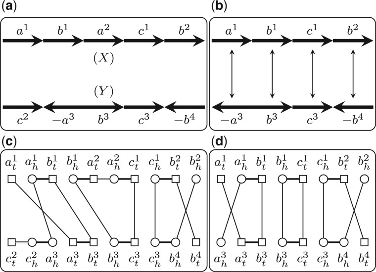
We say consecutive genes on one chromosome form a segment. The length of a segment s is defined as the number of genes in s, denoted by $\left|s\right|$. We say two segments in the same genome are independent if they do not contain the same gene. We say segments $s=(a_1,a_2,···,a_n)$ and $t=(b_1,b_2,···,b_n)$ are homologous if a_i and b_i are homologous and have the same sign for all $1\le i\le n$ or a_i and $b_{n+1-i}$ are homologous and have the opposite sign for all $1\le i\le n$. We say segment s is possibly duplicated, if there exists segment t in the same genome such that s and t are independent and homologous. For a genome X, we use $\mathcal{S}(X)$ to denote the set of all the possibly duplicated segments in X (Fig. 1a). We say a subset $S\subset \mathcal{S}(X)$ is independent if every two segments in S are independent. For an independent subset $S\subset \mathcal{S}(X)$, we use $X\setminus S$ to denote the new genome after removing all genes appearing in the segments in S from X. Given two genomes X and Y, we say two independent subsets $S\subset \mathcal{S}(X)$ and $T\subset \mathcal{S}(Y)$ are consistent if $X\setminus S$ and $Y\setminus T$ have the same gene content, i.e. for each gene family $f\in \mathcal{A}(X)\cup \mathcal{A}(Y)$, we have $|F(X\setminus S,f)|=|F(Y\setminus T,f)|$ (Fig. 1a). In this article, we assume that the given two genomes X and Y satisfy that $\mathcal{A}(X)=\mathcal{A}(Y)$; otherwise we modify them by removing all the genes that are not in $\mathcal{A}(X)\cap \mathcal{A}(Y)$. With this assumption, there always exist two independent subsets $S\in \mathcal{S}(X)$ and $T\in \mathcal{S}(Y)$ that are consistent.

Fig. 1.

(a) Two genomes X and Y. Genes in the same gene family are represented by the same symbol with different superscripts. We have $\mathcal{S}(X)=\{(a^1),(a^2),(b^1),(b^2)\}$ and $\mathcal{S}(Y)=\{(c^2),(b^3),(c^3),(-b^4)\}$ and $S=\{(a^2)\}$ and $T=\{(c^2)\}$ are two consistent subsets. (b) The genomes $X\setminus S$ and $Y\setminus T$ and the bijection B. (c) The adjacency graph w.r.t. $Q=(S,T,B)$. Black edges are represented by long thin lines, while gray edges by short thick lines. Head extremities are represented by circles, while tail extremities by squares. (d) The extended adjacency graph w.r.t. Q, in which internal edges are represented by double lines

Suppose we are given two independent consistent subsets $S\in \mathcal{S}(X)$ and $T\in \mathcal{S}(Y)$. We denote by $\mathcal{B}(X\setminus S,Y\setminus T)$ the set of bijections that map each gene in $X\setminus S$ to a homologous gene in $Y\setminus T$. If $X\setminus S$ and $Y\setminus T$ contain only singletons, i.e. we have $|F(X\setminus S,f)|=|F(Y\setminus T,f)|=1$ for all $f\in \mathcal{A}(X)\cup \mathcal{A}(Y)$, then we have $|\mathcal{B}(X\setminus S,Y\setminus T)|=1$, and the DCJ distance between $X\setminus S$ and $Y\setminus T$ is well defined and can be computed in linear time (Bergeron et al., 2006). Once a bijection $B\in \mathcal{B}(X\setminus S,Y\setminus T)$ is given, we can relabel $X\setminus S$ and $Y\setminus T$ by assigning each pair of genes in B with a distinct gene family and thus results in two new genomes with only singletons. We denote by d(B) the DCJ distance between these two new genomes induced by bijection B.

In this article, we study the following problem: given two genomes X and Y satisfying $\mathcal{A}(X)=\mathcal{A}(Y)$, and a cost function $c(·)$, which maps each segment in $\mathcal{S}(X)\cup \mathcal{S}(Y)$ to a positive value, compute a triple $Q=(S,T,B)$, where $S\subset \mathcal{S}(X)$ and $T\subset \mathcal{S}(Y)$ are two independent consistent subsets and $B\in \mathcal{B}(X\setminus S,Y\setminus T)$, such that the total cost of Q, $\gamma (Q)={\displaystyle {\sum }_{s\in S\cup T}c}(s)+d(B)$, is minimized.

3 ILP formulation

We now formulate the above problem as an integer linear program. To achieve that, we first introduce the adjacency graph in Section 3.1, which is the essential data structure to compute the DCJ distance. We also propose a new extension of the adjacency graph, called the extended adjacency graph, which can incorporate duplicated genes and thus forms the basis for the following ILP formulation. We then describe a capping method to remove the telomeres, in Section 3.2, which allows us only to count the number of cycles when computing the DCJ distance. On the basis of them, we finally give the ILP formulation in Section 3.3.

3.1 Adjacency graph

We first introduce some notations. The two ends of a gene a are called extremities. The head is denoted by a_h and the tail is denoted by a_t. The set of all extremities in genome X is called the extremity set of X, denoted by $\mathcal{E}(X)$. If genes a and b are homologous, we also say the two corresponding extremity pairs, a_h and b_h, a_t and b_t, are homologous. Two consecutive genes a and b form one adjacency, which is represented by a set of two extremities. Thus, each adjacency comes in one of the four types: $\{a_t,b_t\},\{a_h,b_t\}$, $\{a_t,b_h\}$ and $\{a_h,b_h\}$. If gene a lies at one end of a linear chromosome, then this end can be represented by a set of one extremity, $\left\{a_h\right\}$ or $\left\{a_t\right\}$, called a telomere.

Suppose that we are given a triple $Q=(S,T,B)$, where $S\subset \mathcal{S}(X)$, $T\subset \mathcal{S}(Y)$ are two independent consistent subsets and $B\in \mathcal{B}(X\setminus S,Y\setminus T)$. We can build the adjacency graph w.r.t. Q, denoted by G(Q), as follows. We first build $X\setminus S$ and $Y\setminus T$ through removing all genes in $S\cup T$ and take all the extremities in them, i.e. $\mathcal{E}(X\setminus S)\cup \mathcal{E}(Y\setminus T)$, as the vertices of G(Q). Then for each adjacency in $X\setminus S$ and $Y\setminus T$, we add one gray edge to connect the two extremities in it. Finally, for each pair of homologous extremities specified by B (each homologous gene pair in B specifies two pairs of homologous extremities), we add one black edge to connect them (Fig. 1a–c). Clearly, in G(Q), the degree of each vertex is at most 2, and thus it consists of a set of vertex-disjoint cycles and paths. The length of a cycle (or a path) is defined as the number of black edges in it. Let c be the number of cycles and o be the number of odd-length paths in G(Q). We have that the DCJ distance induced by B can then be computed as $d(B)=n-c-o/2$, where n is the number of genes in $X\setminus S$ (Bergeron et al., 2006).

Given a triple $Q=(S,T,B)$ defined above, we propose an equivalent form of G(Q), called the extended adjacency graph w.r.t. Q, denoted by $G\prime (Q)$. The set of vertices of $G\prime (Q)$ includes all the extremities in X and Y, i.e. $\mathcal{E}(X)\cup \mathcal{E}(Y)$. For each adjacency in X and Y, there is one gray edge connecting the two extremities in it. For each pair of homologous extremities specified by B, there is one black edge connecting them. For each gene contained in some segment in $S\cup T$, there is one internal edge connecting the two extremities in this gene (Fig. 1d). The difference between $G\prime (Q)$ and G(Q) is that, the latter one explicitly removes those extremities in the genes in $S\cup T$, whereas the former one keeps them but adds internal edges connecting the two extremities in those genes. Clearly, $G\prime (Q)$ also consists a set of vertex-disjoint cycles and paths, and there is a one-to-one correspondence between the connected components in G(Q) and that in $G\prime (Q)$. Thus, the DCJ distance induced by B can also be computed as $d(B)=n-c\prime -o\prime /2$, where $c\prime$ is the number of cycles and $o\prime$ is the number of odd-length paths in $G\prime (Q)$, and n is the number of genes in $X\setminus S$. As we will see later, this extended adjacency graph is the key point in devising the ILP formulation.

3.2 Add capping genes

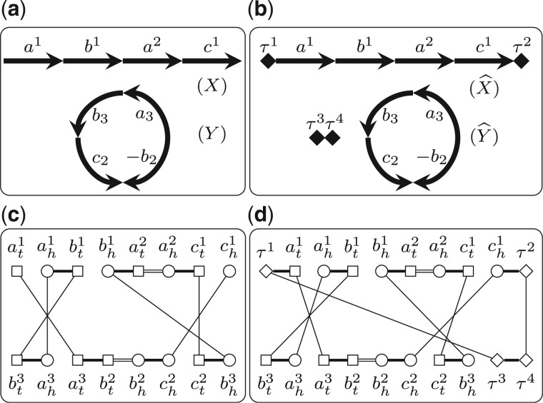
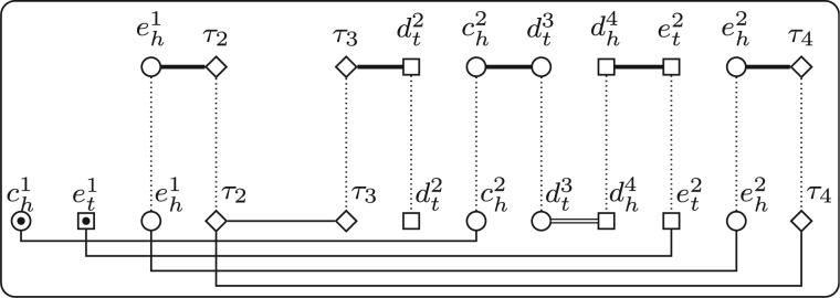
In Shao and Lin (2012), we described a method to remove telomeres by introducing capping genes. A capping gene contains only one extremity, which combines with the adjacent telomere (or another capping gene) to form one adjacency. All capping genes are homologous to each other, forming a distinct gene family, denoted by $f_{\tau }$. Given two genomes X and Y with l_X and l_Y linear chromosomes, respectively (without loss of generality, we assume that $l_X\ge l_Y$), we first add one capping gene to each end of all the linear chromosomes in X and Y; then we add $(l_X-l_Y)$ dummy chromosomes, each of which contains only a pair of capping genes, to genome Y (Fig. 2). We denote by $\widehat{X}$ and $\widehat{Y}$ the two new genomes after adding capping genes for X and Y. Clearly, we have $|F(\widehat{X},f_{\tau })|=|F(\widehat{Y},f_{\tau })|$. Thus, given a pair of independent consistent subsets $S\subset \mathcal{S}(X)$ and $T\subset \mathcal{S}(Y)$, we know that $\widehat{X}\setminus S$ and $\widehat{Y}\setminus T$ also have the same gene content. Using the same argument as in Shao et al.. (2014), we can prove that

$$\underset{\widehat{B}\in \mathcal{B}(\widehat{X}\setminus S,\widehat{Y}\setminus T)}{\min }d(\widehat{B})=\underset{B\in \mathcal{B}(X\setminus S,Y\setminus T)}{\min }d(B),$$

and the optimal B can be recovered from the optimal $\widehat{B}$ through discarding the pairs with capping genes. This statement allows us to add capping genes to remove telomeres on the two given genomes without affecting the optimal bijection. Since the two new genomes $\widehat{X}$ and $\widehat{Y}$ do not contain telomeres, we have that for any triple $Q=(S,T,\widehat{B})$, where $S\subset \mathcal{S}(X)$, $T\subset \mathcal{S}(Y)$ and $\widehat{B}\in \mathcal{B}(\widehat{X}\setminus S,\widehat{Y}\setminus T)$, both G(Q) and $G\prime (Q)$ contain only cycles (Fig. 2). This property allows us only to count the number of cycles when computing the DCJ distance, which simplifies the following ILP formulation.

Fig. 2.

(a) Two genomes X and Y. (b) The genomes $\widehat{X}$ and $\widehat{Y}$ after adding capping genes, where capping genes are represented by diamonds. (c) The extended adjacency graph w.r.t. (S, T, B), where $S=\{(a^2)\},T=\{(b^2)\}$ and B maps a¹, b¹ and c¹ to a³, b³ and c², respectively. (d) The extended adjacency graph w.r.t. $(S,T,\widehat{B})$, where $\widehat{B}$ consists of the two pairs mapping ${\tau }^1$ and ${\tau }^2$ to ${\tau }^3$ and ${\tau }^4$, respectively, and those pairs in B

3.3 ILP formulation

Let X and Y be two given genomes after adding capping genes. Let $Q^{*}=(S^{*},T^{*},B^{*})$ be the optimal triple minimizing ${\displaystyle {\sum }_{s\in S^{*}\cup T^{*}}c}(s)+d(B^{*})$, where we have $S^{*}\subset \mathcal{S}(X),T^{*}\subset \mathcal{S}(Y)$ and $B^{*}\in \mathcal{B}(X\setminus S^{*},Y\setminus T^{*})$. (Notice that here X and Y may contain capping genes, but we define $\mathcal{S}(X)$ and $\mathcal{S}(Y)$ are in terms of the original genomes, which do not contain segments with capping genes.) To facilitate our description, we use $a\in X$ to denote that gene a is contained in genome X. We use $a\in s$ to denote that gene a is contained in segment s. We denote by f_a the gene family to which gene a belongs. We say gene a is duplicated in $Q^{*}$, if there exists one segment $s\in S^{*}\cup T^{*}$ such that $a\in s$ and nonduplicated otherwise.

We now give the ILP formulation to compute $Q^{*}$. For each segment $s\in \mathcal{S}(X)\cup \mathcal{S}(Y)$, we have one binary variable x_s to indicate whether $s\in S^{*}\cup T^{*}$. For each gene $a\in X\cup Y$, we have one binary variable y_a to indicate whether a is duplicated in $Q^{*}$. We use the following two sets of constraints to guarantee that y_a = 1 if and only if there exists one segment $s\in S^{*}\cup T^{*}$ such that $a\in s$:

$$\begin{array}{c}\underset{a}{y}\hspace{1em}\ge \underset{s}{\hspace{1em}x},\forall s\in \mathcal{S}(X)\cup \mathcal{S}(Y)\text{\hspace{0.5em}and\hspace{0.5em}}\forall a\in s;\\ \underset{a}{y}\hspace{1em}\le {\displaystyle \sum _{s\in \mathcal{S}(X)\cup \mathcal{S}(Y):a\in s}}\underset{s}{x},\forall a\in X\cup Y.\end{array}$$

We require that these segments in $S^{*}\cup T^{*}$ are independent, i.e. there do not exist two of them that contain the same gene:

$${\displaystyle \sum _{s\in \mathcal{S}(X)\cup \mathcal{S}(Y):a\in s}\underset{s}{x}}\le 1,\forall a\in X\cup Y.$$

We also require that $X\setminus S^{*}$ and $Y\setminus T^{*}$ have the same gene content, i.e. for each gene family there must be an equal number of nonduplicated genes in $Q^{*}$ in this family in each genome:

$${\displaystyle \sum _{a\in F(X,f)}(1-y_a)}={\displaystyle \sum _{b\in F(Y,f)}(1-y_b)},\forall f\in \mathcal{A}(X).$$

And for each gene family, at least one gene is nonduplicated in $Q^{*}$:

$$\begin{array}{c}{\displaystyle \sum _{a\in F(X,f)}(1-y_a)}\hspace{1em}\ge \hspace{1em}1,\forall f\in \mathcal{A}(X);\\ {\displaystyle \sum _{b\in F(Y,f)}(1-y_b)}\hspace{1em}\ge \hspace{1em}1,\forall f\in \mathcal{A}(Y).\end{array}$$

For each pair of homologous genes $a\in X$ and $b\in Y$, we add one binary variable $\underset{a,b}{z}$ to indicate whether $B^{*}$ contains this pair. We require that for each gene in $X\cup Y$, it is mapped to exactly one homologous gene in the opposite genome if and only if it is nonduplicated in $Q^{*}$:

$$\begin{array}{c}{\displaystyle \sum _{b\in F(Y,f_a)}{z}_{a,b}}=1-y_a,\forall a\in X;\\ {\displaystyle \sum _{a\in F(X,f_b)}{z}_{a,b}}=1-y_b,\forall b\in Y.\end{array}$$

These constraints guarantee that these pairs in $B^{*}$ form a valid bijection between the genes in $X\setminus S^{*}$ and those in $Y\setminus T^{*}$. To compute $d(B^{*})$, we need to count the number of cycles in $G\prime (Q^{*})$. We add a variable l_e for each extremity $e\in \mathcal{E}(X)\cup \mathcal{E}(Y)$ to represent the label of e. We then assign a distinct upper bound for l_e, denoted by U_e (for example, we can just sort all the extremities in $\mathcal{E}(X)\cup \mathcal{E}(Y)$ in an arbitrary order and assign U_e as the index of e in the sorted list):

$$0\le l_e\le U_e,\forall e\in \mathcal{E}(X)\cup \mathcal{E}(Y).$$

We then require that all the extremities in the same cycle in $G\prime (Q^{*})$ have the same label. This can be achieved by forcing that the two extremities connected by any edge in $G\prime (Q^{*})$ have the same label. To guarantee this, we add the following three groups of constraints, each of which corresponds to one type of edges. First, we require that the two extremities in each adjacency have the same label (these constraints correspond to the gray edges):

Second, we require that each pair of extremities specified by $B^{*}$ have the same label (these constraints correspond to the black edges). To achieve that, we add the following four constraints for each pair of homologous genes $a\in X$ and $b\in Y$ (if a and b are capping genes, then we have a_h = a_t and b_h = b_t and thus the following four constraints degenerate into two):

$$\begin{array}{c}\underset{\underset{h}{a}}{l}\le \underset{\underset{h}{b}}{l}+(1-\underset{a,b}{z})·\underset{\underset{h}{a}}{U};\\ \underset{\underset{h}{b}}{l}\le \underset{\underset{h}{a}}{l}+(1-\underset{a,b}{z})·\underset{\underset{h}{b}}{U};\\ \underset{\underset{t}{a}}{l}\le \underset{\underset{h}{b}}{l}+(1-\underset{a,b}{z})·\underset{\underset{t}{a}}{U};\\ \underset{\underset{t}{b}}{l}\le \underset{\underset{h}{a}}{l}+(1-\underset{a,b}{z})·\underset{\underset{t}{b}}{U}.\end{array}$$

Third, we require that the two extremities in each duplicated gene have the same label (these constraints correspond to the internal edges):

$$\begin{array}{c}{l}_{a_h}\le l_{a_t}+(1-y_a)·U_{a_h},\forall a\in X\cup Y;\\ l_{a_t}\le l_{a_h}+(1-y_a)·U_{a_t},\forall a\in X\cup Y.\end{array}$$

We then add a binary variable w_e for extremity e to indicate whether l_e reaches its upper bound:

$$w_e·U_e\hspace{1em}\le \hspace{1em}{l}_e,\forall e\in \mathcal{E}(X)\cup \mathcal{E}(Y).$$

Since all the extremities in the same cycle in $G\prime (Q^{*})$ are forced to have the same label, and all label variables have distinct upper bounds, we know that for each cycle in $G\prime (Q^{*})$ at most one extremity can have its label reaching its upper bound. Thus, we have that

$${\displaystyle \sum _{e\in \mathcal{E}(X)\cup \mathcal{E}(Y)}{w}_e}$$

is exactly the number of cycles in $G\prime (Q^{*})$. And $d(B^{*})$ can then be computed by

$$\left|X\right|-{\displaystyle \sum _{a\in X}{y}_a}-{\displaystyle \sum _{e\in \mathcal{E}(X)\cup \mathcal{E}(Y)}{w}_e},$$

where the first two items give the number of genes in $X\setminus S^{*}$.

Finally, we set the objective function of the ILP as

$$\min {\displaystyle \sum _{s\in \mathcal{S}(X)\cup \mathcal{S}(Y)}c}(s)·x_s+\left|X\right|-{\displaystyle \sum _{a\in X}{y}_a}-{\displaystyle \sum _{e\in \mathcal{E}(X)\cup \mathcal{E}(Y)}{w}_e}.$$

4 Identify optimal substructures

Given two genomes X and Y after adding capping genes, we say two homologous segments s in X and t in Y form a pair of shared segments, denoted by $\langle s,t\rangle$. Intuitively, shared segments are more likely to be nonduplicated and mapped to each other. Below, we give one sufficient condition and one algorithm to decide whether a pair of shared segments is in some optimal solution, i.e. in this optimal solution, a_i and b_i are nonduplicated and a_i is mapped to b_i, for all $1\le i\le n$. From now on, we assume that the cost function only depends on the length of the segments, i.e. we assume that if $\left|s\right|=\left|t\right|$ then we have $c(s)=c(t)$.

4.1 A sufficient condition

We say gene a in genome X is isolated, if there does not exist any segment $s\in \mathcal{S}(X)$ such that $a\in s$ and $\left|s\right|\ge 2$. The following theorem gives a sufficient condition to decide whether a pair of shared segments of length two is an optimal substructure.

Theorem 1 —

Let $p=\langle (a^1,b^1),(a^2,b^2)\rangle$. If we have a¹ and a² are singletons, and b¹ and b² are isolated, then p is in some optimal solution.

Proof —

Let $Q=(S,T,B)$ be an arbitrary triple such that either b¹ or b² is duplicated in Q, or B does not contain $\langle b^1,b^2\rangle$. Below, we will show that we can always build a new triple $Q\prime =(S\prime ,T\prime ,B\prime )$ in which both b¹ and b² are nonduplicated and $B\prime$ contains $\langle b^1,b^2\rangle$ and also verify that $\gamma (Q\prime )\le \gamma (Q)$. Since Q is arbitrary, this proves the theorem.

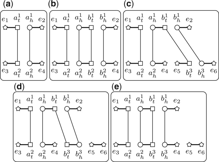
First, assume that in Q both b¹ and b² are duplicated. Let $s\in S$ and $t\in T$ be the segments containing b¹ and b^2, respectively. Since both b¹ and b² are isolated, we know that $\left|s\right|=\left|t\right|=1$. Let $S\prime =S\setminus \left\{s\right\}$ and $T\prime =T\setminus \left\{t\right\}$. We have that $X\setminus S\prime$ and $Y\setminus T\prime$ still have the same content. Let $B\prime =B\cup \{\langle b^1,b^2\rangle \}$. We have that $d(B\prime )=d(B)$, since $X\setminus S\prime$ has one more gene than $X\setminus S$, whereas $G(Q\prime )$ has one more cycle than G(Q) (Fig. 3a and b). Thus, we have $\gamma (Q\prime )={\displaystyle {\sum }_{u\in S\prime \cup T\prime }c}(u)+d(B\prime )={\displaystyle {\sum }_{u\in S\cup T}c}(u)-c(s)-c(t)+d(B)\le {\displaystyle {\sum }_{u\in S\cup T}c}(u)+d(B)=\gamma (Q)$.

Second, assume that in Q gene, b² is duplicated, while b¹ is not (or symmetrically, b¹ is duplicated, while b² is not). Suppose that b¹ is mapped to b³ in B, i.e. $\langle b^1,b^3\rangle \in B$. Let $S\prime =S$ and $T\prime =T\setminus \left\{t\right\}\cup \{t\prime \}$, where $t\in T$ is the segment containing b² and $t\prime$ is the segment containing only gene b³. Clearly, we also have that $X\setminus S\prime$ and $Y\setminus T\prime$ have the same content. Let $B\prime =B\setminus \{\langle b^1,b^3\rangle \}\cup \{\langle b^1,b^2\rangle \}$. To compare $d(B\prime )$ with d(B), consider the difference between $G(Q\prime )$ and G(Q). In fact, we can transform G(Q) into $G(Q\prime )$ through two DCJs on genome Y (after that we need to rename b³ as b²). We first perform one DCJ to cut b³ out to create the adjacency $\{b_h^3,b_t^3\}$ (Fig. 3c and d). This operation might decrease the number of cycles, but the number decreased is at most 1 according to the property of the DCJ model. We then insert b³ back as the neighbor of a² to form the segment $(a^2,b^3)$, which will increase the number of cycles by 1 (Fig. 3d and e). This implies that the number of cycles in $G(Q\prime )$ is no less than that in G(Q). In addition to the fact that $X\setminus S\prime$ and $X\setminus S$ have the same number of genes, we have that $d(B\prime )\le d(B)$. Thus, we have $\gamma (Q\prime )={\displaystyle {\sum }_{u\in S\prime \cup T\prime }c}(u)+d(B\prime )\le {\displaystyle {\sum }_{u\in S\cup T}c}(u)-c(t)+c(t\prime )+d(B)={\displaystyle {\sum }_{u\in S\cup T}c}(u)+d(B)=\gamma (Q)$. The last equality uses the assumption that the cost function only depends on the length of the segments.

Third, assume that in Q both b¹ and b² are nonduplicated, and b¹ is mapped to b³ while b⁴ is mapped b². Let $S\prime =S,T\prime =T$ and $B\prime =B\setminus \{\langle b^1,b^3\rangle ,\langle b^4,b^2\rangle \}\cup \{\langle b^1,b^2\rangle ,\langle b^4,b^3\rangle \}$. Using the same technique in the Theorem 1 (Shao et al., 2014), we can prove that $d(B\prime )\le d(B)$. Thus, we still have $\gamma (Q\prime )={\displaystyle {\sum }_{u\in S\prime \cup T\prime }c}(u)+d(B\prime )\le \gamma (Q).$

Fig. 3.

(a,b) The adjacency graph before and after adding $\langle b^1,b^2\rangle$. (c–e) Transforming G(Q) into $G(Q\prime )$ using two DCJs. Irrelevant extremities are represented by stars

4.2 An algorithm

We say a pair of shared segments $p=\langle (\underset{1}{a},\underset{2}{a},\cdots ,\underset{n}{a}),(\underset{1}{b},\underset{2}{b},\cdots ,\underset{n}{b})\rangle$ between genomes X and Y is half fixed, if b_i is singleton for all $1\le i\le n$ (and thus none of them can be duplicated) and all genes in $F(X,\underset{\underset{i}{a}}{f})$ are isolated for all $1\le i\le n$. Let p be such a pair of half fixed shared segments (PHFSS for short). We use $\mathcal{A}(p)$ to denote all the gene families in p, i.e. $\mathcal{A}(p)=\{f_{a_1},f_{a_2},\cdots ,f_{a_n}\}$. In this section, we propose an algorithm to decide whether a PHFSS is in some optimal solution. Notice that for a PHFSS p, if we further know that in some optimal solution a_k is mapped to b_k for some $1\le k\le n$, then we can immediately conclude that the whole p is in some optimal solution by iteratively applying theorem 3.

Let $Q_{\overline{p}}^{*}=(S,T,B)$ be the triple with smallest total cost among these triples that do not contain p (i.e. b_i is not mapped to a_i for all $1\le i\le n$). We now modify $Q_{\overline{p}}^{*}$ to replace $\underset{i}{a}\prime$ with a_i, where $\underset{i}{a}\prime$ is the gene that are mapped to b_i in $Q_{\overline{p}}^{*}$. Notice that $\{(\underset{1}{a}),(\underset{2}{a}),\cdots ,(\underset{n}{a})\}\subset S$, since a_i is duplicated in $Q_{\overline{p}}^{*}$ (because b_i is singleton and $\underset{i}{a}\prime$ is nonduplicated in $Q_{\overline{p}}^{*}$) and all genes in $F(X,\underset{\underset{i}{a}}{f})$ are isolated. Let $S\prime =S\setminus \{(\underset{1}{a}),\cdots ,(\underset{n}{a})\}\cup$ $\{(\underset{1}{a}\prime ),\cdots ,(\underset{n}{a}\prime )\},B\prime =B\setminus \{\langle \underset{1}{a}\prime ,\underset{1}{b}\rangle ,\cdots ,\langle \underset{n}{a}\prime ,\underset{n}{b}\rangle \}\cup \{\langle \underset{1}{a},\underset{1}{b}\rangle ,\cdots ,$ $\langle \underset{n}{a},\underset{n}{b}\rangle \}$ and $Q_p^{*}=(S\prime ,T,B\prime )$. Clearly $Q_p^{*}$ contains p. According to the definition of $Q_{\overline{p}}^{*}$, if we can show that $\gamma (Q_p^{*})\le \gamma (Q_{\overline{p}}^{*})$, then p is in some optimal solution. From the construction of $Q_p^{*}$, we can see clearly that the cost of the segmental duplications in $Q_{\overline{p}}^{*}$ is equal to that in $Q_p^{*}$. Thus, we only need to compare the number of DCJs between $Q_{\overline{p}}^{*}$ and $Q_p^{*}$.

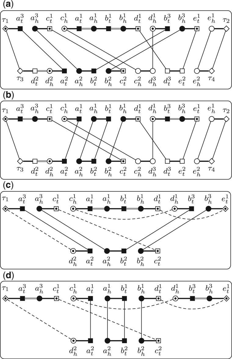
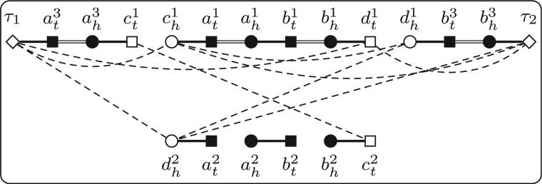
We compare the number of cycles in $G\prime (Q_{\overline{p}}^{*})$ and $G\prime (Q_p^{*})$. Notice that $G\prime (Q_{\overline{p}}^{*})$ and $G\prime (Q_p^{*})$ differ only on these gene families in $\mathcal{A}(p)$. We now define a new graph to focus on $\mathcal{A}(p)$ while hiding others. Let Q be a triple and p be a PHFSS. We can build the reduced adjacency graph w.r.t. Q and p, denoted by R(Q, p), as follows. The vertices of R(Q, p) are divided into two types, the core vertices, which are exactly those extremities in the genes in the gene families in $\mathcal{A}(p)$ and the boundary vertices, which consist of these extremities that form adjacencies with core vertices (Fig. 4a and b). The edges of R(Q, p) are divided into four types, gray edges, black edges, internal edges and reduced edges. For any two vertices in R(Q, p), they are connected by gray edges or internal edges, if and only if they are connected by the same type of edge in $G\prime (Q)$. For any two core vertices in R(Q, p), they are connected by one black edge if and only if they are connected by one black edge in $G\prime (Q)$. For any two boundary vertices in R(Q, p), they are connected by one reduced edge if there exists one path connecting them in $G\prime (Q)$ without going through any core vertices or boundary vertices (except its two ends). Clearly, R(Q, p) also consists of a set of vertex-disjoint cycles (Fig. 4c and d).

Fig. 4.

$X=(a^3,c^1,a^1,b^1,d^1,b^3,e^1),Y=(d^2,a^2,b^2,c^2,-d^3,e^2)$. $p=\langle (a^1,b^1),(a^2,b^2)\rangle$. The four subgraphs show $G\prime (Q_{\overline{p}}^{*}),G\prime (Q_p^{*}),R(Q_{\overline{p}}^{*},p)$ and $R(Q_p^{*},p)$, respectively. The core vertices are shown as solid patterns, and the boundary vertices are shown as patterns with one inner point. Reduced edges are shown as dashed lines

We claim that the difference of the number of cycles between $G\prime (Q_{\overline{p}}^{*})$ and $G\prime (Q_p^{*})$ is the same as that between $R(Q_{\overline{p}}^{*},p)$ and $R(Q_p^{*},p)$. In fact, the cycles that do not contain any core vertices or boundary vertices are the same between $Q_{\overline{p}}^{*}$ and $Q_p^{*}$ according to the construction of $Q_p^{*}$ and those cycles do not appear in either $R(Q_{\overline{p}}^{*},p)$ or $R(Q_p^{*},p)$. Moreover, for each cycle in $G\prime (Q_{\overline{p}}^{*})$ that contains some core vertices, there exists one corresponding cycle in $R(Q_{\overline{p}}^{*},p)$, since the reduction procedure in constructing $R(Q_{\overline{p}}^{*},p)$ can only shorten the length of each cycle, while it cannot merge or split it. It is the same for $G\prime (Q_p^{*})$ and $R(Q_p^{*},p)$. Thus, the claim holds. Furthermore, the reasoning used here also implies that we can construct $R(Q_p^{*},p)$ directly from $R(Q_{\overline{p}}^{*},p)$, rather than from $G\prime (Q_p^{*})$: we can first replace the black edges corresponding to $\langle \underset{i}{a}\prime ,\underset{i}{b}\rangle$ with that corresponding to $\langle \underset{i}{a},\underset{i}{b}\rangle$ and then replace the internal edges corresponding to a_i with that corresponding to $\underset{i}{a}\prime$.

In summary, once we know $R(Q_{\overline{p}}^{*},p)$, we can then construct $R(Q_p^{*},p)$ and compare the number of cycles in them. If the number of cycles in $R(Q_p^{*},p)$ is no less than that in $R(Q_{\overline{p}}^{*},p)$, then p is in some optimal solution. However, the problem is that we do not know $R(Q_{\overline{p}}^{*},p)$. Our strategy is to enumerate all the possibilities of $R(Q_{\overline{p}}^{*},p)$. The vertices of $R(Q_{\overline{p}}^{*},p)$, i.e. all the core vertices and all the boundary vertices w.r.t. p, can be computed in advance very easily. All the genes of a_i, $1\le i\le n$, are duplicated in $R(Q_{\overline{p}}^{*},p)$ by definition, and thus the two extremities in a_i are always connected by one internal edge in $R(Q_{\overline{p}}^{*},p)$. All genes in $F(X,f_{a_i})\setminus \left\{a_i\right\}$ are possibly mapped to b_i in $R(Q_{\overline{p}}^{*},p)$. For any two boundary vertices (maybe in the same genome), we need to check whether they can be connected by one reduced edge in $R(Q_{\overline{p}}^{*},p)$, i.e. whether there exists one possible path connecting them that does not go through any other core vertices or boundary vertices. Notice that this path must be alternating, i.e. the edges with odd indices must be either black edges or internal edges and the edges with even indices must be gray edges (Fig. 4c and d).

There exists a linear time algorithm to decide the existence of an alternating path between two given vertices (Bang-Jensen and Gutin, 1998). We now adapt it for our use. Given a PHFSS p and two boundary vertices x and y, the algorithm first build a graph with $\underset{1}{V}\cup \underset{2}{V}\cup \{x,y\}$ as its vertices, where V₁ is the set of all extremities except all the core vertices and boundary vertices and V₂ is a copy of V₁. Two extremities in V₁ are connected by one gray edge if they form one adjacency. Two homologous extremities in V₂ in different genomes are connected by one black edge, and the two extremities in V₂ in a possibly duplicated gene are connected by one internal edge. We connect x (resp. y) to its all homologous extremities in V₂ in the opposite genome by black edges. Finally, all the counterparts between V₁ and V₂ are connected by bridging edges (Fig. 5). Clearly, all the bridging edges form a matching of size $\left|\underset{1}{V}\right|$, denoted by M. The algorithm then computes an augmenting path w.r.t. M using the Blossom algorithm, which takes linear time. We claim that such an augmenting path exists if and only if there exists one alternating path connecting x and y without going through any core vertices or boundary vertices. In fact, if such an augmenting path exists, then the two ends of this path must be x and y, since they are the only two unmatched vertices. We claim that the edges in the augmenting path that are not in M form an alternating path connecting x and y. This is because edges in M are spanning V₁ and V₂, whereas gray edges are all inside in V₁ and black edges and internal edges are inside in V₂. The opposite side of statement can be reasoned in a similar way.

Fig. 5.

The underlying graph used to decide the existence of an alternating path connecting $c_h^1$ and $e_t^1$ w.r.t. p for the same instance in Figure 4. All bridging edges are shown as dotted lines

The algorithm to decide whether a given PHFSS p is in some optimal solution proceeds as follows. The first phase of the algorithm is to compute the core vertices and the boundary vertices w.r.t. p and then for each pair of boundary vertices, to check whether they can be connected by a reduced edge. If the total number of edges (reduced edges plus those among core vertices) is larger than $\log n$, the algorithm terminates. Otherwise, the algorithm comes to the second phase. It enumerates all the possibilities of $R(Q_{\overline{p}}^{*},p)$: for each possible valid combination of the reduced edges (i.e. they form a matching that covers all the boundary vertices), it enumerates all the possible valid mappings for the genes in $\mathcal{A}(p)$ (a_i cannot be mapped to b_i by the definition of $R(Q_{\overline{p}}^{*},p)$) and the mapping that yields the maximum number of cycles, plus the current combination of the reduced edges, forms one possibility of $R(Q_{\overline{p}}^{*},p)$. After that, for each possibility of $R(Q_{\overline{p}}^{*},p)$, it then builds $R(Q_p^{*},p)$ and compares the number of cycles between them. If the number of cycles in $R(Q_p^{*},p)$ is always no less than that in $R(Q_{\overline{p}}^{*},p)$ for all the possibilities, then the algorithm concludes that p is in some optimal solution.

The above algorithm runs in polynomial time. In fact, the first phase runs in polynomial-time, since we can decide the existence of a reduced edge for each pair of boundary vertices in linear time. In the second phase, the number of edges is in logarithmic-size, which implies that the number of possibilities of $R(Q_{\overline{p}}^{*},p)$ is in polynomial size. Thus, the second phase also runs in polynomial time.

We remark that usually not all pairs of boundary vertices can be connected by a reduced edge (Fig. 6). In fact, if this is not the case, then there always exists one possibility such that $R(Q_{\overline{p}}^{*},p)$ contains more cycles than $R(Q_p^{*},p)$, in which case the algorithm fails. In other words, the first phase to identify possible reduced edges is very essential, which not only decreases the number of possibilities but more importantly makes the algorithm capable of identifying optimal substructures. We also remark that this algorithm is a sufficient test, i.e. if it returns ‘yes’, then p is guaranteed in some optimal solution. However, if it returns ‘no’, then it is still possible that p is in some optimal solution. This is because two reduced edges in $R(Q_{\overline{p}}^{*},p)$ might not be able to coexist in $G\prime (Q_{\overline{p}}^{*})$.

Fig. 6.

All the possible reduced edges in $R(Q_{\overline{p}}^{*},p)$ for the same instance in Figure 4. We can verify that among all possibilities of $R(Q_{\overline{p}}^{*},p)$, the number of cycles in $R(Q_p^{*},p)$ is always no less than that in $R(Q_{\overline{p}}^{*},p)$. Thus, in this instance, p is optimal

We can apply the theorem in Section 4.1 and the algorithm in Section 4.2 on all shared segments to verify their optimality. If such an optimal substructure is identified, we immediately fix it and update the genomes through assigning each pair of genes in it a distinct gene family. We can iteratively repeat this process until no such optimal substructure can be found. This serves as a preprocessing algorithm to simplify the problem before calling the ILP solver. The performance of this preprocessing algorithm on real genomes is analyzed in Table 4.

Table 4.

Composition of B

Species pairs	Trivial (%)	Predetermined (%)	Remaining (%)	$\left|B\right|$
G.g. and H.s.	51.5	47.9	0.5	16 213
G.g. and M.m.	48.7	49.5	1.6	15 015
G.g. and P.a.	50.7	48.5	0.7	15 271
G.g. and R.n.	46.3	50.5	3.0	14 983
H.s. and M.m.	51.0	47.5	1.3	15 572
H.s. and P.a.	52.3	47.1	0.4	15 481
H.s. and R.n.	48.5	49.5	1.8	15 379
M.m. and P.a.	50.0	48.6	1.2	14 620
M.m. and R.n.	48.9	49.4	1.6	16 347
R.n. and P.a.	47.7	50.1	2.0	14 534

5 Set the cost

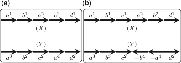
Under a parsimonious model, it is natural to set a unit cost for all segmental duplications (as we do for all DCJs). However, in this case, two segmental duplications, one in each genome, that create a pair of shared segments can be always explained as two DCJs with the same total cost. Consider the example in Figure 7a, for which we have two optimal solutions with total cost of 2: one is to regard a² and a⁴ as duplicated genes, and the other uses two DCJs, which first cut a² out from X and then insert it back between c¹ and d¹. The scenario in the second case (two DCJs using one circular chromosome as intermediate) requires three inversions to explain, and therefore it is much less unlikely to happen comparing with the first scenario. Thus, to avoid the second case we set $c(·)<1$.

Fig. 7.

(a) An example in which there are two optimal solutions if $c(·)=1$. (b) An example in which there are two optimal solutions if $c(·)=0.5$

On the other hand, if we have $c(·)\le 0.5$, then every DCJ that inverts a possibly duplicated segment can be always explained by two segmental duplications with the same or even better total cost. Consider the example in Figure 7b, for which one solution is to use only one DCJ to invert the segment $(a^2,b^2)$ on X. However, if we have $c(·)\le 0.5$, then we can regard $(a^2,b^2)$ and $(-b^4,-a^4)$ as duplicated segments, whose total cost is at most 1. Thus, to avoid the second case, we need to set $c(·)>0.5$.

Combining the above two facts, in the following experiments, we set $c(·)=0.75$.

6 Infer in-paralogs and orthologs

Under a most parsimonious evolutionary scenario, the duplicated genes in the optimal triple infer the in-paralogs in each genome, whereas the bijection between the nonduplicated genes in the two genomes infers a subset of the orthology pairs [more specifically, positional orthologs (Dewey, 2011)]. In the following, we apply our method to infer in-paralogs and orthologs on both simulated datasets and biological datasets and compare its performance with MSOAR.

6.1 Results on simulated datasets

We simulate a pair of genomes as follows. We start from an ancestor genome with only one linear chromosome consisting of N = 5000 singletons (we also test N = 1000 and N = 2000; the results are not presented since they agree with N = 5000). We then perform S₁ segmental duplications on the ancestor genome to make some gene families contain more than one copy. A segmental duplication randomly chooses a segment of length L and inserts its copy to another random position. The two extant genomes then speciate independently from this ancestor genome. The speciation process on each branch includes randomly mixed S₂ segmental duplications and D DCJs. A DCJ randomly chooses two positions in the genome and then reverses the segment in between. We make sure that the expected number of genes per gene family in each extant genome is 1.5 (this number is comparable to that in human genome, which is 1.46), therefore we have that $\underset{1}{S}+\underset{2}{S}=0.5·N/L$. We further fix $\underset{1}{S}=0.2·N/L$ and $\underset{2}{S}=0.3·N/L$ (we also test $\underset{1}{S}=0$ and $\underset{2}{S}=0.5·N/L$, and the results are almost the same). Thus, a simulation configuration is determined by parameters L and D.

For each pair of simulated genomes X and Y, we take them as input to run MSOAR and our method. For MSOAR, we run its binary version downloaded from http://msoar.cs.ucr.edu/. For our method, we first apply the preprocessing algorithm described in Section 4 and then formulate the simplified problem as an ILP instance, which is solved using the GUROBI solver. We set the time limit to 2 h for each instance, i.e. if the ILP solver does not return the optimal solution in 2 h, we terminate it and return the current sub-optimal solution.

Both methods return triples (S, T, B), where S and T infers the in-paralogs in the two extant genomes, respectively, and B infers the orthology pairs. We now give the measures to evaluate them. First, we regard the problem to infer in-paralogs as a standard binary classification problem: those genes that are generated by segmental duplications in the speciation process are considered as gold standard positive in-paralogs and those genes that are in the segments in $S\cup T$ are considered as predicted positive in-paralogs. Thus, we use the sensitivity and specificity to measure (S, T). To evaluate the performance of B, we refer to those gene pairs in the two extant genomes that correspond to the same gene in the ancestor genome as the true orthology pairs. We therefore use the following way to evaluate B: we say a pair in B is assessable, if at least one of its two genes can be found in some true orthology pair, and the accuracy of B is then defined as the ratio between the number of true orthology pairs in B and the number of assessable pairs in B.

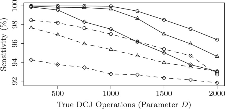
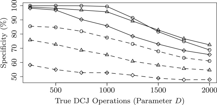
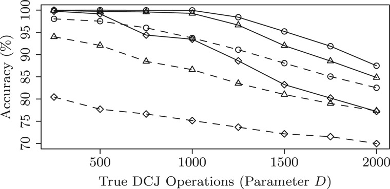
For each parameter configuration, we simulate 10 instances and compute the average sensitivity, specificity and accuracy for both methods. The performance of the two methods is shown in Figures 8–10, where the parameters $L\in \{1,2,5\}$ and D ranges from 250 to 2000. First, we can observe that both methods get very high sensitivity (above 90% on all configurations). However, MSOAR gets relatively low specificity. One reason for this is that MSOAR uses unit cost for both rearrangements and single-gene duplications. According to the discussion in Section 5, unit cost for all operations might misclassify in-paralogs. Second, as D increases, the performance of both methods decreases. This is because the number of DCJs is highly positively correlated to the difficulty of the problem. When $D\le 500$, i.e. roughly 10% of the size of the simulated genome (which is usually the case for real genomes, see Table 2 columns d(B) for some examples), we can see that our method almost gets perfect performance. Third, observe that MSOAR is very sensitive to L even when D is very small. This might be because the evolutionary model for in-paralogs in MSOAR is single-gene duplication, which creates trouble when genomes contain long segmental duplications. Finally, our method outperforms MSOAR on all the configurations.

Fig. 8.

Sensitivity of the inferred in-paralogs. The solid lines and dashed lines track our method and MSOAR, respectively. The circles, triangles and diamonds track L = 1, L = 2 and L = 5, respectively

Fig. 9.

Specificity of the inferred in-paralogs

Fig. 10.

Accuracy of the inferred orthologs

Table 2.

Comparison with MSOAR on inferred operations and total score

Species pairs	$\left|S\right|+\left|T\right|$		d(B)		Total cost
	MSOAR	ILP	MSOAR	ILP	MSOAR	ILP
G.g. and H.s.	1738	1962	670	361	1973.50	1832.50
G.g. and M.m.	2183	2369	1214	891	2851.25	2667.75
G.g. and P.a.	1985	2259	896	530	2384.75	2224.25
G.g. and R.n.	3389	3620	1969	1394	4510.75	4109.00
H.s. and M.m.	1320	1381	909	743	1899.00	1778.75
H.s. and P.a.	1336	1444	497	306	1499.00	1389.00
H.s. and R.n.	2897	2885	1366	1069	3538.75	3232.75
M.m. and P.a.	1731	1825	906	707	2204.25	2075.75
M.m. and R.n.	2621	2739	1176	763	3141.75	2817.25
R.n. and P.a.	3109	3208	1535	1101	3866.75	3507.00

6.2 Results on biological datasets

We compare both methods on five mammalian species, human (H.s.), gorilla (G.g.), orangutan (P.a.), mouse (M.m.) and rat (R.n.). For each species, we collect all the protein-coding genes and download their positions on the chromosomes and the Ensembl gene family names from Ensembl (http://www.ensembl.org). Two genes are considered as homologous if they have the same Ensembl gene family name. Since the tandemly arrayed genes (TAGs) have a different evolutionary model from segmental duplications, we merge each group of TAGs into only one gene through only keeping the first gene in the group while removing all the following ones.

We do the pairwise comparison for all five species, and for each pair of species, we run both methods to obtain triples (S, T, B). We use the same accuracy defined in Section 6.1 to evaluate B. To compute the accuracy, we use the gene symbols (HGNC symbols for primate genes, MGI symbols for mouse genes and RGD symbols for rat genes, downloaded from Ensembl) to define true orthology pairs: those gene pairs that have the same gene symbol form the set of true orthology pairs for each pair of species. We do not have annotation data to serve as gold standard positive in-paralogs (we cannot just regard those genes that are not in the true orthology pairs as gold standard positive in-paralogs, since many genes have not yet been assigned a valid gene symbol). Thus, we are not able to compute the sensitivity and specificity of (S, T).

The comparison on accuracy is shown in Table 1. We can observe that both methods have very high accuracy, indicating that the inferred orthology pairs from gene order data mostly agree with the annotations. On the other hand, our method gets higher accuracy than MSOAR on all the 10 pairs. The running time of MSOAR is also shown in Table 1. On average, for each instance, MSOAR takes 108 min, which is on the same level with our method (120 min for each instance).

Table 1.

Comparison with MSOAR on accuracy

Species pairs	Assessable		Accuracy		Time
	MSOAR	ILP	MSOAR (%)	ILP (%)
G.g. and H.s.	14 898	14 807	98.9	99.1	43
G.g. and M.m.	12 946	12 923	98.7	99.0	100
G.g. and P.a.	11 308	11 262	98.7	99.0	71
G.g. and R.n.	10 831	10 779	97.2	98.0	292
H.s. and M.m.	14 030	13 989	99.1	99.3	61
H.s. and P.a.	12 004	11 955	99.1	99.3	32
H.s. and R.n.	11 748	11 685	97.5	98.1	127
M.m. and P.a.	10 574	10 537	98.9	99.3	68
M.m. and R.n.	12 332	12 280	97.7	98.2	130
R.n. and P.a.	8788	8745	97.6	98.2	157

Bold values highlight larger accuracy. The last column shows the running time of MSOAR (in min).

In Table 2, we compare the number of operations and total score inferred by the two methods to evaluate their ability as an optimizer. First, we can see that our method gets more segmental duplications and many fewer DCJs than MSOAR. One reason for this is that we use smaller weight for segmental duplications. Second, our method gets smaller total cost on all the 10 pairs. This shows the advantage of our exact algorithm over the heuristic applied in MSOAR. Notice that the total cost shown in Table 2 is computed using our weight, i.e. $d(B)+0.75·(|S|+|T|)$, for both methods. However, if the total cost is computed using MSOAR’s weight, i.e. $d(B)+\left|S\right|+\left|T\right|$, our method still has less total cost on all pairs.

In Table 3, we analyze the distribution of the length of the inferred duplicated segments by our method. We can see that most of them are single-gene duplications. We can also observe that the rat genome contains more duplications than the other four genomes.

Table 3.

Distribution of the length of the segments in S and T

Species pairs	S1	S2	$S_{\ge 3}$	$\left|S\right|$	T1	T2	$T_{\ge 3}$	$\left|T\right|$
G.g. and H.s.	98.7	1.2	0.0	1347	95.2	4.3	0.3	615
G.g. and M.m.	98.5	1.3	0.1	1421	96.7	2.9	0.3	948
G.g. and P.a.	97.9	1.8	0.1	1579	98.8	1.1	0.0	680
G.g. and R.n.	98.1	1.6	0.2	1377	94.9	3.7	1.2	2243
H.s. and M.m.	94.8	4.9	0.1	563	96.2	3.5	0.2	818
H.s. and P.a.	93.9	4.8	1.2	807	99.3	0.4	0.1	637
H.s. and R.n.	94.9	4.2	0.7	631	95.3	3.2	1.3	2254
M.m. and P.a.	96.0	3.3	0.6	1109	99.1	0.5	0.2	716
M.m. and R.n.	95.5	3.5	0.9	648	94.5	3.5	1.8	2091
R.n. and P.a.	95.2	3.5	1.2	2472	99.0	0.6	0.2	736

S_k (respectively, T_k) contains the percentage of the segments of length k in S (respectively, T).

In Table 4, we analyze the composition of B returned by our method. If a gene family is a singleton in both genomes, then this pair of genes cannot be duplicated and must be mapped to each other by definition. We call such pair a trivial pair. Observe that roughly half of the pairs in B are trivial pairs (trivial column). We also show the percentage of the pairs that are fixed through the preprocessing algorithm (predetermined column). We can see that this preprocessing algorithm is very efficient, which can fix almost all the nontrivial pairs, leaving a very small portion (remaining column) that are to be determined by the ILP. This is because these species contain many shared segments and many isolated genes (because most of the segmental duplications are single-gene duplications), and thus there are many optimal substructures that can be identified by our algorithm.

7 Conclusion and discussion

We proposed an exact algorithm to compute a set of DCJs and segmental duplications with minimum total cost between two given genomes. As far as we know, this is the first exact algorithm to compare two genomes in the presence of duplicated genes with both rearrangements and content-modifying events. This algorithm can be applied to infer in-paralogs and orthologs, and the inferred results were showed highly agreeing with the annotations.

The algorithm described in Section 4.2 has potential to extend. For example, it can be directly used to test whether a general substructure, rather than a single PHFSS, is optimal. Moreover, we made a strong assumption that all genes in the related gene families are isolated, which immediately makes the cost of the segmental duplications trivial to compare and thus allows us to focus on the number of cycles. In fact, we can relax this assumption, as long as we can guarantee that the segmental duplications induced by the substructure that is tested is optimal.

Although the evolutionary model used in our algorithm, i.e. DCJ plus segmental duplication, is already quite general, there are some other events, like tandem duplications, that cannot be explained by this model. We will extend our algorithm for more general models in the future.

Conflict of Interest: none declared.

References

- Bader D., et al. (2001) A fast linear-time algorithm for inversion distance with an experimental comparison. J. Comput. Biol., 8, 483–491. [DOI] [PubMed] [Google Scholar]
- Bang-Jensen J., Gutin G. (1998) Alternating cycles and trails in 2-edge-coloured complete multigraphs. Discrete Math. , 188, 61–72. [Google Scholar]
- Bergeron A., et al. (2006) A unifying view of genome rearrangements. In: Proceedings of the 6th Workshop on Algorithms in Bioinformatics (WABI’06), Volume 4175 of Lecture Notes in Computer Science Springer Verlag, Berlin, pp. 163–173. [Google Scholar]
- Bergeron A., et al. (2009) A new linear-time algorithm to compute the genomic distance via the double cut and join distance. Theor. Comput. Sci., 410, 5300–5316. [Google Scholar]
- Braga M., et al. (2010) Genomic distance with DCJ and indels. In: Proceedings of the 10th Workshop on Algorithms in Bioinformatics (WABI’10), Volume 6293 of Lecture Notes in Computer Science. Springer Verlag, Berlin, pp. 90–101. [Google Scholar]
- Braga M., et al. (2011) Double cut and join with insertions and deletions. J. Comput. Biol. , 18, 1167–1184. [DOI] [PubMed] [Google Scholar]
- Chen X. (2010) On sorting permutations by double-cut-and-joins. In: Proceedings of the 16th Conference On Computing and Combinatorics (COCOON’10), volume 6196 of Lecture Notes in Computer Science. Springer Verlag, Berlin, pp. 439–448. [Google Scholar]
- Chen X., et al. (2005) Assignment of orthologous genes via genome rearrangement. ACM/IEEE Trans. Comput. Biol. Bioinform., 2, 302–315. [DOI] [PubMed] [Google Scholar]
- Dewey C. (2011) Positional orthology: putting genomic evolutionary relationships into context. Brief. Bioinform. , 12, 401–412. [DOI] [PMC free article] [PubMed] [Google Scholar]
- El-Mabrouk N. (2001) Sorting signed permutations by reversals and insertions/deletions of contiguous segments. J. Discrete Algorithms , 1, 105–122. [Google Scholar]
- Fu Z., et al. (2007) MSOAR: a high-throughput ortholog assignment system based on genome rearrangement. J. Comput. Biol. , 14, 1160–1175. [DOI] [PubMed] [Google Scholar]
- Gu W., et al. (2008) Mechanisms for human genomic rearrangements. Pathogenetics , 1, 4. [DOI] [PMC free article] [PubMed] [Google Scholar]
- Hannenhalli S., Pevzner P. (1995) Transforming cabbage into turnip (polynomial algorithm for sorting signed permutations by reversals). In: Proceedings of the 27th Annual ACM Symposium Theory of Computing (STOC’95). ACM Press, New York, pp. 178–189. [Google Scholar]
- Holloway P., et al. (2013) Ancestral genome organization: an alignment approach. J. Comput. Biol. , 20, 280–295. [DOI] [PubMed] [Google Scholar]
- Kahn C., Raphael B. (2008) Analysis of segmental duplications via duplication distance. Bioinformatics , 24, i133–i138. [DOI] [PubMed] [Google Scholar]
- Kahn C., et al. (2010) Parsimony and likelihood reconstruction of human segmental duplications. Bioinformatics , 26, i446–i452. [DOI] [PMC free article] [PubMed] [Google Scholar]
- Moret B., et al. (2013) Rearrangements in phylogenetic inference: compare, model, or encode? In: Chauve C., et al. (eds.) Models and Algorithms for Genome Evolution, Volume 19 of Computational Biology. Springer Verlag, Berlin, pp. 147–172. [Google Scholar]
- Shao M., Lin Y. (2012) Approximating the edit distance for genomes with duplicate genes under DCJ, insertion and deletion. BMC Bioinformatics , 13(Suppl 19), S13. [Google Scholar]
- Shao M., et al. (2014) An exact algorithm to compute the DCJ distance for genomes with duplicate genes. In: Proceedings of the 18th International Conference on Computations of Molecular Biology (RECOMB’14), Volume 8394 of Lecture Notes in Computer Science. Springer Verlag, Berlin, pp. 280–292. [Google Scholar]
- Yancopoulos S., et al. (2005) Efficient sorting of genomic permutations by translocation, inversion and block interchange. Bioinformatics , 21, 3340–3346. [DOI] [PubMed] [Google Scholar]