

Abstract
The temporal generalization gradient produced by the peak-interval (PI) procedure reflects behavior under the control of positive reinforcement for responding after the criterial time, but shows negligible discouragement for early responses. The lack of consequences for premature responding may affect estimates of timing accuracy and precision in the PI procedure. In two experiments, we sought to encourage more accurate timing in pigeons by establishing an opportunity cost for such responding. Concurrent ratio and interval schedules of reinforcement reduced the dispersion of keypecking around the target time. A sequence of three response-rate states (low-high-low) characterized performance in individual trials. Opportunity cost substantially reduced the mean and standard deviation of the duration of the middle-high state that typically enveloped the target time, indicating improved temporal acuity. We suggest a model as a first-order approximation to timing with opportunity cost.
In the peak-interval (PI) procedure (Catania, 1970; Roberts, 1981), repeated presentations of a fixed-interval (FI) schedule of reinforcement (Ferster & Skinner, 1957) are interspersed with unsignaled extinction (EXT) trials, known as probe trials. In FI trials, the first response after a criterial time since the onset of a stimulus is reinforced. With enough training, probe trials typically induce a peak in response rate around the time at which the reinforcer is delivered in FI trials. Many studies use the PI procedure as a measure of an organism's ability to time intervals (Gibbon & Church, 1990). Studies have employed the PI procedure in studying timing in humans (Rakitin et al., 1998), rats (e.g., Yi, 2007), fish (Drew, Zupan, Cooke, Couvillon, & Balsam, 2005), and several species of birds (e.g., Brodbeck, Hampton, & Cheng, 1998; P. E. Taylor, Haskell, Appleby, & Waran, 2002). Various quantitative models have been formulated to describe PI performance (Gallistel & Gibbon, 2000; Killeen & Fetterman, 1988; Killeen & Taylor, 2000; Kirkpatrick, 2002; Machado, 1997), and significant advances in the neurobiology and pharmacology of timing rest on evidence produced using the PI procedure (Asgari et al., 2006; R.-K. Cheng, Ali, & Meck, 2007; Gooch, Wiener, Portugal, & Matell, 2007; Meck, 2006; Sandstrom, 2007; K. M. Taylor, Horvitz, & Balsam, 2007). For these endeavors, it is critical to identify the variables that contribute to response rate functions in the PI procedure. In this article, we introduce a variable that has been largely neglected: the opportunity cost of PI timing—that is, the cost of not engaging in other activities while producing the target response.
Our principal motivation for examining the opportunity cost of timing derives from the loose control that FI schedules exert over PI performance. Control is never so tight that animals would respond only at the criterial time, but never so loose that animals would respond at a constant rate throughout PI trials. Could the value of FI reinforcers modulate this control and encourage better timing? It has been shown that the absolute value of reinforcers may affect temporal generalization gradients (Belke & Christie-Fougere, 2006; Ludvig, Conover, & Shizgal, 2007; Plowright, Church, Behnke, & Silverman, 2000). Here, we are concerned with the relative value of FI reinforcers.
A long tradition of research on concurrent schedules of reinforcement has demonstrated that production of a behavior depends not only on reinforcement of that behavior, but also on reinforcement of alternative behaviors (Davison & McCarthy, 1988). Without alternative sources of reinforcement, there is no discouragement for pigeons to respond early in the PI procedure: It would be to the animal's advantage to respond at a constant rate. Timing would then be imprecise, even though the cause is motivational, rather than computational. Animals seldom respond continuously in PI trials, either because they are under the inhibitory control of the prior reinforcer or because such responding would prevent them from collecting other reinforcers, such as those available from interim responses, which may include area-restricted search, adjunctive responses, and simple leisure. These unscheduled sources of reinforcement must play some role in shaping the gradients. In an attempt to bring alternative sources of reinforcement under experimental control, we used concurrent schedules of reinforcement to engender behavior inconsistent with the FI response.
In this study, we analyzed when pigeons started and stopped keypecking in probe PI trials with and without concurrent schedules of reinforcement. Timing statistics that were based on start and stop times allowed us to infer two measures of temporal acuity: accuracy (how close start and stop times were to a criterial time) and precision (how consistent start and stop times and other derived measures are over trials). On the basis of the effects of opportunity cost on these measures, we suggest how to incorporate opportunity cost into models of timing.
Experiment 1
Peak Timing With Concurrent Ratio Schedules
In Experiment 1, pigeons were exposed to concurrent FI, random ratio (RR) schedules of reinforcement. The probability of reinforcement for FI responses changed from 0 to 1 at 15 sec after trial onset. The probability of reinforcement for RR responses was constant. Thus, every time the pigeon pecked on the FI key, it forwent the opportunity for a possible reinforcement from the RR schedule.
Method
Subjects
Six adult homing pigeons (Columba livia) served as subjects. All pigeons had an experimental history of behavioral procedures lasting approximately 1 year. The pigeons were housed individually in a room with a 12:12-h day:night cycle, with dawn at 6:00 a.m. They had free access to water and grit in their home cages. The birds were weighed immediately prior to an experimental session and were excluded from a session if their weight exceeded 8% of running weight (80% of ad lib). When required, supplementary feeding of ACE-HI pigeon pellets (Star Milling Co.) was given at the end of each day, no less than 12 h before experimental sessions were conducted. Supplementary feeding amounts were based on the average of the current deficit and a moving average of amounts fed over the last 15 sessions.
Apparatus
Experimental sessions were conducted in five Med Associates modular test chambers (305 mm long × 241 mm wide × 292 mm high), each enclosed in a sound- and light-attenuating box equipped with a ventilating fan. The front wall, rear walls, and ceiling of the experimental chambers were made of clear plastic. The front wall was hinged and functioned as a door to the chamber. The two side panels were aluminum. The floor consisted of thin metal bars positioned above a drip pan. Three plastic, translucent response keys, 25 mm in diameter, were arranged horizontally on a test panel that formed one side of the chamber. The response keys were located equidistantly 52 mm from the center key, 70 mm below the ceiling, and 26 mm from the nearest wall. The keys could be illuminated by white, green, or red light emitted from two of six diodes mounted behind them. A 77-mm square opening located 20 mm above the floor on the test panel provided access to milo grain when a hopper behind the panel was activated (Coulbourn Instruments, H14-10R). A houselight was mounted 12 mm from the ceiling, on the sidewall opposite the test panel. The ventilation fan mounted on the rear wall of the sound-attenuating chamber provided masking noise of 60 dB. Experimental events were recorded and arranged via a MED-PC interface connected to a PC controlled by MED-PC IV software.
Procedure
General conditions
All pretraining and experimental sessions were conducted daily, generally 7 days a week. Each session consisted of a sequence of trials. Each trial was preceded by a 15-sec intertrial interval (ITI) and was usually terminated by a reinforcer, a 2-sec activation of the hopper. The houselight was on during ITIs and off during experimental trials. Each session ended after 2 h or 120 reinforcer deliveries, whichever happened first. Pretraining and experimental conditions are described in more detail below. The order of presentation and number of sessions in each condition are listed in Table 1.
Table 1. Order of Presentation and Number of Sessions in Each Condition of Experiment 1.
| (Order) Number of Sessions | ||||||
|---|---|---|---|---|---|---|
|
|
||||||
| Condition | P-105 | P-106 | P-107 | P-110 | P-116 | P-119 |
| Pretraining | (1) 7 | (1) 7 | (1) 7 | (1) 3 | (1) 3 | (1) 3 |
| Low opportunity cost* (r = 1/90) | (2) 30 | (2) 30 | (2) 30 | (5) 30 | (5) 30 | (5) 30 |
| Transition training (r = 1/90) | (3) 5 | (3) 5 | (3) 5 | (4) 5 | (4) 5 | (4) 5 |
| Transition training (r = 1/30) | (4) 5 | (4) 5 | (4) 5 | (3) 5 | (3) 5 | (3) 5 |
| High opportunity cost* (r = 1/30) | (5) 30 | (5) 30 | (5) 30 | (2) 30 | (2) 30 | (2) 29 |
Experimental conditions used in data analysis.
Pretraining
Before conducting the experimental sessions proper, the pigeons were first trained to peck on RR and FI schedules of reinforcement. Both schedules were alternated within each session: The RR schedule was effective on the left key, which was illuminated green (the right key was dark), and the FI schedule was effective on the right key, which was illuminated white (the left key was dark). Schedule requirements were very low at the beginning of each session (RR 1 and FI 1 sec), and increased by 50%–100% after each reinforcer, until reaching RR 90–128 and FI 16 sec.
Opportunity cost conditions
At the beginning of a session, one of two components of a multiple schedule of reinforcement was randomly selected with equal probability: either an FI with a concurrent RR (cost) component, or a mixed FI–EXT (no-cost) component. In the cost component, pigeons had to choose between the FI and the RR keys, so a peck made on the FI key implied the loss of an opportunity for RR reinforcement. In the no-cost component, there was only one source of food reinforcement, so pecks on the FI key did not cost a lost opportunity for food reinforcement. Note that the no-cost component constitutes a PI procedure. Sketches of cost and no-cost components are drawn in Figure 1. Through each session, cost and no-cost components alternated, following a rule that will be explained below.
Figure 1.

Diagram of cost and no-cost components of experimental sessions in Experiment 1. The opportunity cost of timing was manipulated via r, with low opportunity cost of r = 1/90, high opportunity cost of r = 1/30, and base-level operant cost of r = r0 in the no-cost component. The right response key served as the FI key in both components. Diamonds indicate selection between actions with probabilities p and q = 1 – p. ITI, intertrial interval.
During cost trials (Figure 1A), the left (RR) and right (FI) keys were illuminated green and white, respectively. Only one of two reinforcement schedules was operational, each with equal probability; their selection was not signaled to the experimental subject (dotted arrows). On one schedule, RR 1/r, each peck on the RR key was reinforced with a probability of r; on the other schedule, FI 15 sec, the first peck on the FI key after 15 sec of trial initiation was reinforced. As indicated in Table 1, r could be 1/90 or 1/30 (low and high opportunity costs, respectively); r remained invariant within experimental conditions. A cost trial was terminated by a reinforcer or after 90 sec of trial initiation, whichever happened first.
During no-cost trials (Figure 1B), only the right key was illuminated white. On two thirds of the no-cost trials, food was scheduled on an FI 15-sec schedule. The first keypeck after 15 sec was reinforced; after 90 sec without a keypeck, the trial finished without food. The other third of the trials had no food programmed (EXT) and lasted 45 sec. The selected schedule was not signaled.
Cost and no-cost components could alternate only after a long trial. Long trials were those that lasted more than 30 sec, regardless of the programmed contingencies. They generally occurred because the RR schedule in the cost component lasted longer than 30 sec, or because they were in an EXT schedule in the no-cost component; they could also occur because the FI schedule in either component was effective and the reinforcer was not collected, but these trials were very rare. Only long trials were used in our data analysis. The first time a long trial was completed, components alternated. The second time, a component was selected randomly, so the preceding component could be repeated. The third time, they alternated again, and so on. There were no intercomponent intervals. This semi-alternation rule guaranteed a similar number of long cost and long no-cost trials in a session, without generating predictable sequences of reinforcement schedules.
Ratio transition training
Between experimental conditions, the pigeons were exposed to the forthcoming RR schedule without the concurrent FI schedule. FI training was maintained in an alternate component of a multiple schedule. Contingencies of reinforcement (RR, FI) and schedule selection criteria (semirandom alternation following long trials) were similar to those in opportunity cost sessions. There were, however, two important differences: In the cost component, the RR schedule was always selected and the FI key was dark and inoperative; in the no-cost component, the FI schedule was always selected.
Data Analysis
Data analysis was restricted to performance in long trials of the last five sessions of each experimental condition, when performance was deemed stable. Mean response rates were computed as the mean number of pecks on the FI key in each 1-sec bin of each cost condition (no-cost, low-cost, high-cost). Response rates were also computed for the RR key.
Note that low- and high-cost conditions each had an alternate no-cost component. We verified whether cost schedules interfered with no-cost performance by fitting Sanabria and Killeen's (2007) model to performance in each no-cost condition and comparing parameter estimates using two-tailed t tests. Differences in parameters were indicative of interference. Sanabria and Killeen's model assumes two Gaussian distributions of responses in EXT trials—one centered near the target FI, and another near the time when the next FI is expected. Because the target FI was 15 sec and the EXT trials were 45 sec long, the second Gaussian, which accounts for response resurgence, was centered at four times the first one (45 + 15 sec). The coefficients of variation (CV = SD/M) for both Gaussians were presumed to be equal.
PI performance on individual probe trials has often been described as a sequence of three states: an initial low response rate (postreinforcement pause), a high response rate that typically envelops the target FI, and, finally, another low response rate (K. Cheng & Westwood, 1993; Church, Meck, & Gibbon, 1994). State transition time estimates were based on the distribution of each pigeon's response rates in individual trials, as described in the Results section. Various dependent variables were derived from start and stop times; these variables were regressed on r to identify reliable trends related to changes in opportunity cost. When a confidence interval (CI) for these regressions did not cover zero, the corresponding dependent variable was deemed sensitive to the opportunity cost manipulation. Tests were conducted using 95% and 99% CIs (p < .05 and p < .01, respectively).
Results
Response Rates
Figure 2 shows mean response rates as a function of time through trials. Panels A and B show that pigeons pecked primarily on the RR key at the beginning of cost trials (filled symbols), switched to pecking mostly on the FI key around the target time (15 sec), and returned to pecking mostly on the RR key after the target time was past. In no-cost trials (empty symbols), pecks on the only available key were again centered on the target time. Response rates in no-cost trials were higher than those on the FI key in cost trials but were similar in temporal pattern.
Figure 2.
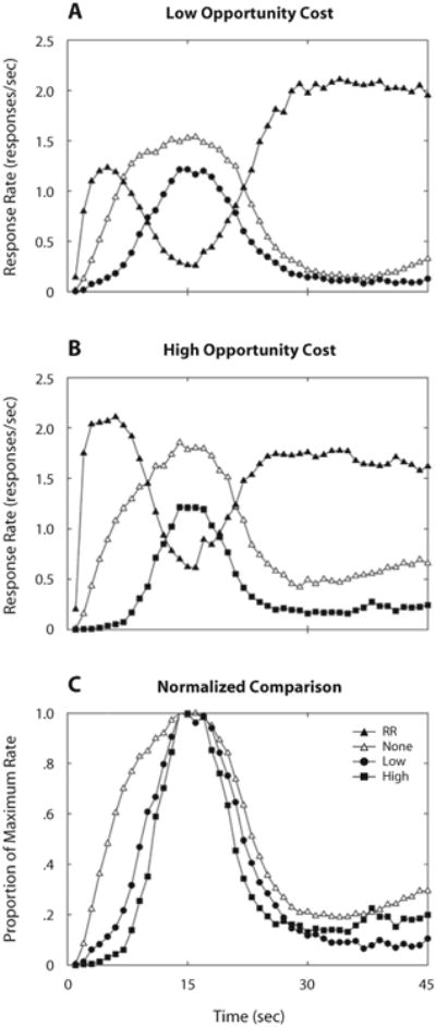
Mean response rates in cost (filled symbols) and no-cost (empty symbols) trials in Experiment 1. Filled triangles represent rates on the RR key; filled circles and squares represent rates on the FI key when opportunity cost was (A) low (r = 1/90) and (B) high (r = 1/30), respectively. (C) Comparison of normalized response rates on the FI key, across opportunity cost conditions. The dispersion of response rates varied inversely with opportunity cost.
Fits of Sanabria and Killeen's (2007) model to no-cost performance did not reveal substantial changes as a function of alternate schedule. Means of the first (∼15-sec) and second (∼60-sec) Gaussians were not substantially different across conditions (p = .92). CVs were not significantly different either (p = .22). Average no-cost CVs were within 9% of Sanabria and Killeen's estimates, which were based on the conventional PI procedure, suggesting that the dispersion of no-cost temporal estimates was typical of PI performance. Although the difference in peak rate of the first Gaussian was not reliable (p > .2), that of the second Gaussian could not be discounted (p = .065). This difference can be observed in the terminal response rate in no-cost trials at the right end of Figures 2A and 2B. Response resurgence was, somewhat surprisingly, slightly greater when opportunity cost was higher. Because the three-state model of PI performance ignores response resurgence, and because we are basing our inferences on estimates of parameters of this model, we will not be concerned with differences in resurgence in this study.
To facilitate visual comparison, normalized response rates were computed as the proportion of keypecks relative to the maximum average response rate. Panel C of Figure 2 compares normalized mean performance on the FI key under different opportunity costs. No-cost performance was averaged. Normalized response rates show an inverse relationship between the dispersion of FI responses and the rate of reinforcement on the alternative schedule. Response rates rose sooner and declined later in no-cost than in cost trials. The effect, however, was not symmetric: Opportunity costs had a stronger effect on the ascending limb of the distribution than on the descending limb.
State Transitions
The temporal locations of low-high and high-low response rate transitions (labeled start time and stop time, respectively) were estimated using a modified version of an analytical procedure employed by Church et al. (1994) and Hanson and Killeen (1981). The response rate at every bin t was modeled as
| (1) |
Equation 1 has five free parameters: s1 and s2 are the estimated start and stop times, and R1, R2, and R3 are the estimated rates in the low, high, and second low states. For every combination of s1 and s2, we set R1, R2, and R3 equal to the mean observed response rate before s1, between s1 and s2, and after s2, respectively. The goodness of fit of each combination was established using the method of least squares. Trials that were best described by a high-low-high pattern (R1 > R2 < R3) were not further analyzed; these trials constituted less than 6% of the total trials for any bird in any condition (M = 3%). Typically, excluded high-low-high trials were better described by a four-state pattern with a terminal high state, which is occasionally observed in the PI procedure (Sanabria & Killeen, 2007).
To validate the three-state model, response rates were averaged across trials after aligning them around transition times, as shown in Figure 3. The assumptions of Equation 1 were supported by the relative flatness of response rates within each state and by the abrupt changes in response rate after each imputed transition time. Between 72% and 78% of the variance in response rates within trials was accounted for by Equation 1 across opportunity cost conditions.
Figure 3.
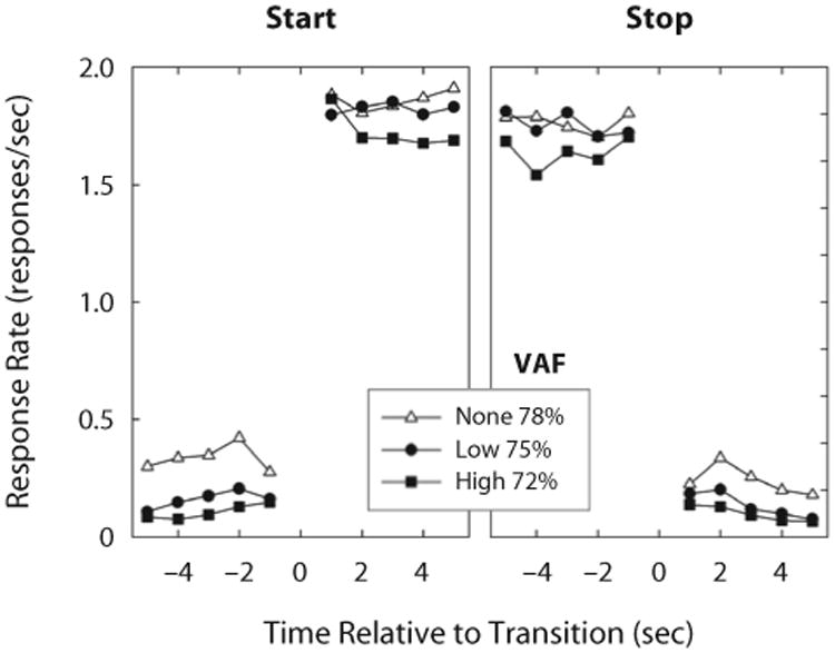
Mean response rates, aligned around start and stop times (left and right panels, respectively), for each opportunity cost condition. Response rates within states shorter than 5 sec were excluded from mean computation. Response rates increased by slightly more than 1.5 responses/sec after start times and decreased by similar magnitudes after stop times; within each state, response rates were relatively constant. Variance accounted for by the three-state model (Equation 1) is reported for each opportunity cost condition.
Figure 4 shows probability distributions of state transitions, averaged across birds. Consistent with results shown in Figure 2, higher opportunity cost yielded distributions that were overall closer to the 15-sec target time (dotted vertical line). Moreover, state transitions were less dispersed—and thus more consistent—with higher opportunity cost.
Figure 4.
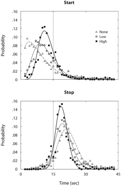
Mean probabilities of starts (top panel) and stops (bottom panel), as a function of time, through a trial in Experiment 1. The symbols designate the opportunity costs for timing. The vertical dotted lines mark the criterial time, 15 sec. Curves are gamma densities fitted to data from each opportunity cost condition. Distributions of these transitions move closer to the target time and become less dispersed as opportunity cost increases.
Sensitivity of transition times to opportunity cost shown in Figure 4 was confirmed by changes in the means and standard deviations of start and stop times, as shown in Table 2. When regressed over r, these statistics showed reliable trends in the directions suggested by Figure 4: a positive slope over opportunity cost for start times, and a negative slope for stop times and for the standard deviations of start and stop times. This means that, as the probability of a reinforced peck in the RR schedule increased across conditions, pecking on the FI key started later (Figure 4, top panel) and stopped earlier (Figure 4, bottom panel), and start and stop times varied less across trials.
Table 2. Transition Times and Derived Measures in Experiment 1.
| Opportunity Cost | |||||||
|---|---|---|---|---|---|---|---|
|
|
|||||||
| None | Low | High | |||||
|
|
|
|
|||||
| Statistic | M | SEM | M | SEM | M | SEM | Slopea |
| Mean | |||||||
| Start time | 9.51 | 1.27 | 11.81 | 0.70 | 12.46 | 0.47 | 80.15** |
| Stop time | 22.22 | 0.94 | 20.40 | 0.48 | 19.07 | 0.57 | − 89.60** |
| Width | 12.72 | 0.66 | 8.60 | 0.82 | 6.61 | 0.81 | − 169.75** |
| Midpoint | 15.87 | 1.06 | 16.11 | 0.44 | 15.77 | 0.32 | −4.73 |
| Standard Deviation | |||||||
| Start time | 6.16 | 0.74 | 5.98 | 0.50 | 4.97 | 0.58 | − 36.99* |
| Stop time | 5.63 | 0.50 | 5.41 | 0.38 | 4.19 | 0.35 | −45.08** |
| Width | 5.85 | 0.66 | 4.91 | 0.34 | 3.46 | 0.39 | −70.71** |
| Midpoint | 5.13 | 0.54 | 5.14 | 0.43 | 4.26 | 0.44 | −28.01* |
| Pearson's r | |||||||
| Start, stop | .51 | 0.04 | .62 | 0.05 | .72 | 0.05 | 6.02** |
| Start, width | − .55 | 0.04 | − .53 | 0.03 | − .53 | 0.07 | 0.46 |
| Log-Odds Ratio of Errorsb | |||||||
| Late starts | − 3.03 | 0.74 | − 1.88 | 0.35 | −2.08 | 0.48 | 23.19 |
| Early stops | −4.48 | 0.82 | − 3.09 | 0.31 | − 3.73 | 0.88 | 15.08 |
Obtained from linear regression of statistic over rate of reinforcement, which ranged from r = 0 to r = 1/30 reinforcers/peck.
Computed as the log2 of the following ratios: f (s1 > 15):f (s1 < 15) for late starts, and f(s2 < 15):f(s2 > 15) for early stops, wheref(g) is the frequency of inequality g.
p < .05.
p < .01.
Table 2 also shows distribution indexes of the widths and midpoints of high-response-rate states. Widths were computed as s2 – s1, and midpoints were computed as (s1 + s2)/2. In accordance with changes in transition times, the high state was narrower with higher opportunity cost, but the midpoint of the high state was not systematically affected; it hovered slightly above the target time of 15 sec in all opportunity cost conditions. As with transition times, widths and midpoints were more consistent with higher opportunity costs.
If start and stop times had been determined by a single underlying Poisson process, as suggested by the good fits of the gamma densities in Figure 4, the standard deviations of start times would be lower than the standard deviations of stop times; more precisely, the differences of their variances would be expected to be equal to the variance of widths (Killeen & Fetterman, 1993). Contrary to these expectations, the mean standard deviation of stop times was lower than the mean standard deviation of start times, regardless of opportunity cost. A single Poisson process also predicts that the correlation between start and stop times would be the square root of the ratio of start-time variance to the sum of start-time and width variance (.72, .77, and .82 for no, low, and high opportunity costs, respectively); no correlation would be expected between start times and widths (Killeen & Fetterman, 1993). Table 2 shows, however, that start–stop correlations were lower than predicted by a Poisson process, and that there was a substantial negative correlation between start times and widths. Start–stop correlations showed a positive trend over opportunity costs, but start–width correlations did not. This indicates that, regardless of opportunity cost, when pigeons started pecking early in the trial, they pecked for a longer time.
Consider, finally, the impact of opportunity cost on FI schedule control. Two types of error were indicative of poor FI schedule control: late starts and early stops. Late starts were defined as trials with start times longer than 15 sec; early stops were defined as trials with stop times shorter than 15 sec. The prevalence of these errors is visible in Figure 4. The probabilities to the right of the dotted line in the top panel represent late starts; those to the left of the dotted line in the bottom panel represent early stops. Log-odds ratios were computed for each type of error as the log base 2 of the number of error trials per normal trial. Normal-start trials were those with start times s1 < 15 sec; normal-stop trials were those with stop times s2 > 15 sec. Thus, a log-odds ratio θ for starts (or stops) indicates that there were 2θ late starts (or early stops) per normal start (or stop). Negative log-odds ratios shown in Table 2 indicate that there were more normal than error trials, consistent with Figure 4: between 4 and 8 normal starts per late start, and between 9 and 22 normal stops per early stop. Late starts were more prevalent than early stops, regardless of opportunity cost. Regressions on r showed no reliable linear trends.
Discussion
Opportunity cost of timing was varied by manipulating the rate of reinforcement programmed in a concurrent schedule. Higher opportunity costs changed start and stop times in directions consistent with reinforcement optimization: With higher opportunity costs, timing responses were closer to target time, and transitions in and out of the FI key were more consistent.
Interestingly, our findings are inconsistent with data on the performance of rats in a preparation similar to ours, as reported by Rider (1981). In that experiment, rats were exposed to concurrent FI variable ratio (VR) schedules of reinforcement. As in our experiment, VR schedules maintained a constant probability of reinforcement in one key; but unlike in our experiment, reinforcement on the VR schedule did not reset the FI: VR and FI schedules were independent. The effect reported by Rider is the opposite of what would be expected from having viewed Figure 2C: A larger proportion of leverpresses happened earlier in FIs 50 and 100 sec, with larger rates of reinforcement on the concurrent VR schedule. Although the use of different species may account for part of these inconsistent results, theoretically more meaningful factors may also play a role. The contrary results obtained by Rider may be due to the difficulty of timing an FI when it is interrupted by reinforcement from the VR, because such reinforcers can be a potent signal to reset the internal clock (Staddon, 1974). Another candidate factor is the longer FI used by Rider. Consequently, in Experiment 2, the enhancement effect of opportunity cost was evaluated over two FI schedules.
A more detailed examination of start and stop times and their derived measures provides some insights into how opportunity costs and other motivational manipulations may be integrated into a model of interval timing. Two standard motivational manipulations, reinforcer size and level of deprivation, have shown inconsistent effects: Larger reinforcers have yielded temporal estimates that are shorter than (Ludvig et al., 2007), longer than (Belke & Christie-Fougere, 2006), or essentially equal to (Kacelnik & Brunner, 2002; Roberts, 1981) those observed with smaller reinforcers. Plowright and colleagues (2000) showed that response rates in pigeons peak earlier when they are hungry; Kacelnik and Brunner (2002) did not replicate this effect with hungry starlings. Motivational manipulations may shift means and variances, but at least the former are quickly recalibrated (Killeen, Hall, & Bizo, 1999; MacEwen & Killeen, 1991; Morgan, Killeen, & Fetterman, 1993). Competing schedules of positive and negative reinforcement have clearer effects on peak timing indexes (K. Cheng, 1992; Matell & Portugal, 2007). Our results replicate the improvement in timing indexes displayed by Matell and Portugal's rats when a concurrent schedule of reinforcement was in place. However, we saw a more reliable effect on stop times than did Matell and Portugal.
Matell and Portugal (2007) interpreted their results as indicating that opportunity cost discourages early impulsive responses in the PI procedure but has no effect on stop times. According to this hypothesis, impulsivity and timing are confounded in start times, thus inducing premature and highly variable start times, but leaving the decision to stop unaffected. Impulsivity would explain the higher variability of start times relative to that of stop times in the PI procedure. Matell and Portugal's account, however, does not explain the changes in the mean and standard deviation of stop times with opportunity cost that they obtained (although not at statistically significant levels), which were again demonstrated more robustly in the present experiment.
A model of PI timing with opportunity cost must thus account for the improvement in timing indexes, regarding not only when time-sensitive pecking starts, but also when it stops. Before we elaborate on such a model, however, we must consider the contingencies of reinforcement that constitute the opportunity cost of timing. In Experiment 1, the opportunity cost of every peck on the FI key was constant, because the probability that a peck on the RR key would be reinforced was constant if the RR schedule was effective. Opportunity cost may be instantiated in many other ways. Indeed, it is unclear how the cost of not engaging in interim activities would be structured over the cycle between reinforcers in no-cost trials; for instance, focal postreinforcer search may be more difficult to disrupt than spontaneous pacing or grooming, and, thus, the opportunity cost of PI timing may decrease as the target time approaches. In Experiment 2, we will consider a scenario where opportunity cost is not constant but, rather, increases with time spent on the FI schedule.
Experiment 2
Peak Timing With a Concurrent Interval Schedule
In Experiment 2, we introduced two variations from Experiment 1. First, we established an opportunity cost with an interval schedule presented concurrently with the FI schedule. In random interval (RI) schedules, reinforcement was set up with constant probability over time, and a response was required in order to collect reinforcers. In contrast to RR schedules, the probability that the next peck in an RI schedule is reinforced is not constant, but increases proportionately with the time since the last peck on the RI schedule. This is analogous to the situation of a forager that has to choose between patches of prey: The density of prey in the patch not chosen may increase with time spent away from it. As instantiated in Experiment 2, the PI procedure with opportunity cost may be described as a choice between a patch that may replenish at any time (RI) and one that fully replenishes after a fixed time (FI).
Method
Subjects and Apparatus
The same 6 pigeons from Experiment 1 were kept under the same housing and feeding conditions. Experiment 2 was conducted after the completion of Experiment 1, using the same apparatus.
Procedure
Experimental sessions were conducted as described for Experiment 1. The cost/no-cost multiple-schedule structure used in Experiment 1 was retained across experimental conditions. In cost trials, the RR schedule was changed to a tandem random-time 5T fixed ratio 5 (TAND [RT 5T, FR 5]), where T could be 15 or 60 sec, depending on the experimental condition (Figure 5).1 During cost trials, every second a probability generator initiated an FR 5 schedule with probability 1/(5T). There was no stimulus change signaling the initiation of the FR 5 schedule, after which the fifth peck on the left-green key was reinforced. The time limit for each TAND trial was set at 6T.
Figure 5.

Diagram of cost and no-cost components in Experiment 2. Rate of reinforcement in TAND and FI keys was a multiple of T, with T = 15 sec, as in Experiment 1, or T = 60 sec. The right response key served as the FI key in both components. Diamonds indicate selection between actions with probabilities p and q = 1 – p. ITI, intertrial interval.
The FI key in cost and no-cost trials functioned similarly to that in Experiment 1, but the criterial time could be T = 15 or 60 sec, depending on the experimental condition. When EXT was operational, a trial finished after 3T of initiation; when FI T was operational, a trial finished after 6T of initiation if there were no effective responses. Cost and no-cost trials that exceeded 2T were deemed “long” for alternation and analysis purposes.
Experimental conditions comprised two variations of the basic procedure: During tandem training, the FI key was dark, and it was not operative in cost trials; in opportunity cost conditions, the FI key was operative concurrently with the TAND key in cost trials, as sketched in Figure 5. The order in which conditions were conducted and the number of sessions in each condition are indicated in Table 3.
Table 3. Order of Presentation and Number of Sessions in Each Condition of Experiment 2.
| (Order) Number of Sessions | ||||||
|---|---|---|---|---|---|---|
|
|
||||||
| Condition | P-105 | P-106 | P-107 | P-110 | P-116 | P-119 |
| Tandem training (T = 15 sec, RT = 75 sec) | (1) 5 | – | – | (1) 5 | (1) 5 | – |
| Tandem training (T = 60 sec, RT = 300 sec) | – | (1) 5 | (1) 5 | – | – | (1) 5 |
| Concurrent tandem schedule* (T = 15 sec, RT = 75 sec) | (2) 30 | (3) 29 | (3) 29 | (2) 30 | (2) 30 | (3) 32 |
| Concurrent tandem schedule* (T = 60 sec, RT = 300 sec) | (3) 29 | (2) 30 | (2) 30 | (3) 32 | (3) 31 | (2) 30 |
Experimental conditions used in data analysis.
Data Analysis
As in Experiment 1, response rates were computed from performance in long trials—those longer than 2T in duration—of the last five sessions of each experimental condition. State transition time estimates were based on the distribution of response rates, as described in Experiment 1. Sensitivity of timing variables to opportunity cost was established using CIs around the difference between variables across opportunity cost conditions. When a CI did not cover zero, the corresponding variable was deemed sensitive to the opportunity cost manipulation. Tests were conducted using 95% and 99% CI (p < .05 and p < .01, respectively).
Results
Response Rates
Figure 6 shows mean response rates as a function of time through trials. Panels A and B show that pigeons pecked mostly on the TAND key at the beginning of cost trials (filled symbols), switched to pecking mostly on the FI key around the target time T, and returned to pecking mostly on the TAND key after the target time elapsed. After T = 60 sec, FI pecking decayed at a substantially slower pace than after T = 15 sec. FI pecks in no-cost trials (empty symbols) followed a similar temporal pattern but were emitted at a higher rate than in cost trials.
Figure 6.
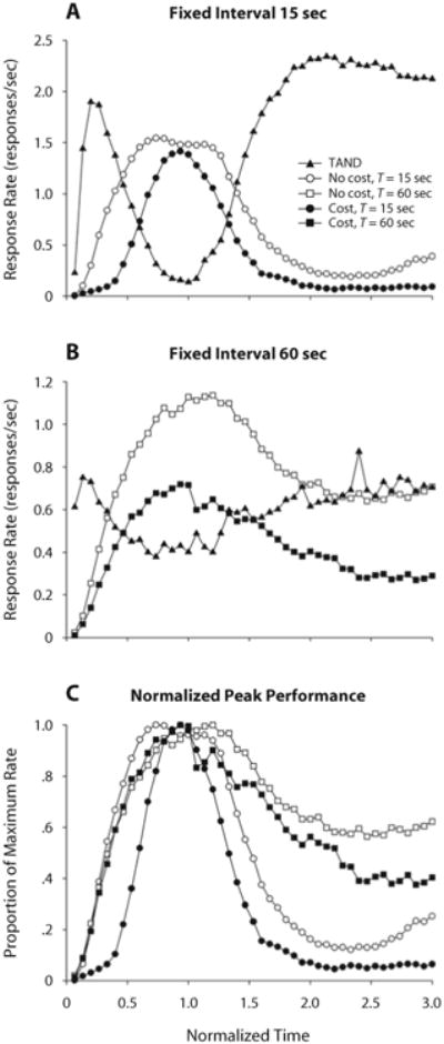
Mean response rates in cost (filled symbols) and no-cost (empty symbols) trials in Experiment 2. The abscissae were normalized by dividing the real time by T. Filled triangles represent rates on the TAND key; filled circles and squares represent rates on the FI key when criterial time T = 15 (panel A) and 60 sec (panel B), respectively. Note the different scales for the ordinates. (C) Comparison of normalized response rates on the FI key, across opportunity costs and criterial times.
Panel C of Figure 6 shows FI response rates as proportions of their maxima. This normalization shows that FI responses were more dispersed when there was no opportunity cost than when there was a cost. In FI 60 sec, dispersion was reduced by opportunity cost only on the right of the normalized distribution; in FI 15 sec, the reduction in dispersion was more symmetrical.
State Transitions
Start and stop times were determined using the procedure described in Experiment 1. Figure 7 shows probability distributions of state transitions for each criterial time T, averaged across birds. When T = 15 sec, opportunity cost induced distributions that were less dispersed and generally closer to T. In contrast, when T = 60 sec, neither starts nor stops showed reduced dispersions with opportunity cost; stops, but not starts, were closer to T.
Figure 7.
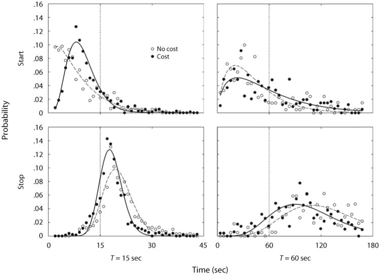
Mean probabilities of starts (top panels) and stops (bottom panels), as a function of time, through a trial in Experiment 2. The vertical dotted lines mark the criterial times: 15 sec (left panels) and 60 sec (right panels). The symbols designate the opportunity costs for timing. The curves are fitted gamma densities.
Table 4 shows that, across T = 15 and T = 60 sec, there were similar changes in transition times and in derived measures over cost and no-cost conditions. When there was an opportunity cost, stop times and widths were reduced, and the correlation between start and stop times increased, regardless of T. Also with opportunity cost, the standard deviation of widths decreased, and the ratio of error to normal trials increased for both criterial times, but statistical significance was reached only by the former effect in T = 15, and only by the latter in T = 60 sec.
Table 4. Transition Times and Derived Measures in Experiment 2.
| T = 15 sec | T = 60 sec | |||||||||
|---|---|---|---|---|---|---|---|---|---|---|
|
|
|
|||||||||
| No Cost | Cost | No Cost | Cost | |||||||
|
|
|
|
|
|||||||
| M | SEM | M | SEM | Difference | M | SEM | M | SEM | Difference | |
| Mean | ||||||||||
| Start time | 9.06 | 2.05 | 10.68 | 1.18 | 1.62 | 49.75 | 9.16 | 56.43 | 6.08 | 6.68 |
| Stop time | 20.69 | 1.26 | 18.34 | 0.59 | −2.35* | 115.76 | 5.57 | 96.37 | 2.61 | − 19.39** |
| Width | 11.63 | 0.97 | 7.66 | 0.76 | − 3.97** | 66.01 | 8.71 | 39.94 | 6.75 | −26.07** |
| Midpoint | 14.88 | 1.63 | 14.51 | 0.85 | −0.37 | 82.75 | 6.20 | 76.40 | 3.24 | − 6.35 |
| Standard Deviation | ||||||||||
| Start time | 4.40 | 0.73 | 4.68 | 0.74 | 0.29 | 32.74 | 6.27 | 38.13 | 1.80 | 5.39 |
| Stop time | 4.61 | 0.59 | 4.29 | 0.41 | −0.32 | 34.80 | 3.90 | 35.20 | 2.31 | 0.40 |
| Width | 4.94 | 0.38 | 3.46 | 0.32 | − 1.48** | 33.98 | 3.80 | 30.94 | 3.25 | − 3.04 |
| Midpoint | 3.78 | 0.62 | 4.15 | 0.56 | 0.37 | 29.55 | 4.43 | 33.19 | 1.66 | 3.64 |
| Pearson's r | ||||||||||
| Start, stop | 0.36 | 0.07 | 0.70 | 0.03 | 0.33** | 0.50 | 0.08 | 0.64 | 0.06 | 0.14* |
| Start, width | −0.51 | 0.08 | −0.45 | 0.06 | 0.06 | −0.41 | 0.11 | −0.50 | 0.05 | −0.09 |
| Log-Odds Ratio of Errorsa | ||||||||||
| Late starts | − 3.59 | 1.17 | − 3.32 | 0.92 | 0.27 | − 1.81 | 0.84 | −0.67 | 0.41 | 1.14* |
| Early stops | − 3.88 | 0.75 | −2.73 | 0.59 | 1.15 | −4.34 | 0.41 | −2.62 | 0.28 | 1.73** |
Discussion
In Experiment 1, where opportunity cost was effected by an RR schedule, increasing cost enhanced a broad range of timing indexes; timing responses clustered more tightly around the target time, and transitions into and out of the timed response were crisper. In Experiment 2, opportunity cost was effected by an RI schedule. In such schedules, cost increases as pigeons allocate more pecking on the timing task. Most of the effects detected in Experiment 1 were replicated in Experiment 2, although some replications did not achieve statistical significance. Regardless of whether opportunity costs were arranged as ratio or interval schedules, and across two criterial times, opportunity cost had similar effects: Transitions in and out of high response rate states occurred closer to the target time, thus narrowing the width of the state of high responding; the midpoint of the high state remained relatively unchanged. Contrary to expectations from the impulsivity hypothesis advanced by Matell and Portugal (2007), opportunity cost did not always result in more precise start times (Table 4); it primarily contributed to more precise widths. Pigeons were not necessarily more consistent in when they started pecking, but were so in how long they continued pecking.
The primacy of the how long over the when effect, seen in the decrease of the standard deviation of high-state widths in all conditions, is consistent with the enhanced correlation between starts and stops with opportunity cost: If opportunity cost reduced start variability (but not width variability), the correlation between starts and stops would decrease; but, in fact, it systematically increased. It is also important to note that, whereas in Experiment 1 the standard deviations of starts and widths were reduced with opportunity cost, in Experiment 2 no reduction was observed for starts—only for widths. This difference may be related to the increased probability of reinforcement on the TAND key, after leaving the FI key. When the ratio schedule of Experiment 1 was effective, a keypeck on the RR key was just as likely or unlikely to be reinforced after subjects had spent a substantial amount of time on the FI key as at any other time; in contrast, when the interval schedule of Experiment 2 was effective, a keypeck on the TAND key was more likely to be reinforced after spending a substantial time on the FI key than when the TAND key was recently pecked. More reliable reinforcement after leaving the FI key may have induced the shorter and more consistent stop times in Experiment 2 (T = 15 sec) as compared with those in Experiment 1.
Consistent with data from Experiment 1, the improvement in timing indexes driven by opportunity cost in Experiment 2 also resulted in less efficient collection of FI reinforcers. The bottom rows of Table 4 show that when transition times were closer to the target time, this shift was not compensated by a sufficient reduction in dispersion of transition times, so more of the tail of the distributions fell on the error sides of the target time; there were proportionately more late starts and early stops. The cost-driven reduction in FI efficiency, however, may have facilitated the efficient collection of reinforcers in the alternate schedule, which may have yielded an overall optimal rate of reinforcement under constraints imposed by the timing and motor capacities of the pigeons.
As also demonstrated in Experiment 1, a single Poisson process cannot account for the standard deviations and correlations of start and stop times in Experiment 2. The difference in the standard deviations of starts and stops was substantially smaller than the variance of widths. Based on start-time and width variances, a single Poisson process predicts start-stop correlations under T = 15 sec of .66 and .80, for the no-cost and cost conditions, respectively, and of .69 and .78 under T = 60 sec; obtained correlations were between .08 and .30 below predictions. A single Poisson process predicts no correlation between start times and width; as in Experiment 1, we observed a substantial negative correlation between when pigeons started pecking and how long they continued pecking. The transition analysis by Killeen and Fetterman (1993) improves the predictions, but not enough to justify the extra parameter it entails.
General Discussion
In summary, more precise and more accurate start and stop times in the PI procedure may be motivated by opportunity costs. This suggests that conventional PI data must be interpreted with caution, because timing indexes derived from PI performance are likely to confound timing and motivational variables. Time-production processes may be better studied using reinforcement that punishes poor performance. Prior research indicates, however, that alternate reinforcement, interspersed within the timing interval, may actually impair rather than enhance timing (Nevin, 1971; Rider, 1981; Staddon, 1974). We expect that clearly discriminable alternate reinforcement that does not occur within the timed interval—that restarts the interval to be timed, rather than merely interrupting it—will enhance the timing of that interval, as demonstrated here.
Single-trial analyses of PI performance have reliably shown that starts are negatively correlated with widths and positively correlated with stops (Church, Meck, & Gibbon, 1994; Gibbon & Church, 1992). The start–width correlation was shown here to be immune to opportunity cost, but the start–stop correlation increased with higher opportunity cost. This increase suggests that opportunity cost primarily reduced the variability of how long the FI key was engaged; it only secondarily affected the variability of when FI responding started. The distinction between processes that affect starts, widths, and stops may have important consequences for neurobiological accounts of timing (Ludvig et al., 2007; K. M. Taylor et al., 2007).
The mechanisms underlying cost-driven improvement in timing are still obscure. One possibility is that differences in overall rate of reinforcement—which increased with opportunity cost—are responsible for the effects reported here. The behavioral theory of timing predicts that pulses, whose accumulation serves as an index of time, are emitted at a higher rate when reinforcement increases (Bizo & White, 1995; Killeen & Fetterman, 1988; MacEwen & Killeen, 1991; Morgan, Killeen, & Fetterman, 1993). To maintain accuracy, more pulses are accumulated, which results in a slimmer (Erlang) distribution of temporal estimates. This change in distribution may be comparable to those shown in panel C of Figures 2 and 6. Nonetheless, the observed sensitivity of start and stop times to rate of reinforcement has not been specified in this theory of timing. There is no obvious map relating changes in overall reinforcement with the observed changes in start and stop times. A simpler model may assume that start and stop decisions are linked to sources of reinforcement: If the probability of reinforcement becomes higher in source A than in source B, then source A starts being exploited and source B stops being exploited. We built a timing model that incorporates opportunity cost by formalizing this parsimonious rule.
A Model of Opportunity Cost of Timing
An optimal forager in the paradigms used in our experiments should respond on the alternate key (RR in Experiment 1, TAND in Experiment 2), as long as the probability of reinforcement there exceeds that on the FI key. This entails continual responding on the alternate key until criterial time T, emitting one response on the FI key, and then returning to the alternate key. But no organism can time an interval so precisely. We may adopt one of the standard timing models, involving a cumulative gamma or normal distribution, to trace the subjective probability that 15 sec have elapsed against real time. If the FI and alternate schedules were concurrently available, the animal should switch when the probability that T has elapsed just exceeds the probability of reinforcement for a response on the alternate schedule—1/30 or 1/90, in Experiment 1. With each unreinforced response on the RR key, and with each second spent pecking on the TAND key, it becomes more likely that the FI key will be effective in that trial. This gives an additional incentive to switch out of the alternate key to the FI, if the animals are sensitive to this information. The same consideration is, to a lesser extent, true for the FI key. Killeen, Palombo, Gottlob, and Beam (1996) developed a Bayesian model of patch choice along such lines. Here, the data do not discriminate between that model and the following, much simpler one, analogous to a model suggested by Staddon (1977): Switch to the FI when the probability that the next peck will be reinforced just exceeds the probability that it will be reinforced on the alternate schedule. That is, switch in when
| (2) |
The function on the left of Equation 2 is the cumulative normal distribution, giving the cumulative probability that the interval has elapsed at any time t according to the animal's sense of time; the imprecision of such sense of time is proportional to the interval timed, following Weber's law. Following the behavioral theory of timing (Killeen & Fetterman, 1988), tighter distributions (i.e., lower c values) may be expected with higher rates of reinforcement. The probability distribution is weighted by pFI, the probability that FI reinforcement will be scheduled: In our experiments, pFI = 1/2 on cost trials and 2/3 on no-cost trials. The variable on the right of Equation 2 is the probability of reinforcement under the competing schedule.
Just as animals should switch in to the FI when their estimate of the probability that t ≥ T exceeds r, they should switch out of the FI schedule when the probability that it is in force decreases below r. As time elapses with responding on the FI key, it becomes increasingly unlikely that the FI is primed on that trial. It is reasonable to make this inference as a function of the complement of the normal timing distribution: If you are, say, 90% certain that food would have come by now if it had been primed, then—taking base rates into account—you should switch out of FI when
| (3) |
The model is sketched in Figure 8. To evaluate it, we formulated predictions and contrasted them with the data from Experiments 1 and 2, as well as from Matell and Portugal's (2007) study. For Experiment 1, we set ri to the probability of reinforcement on the RR key when it was effective—1/30 and 1/90. For Experiment 2, we derived the probability of reinforcement, ri, from the assumption that it was approximately equal to the rates of reinforcement—1/75 and 1/300 sec−1—divided by the asymptotic TAND response rates—2.5 and 0.7 responses/sec, respectively—for T = 15 sec and T = 60 sec. We used a similar procedure to estimate ri in Matell and Portugal's study, extracting an asymptotic response rate equal to 0.5 responses/sec from their Figure 3A. There were no experimenter-arranged competing reinforcers in the no-cost conditions, so a naive prediction is that the animals should respond continually on the FI schedule. That they do not suggests that there were at least some minimally competitive activities in the environment that were more reinforcing, and thus competed effectively with FI responding both early and late in the interval. We imputed such reinforcers as being delivered with a probability r0. Figure 9 shows model predictions from fitting to data a separate μ for each T condition, a single coefficient of variation c, and a single value of r0. Predictions followed relatively closely to the data, and no systematic deviations were evident.
Figure 8.
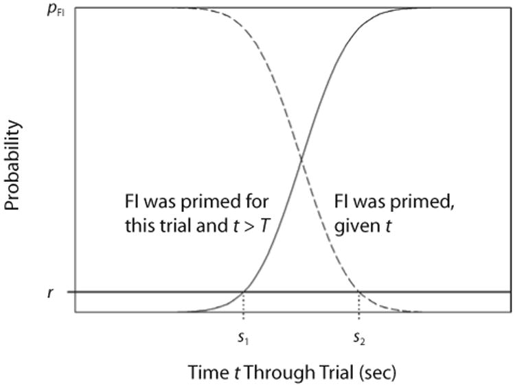
Opportunity cost model. Starts (s1) occur when the subjective probability of fixed-interval (FI) reinforcement exceeds the probability of reinforcement in the alternate schedule (r). Stops (s2) occur when the probability that FI was primed falls below r.
Figure 9.
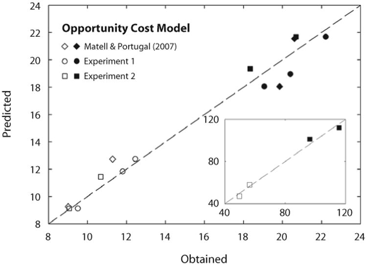
Obtained starts (empty symbols) and stops (filled symbols) in three experiments, plotted against predictions from the opportunity cost model (Equations 2 and 3 in the text). The plot for T = 60 sec in the present Experiment 2 is shown in the inset. Parameters of the model were μ15 = 15.4 sec, μ60 = 79.5 sec, r0 = 1.3 × 10⁻⁴; for all data, c = 0.12.
The account we propose here is necessarily incomplete; for instance, the decision to start timing must be a convolution of where the animal estimates it is in time at any t and its estimation of what the target time is. Equations 2 and 3 do not address the observed changes in variance and covariance that were driven by opportunity cost. Nonetheless, the simplicity of that analysis makes it a decent starting point for more sophisticated timing models. In particular, note that the CV of temporal estimates, c, is constant over T and over the nature of the competing reinforcement schedule. It is less than half the magnitude of the CV of midpoints, and it compares favorably to that of humans in temporal discrimination tasks (Fetterman & Killeen, 1992; Grondin, 2001). The model does not require that the distribution of response rates be bell shaped, and often they are not. It does not base inferences on the response rates within high states, because those are often contingent upon the time at which the animal starts responding (Hanson & Killeen, 1981). Finally, it may be applied to other constellations of arrangements, such as traditional FI schedules, and to mixed FI schedules, such as those studied by Catania and Reynolds (1968).
Herrnstein's (1961, 1970) seminal research on concurrent variable-interval schedules broadened our understanding of how reinforcers operate on behavior by manipulating contextual reinforcement. A similar manipulation appears to be critical to the advancement of our knowledge of the processes involved in temporal production. We have demonstrated that peak performance on a single operandum is intrinsically limited in discriminating timing from motivational processes. The experimental control of contextual reinforcement using multiple operanda overcomes these limitations. The opportunity cost model provides a first-order approximation of the role of contextual reinforcement on timing.
Acknowledgments
E.A.T. is currently at Utah State University, Logan, UT. This research was supported by NSF Grant IBN 023682 and NIMH Grant 1R01MH0 66860 to P.R.K. We thank Matthew T. Sitomer and Lewis A. Bizo for their invaluable advice at early stages of this project, and Weihua Chen for analyzing the preliminary data. Randolph C. Grace and two anonymous reviewers provided helpful comments on an early draft of this article. Portions of this research were presented at the 2005 meeting of the Society for Quantitative Analysis of Behavior and at the 2007 meeting of the Psychonomic Society.
Footnotes
Note: A TAND [RT x, FR 1] schedule is equivalent to an RI x schedule. The TAND schedule used in Experiment 2 is equivalent to an RI 5T schedule, where reinforcement had to be collected with five keypecks, not just one. This manipulation typically enhances and regularizes response rates.
References
- Asgari K, Body S, Zhang Z, Fone KCF, Bradshaw CM, Szabadi E. Effects of 5-HT1A and 5-HT2A receptor stimulation on temporal differentiation performance in the fixed-interval peak procedure. Behavioural Processes. 2006;71:250–257. doi: 10.1016/j.beproc.2005.06.007. [DOI] [PubMed] [Google Scholar]
- Belke TW, Christie-Fougere MM. Investigations of timing during the schedule and reinforcement intervals with wheel-running reinforcement. Behavioural Processes. 2006;73:240–247. doi: 10.1016/j.beproc.2006.06.004. [DOI] [PubMed] [Google Scholar]
- Bizo LA, White KG. Biasing the pacemaker in the behavioral theory of timing. Journal of the Experimental Analysis of Behavior. 1995;64:225–235. doi: 10.1901/jeab.1995.64-225. [DOI] [PMC free article] [PubMed] [Google Scholar]
- Brodbeck DR, Hampton RR, Cheng K. Timing behaviour of black-capped chickadees (Parus atricapillus) Behavioural Processes. 1998;44:183–195. doi: 10.1016/S0376-6357(98)00048-5. [DOI] [PubMed] [Google Scholar]
- Catania AC. Reinforcement schedules and psychophysical judgments: A study of some temporal properties of behavior. In: Schoenfeld WN, editor. The theory of reinforcement schedules. New York: Appleton-Century-Crofts; 1970. pp. 1–42. [Google Scholar]
- Catania AC, Reynolds GS. A quantitative analysis of the responding maintained by interval schedules of reinforcement. Journal of the Experimental Analysis of Behavior. 1968;11:327–383. doi: 10.1901/jeab.1968.11-s327. [DOI] [PMC free article] [PubMed] [Google Scholar]
- Cheng K. The form of timing distributions in pigeons under penalties for responding early. Animal Learning & Behavior. 1992;20:112–120. [Google Scholar]
- Cheng K, Westwood R. Analysis of single trials in pigeons' timing performance. Journal of Experimental Psychology: Animal Behavior Processes. 1993;19:56–67. doi: 10.1037/0097-7403.19.1.56. [DOI] [Google Scholar]
- Cheng RK, Ali YM, Meck WH. Ketamine “unlocks” the reduced clock-speed effects of cocaine following extended training: Evidence for dopamine–glutamate interactions in timing and time perception. Neurobiology of Learning & Memory. 2007;88:149–159. doi: 10.1016/j.nlm.2007.04.005. [DOI] [PubMed] [Google Scholar]
- Church RM, Meck WH, Gibbon J. Application of scalar timing theory to individual trials. Journal of Experimental Psychology: Animal Behavior Processes. 1994;20:135–155. doi: 10.1037/0097-7403.20.2.135. [DOI] [PubMed] [Google Scholar]
- Davison M, McCarthy D. The matching law: A research review. Hillsdale, NJ: Erlbaum; 1988. [Google Scholar]
- Drew MR, Zupan B, Cooke A, Couvillon PA, Balsam PD. Temporal control of conditioned responding in goldfish. Journal of Experimental Psychology: Animal Behavior Processes. 2005;31:31–39. doi: 10.1037/0097-7403.31.1.31. [DOI] [PubMed] [Google Scholar]
- Ferster CB, Skinner BF. Schedules of reinforcement. New York: Appleton-Century-Crofts; 1957. [Google Scholar]
- Fetterman JG, Killeen PR. Time discrimination in Columba livia and Homo sapiens. Journal of Experimental Psychology: Animal Behavior Processes. 1992;18:80–94. doi: 10.1037/0097-7403.18.1.80. [DOI] [PubMed] [Google Scholar]
- Gallistel CR, Gibbon J. Time, rate, and conditioning. Psychological Review. 2000;107:289–344. doi: 10.1037/0033-295X.107.2.289. [DOI] [PubMed] [Google Scholar]
- Gibbon J, Church RM. Representation of time. Cognition. 1990;37:23–54. doi: 10.1016/0010-0277(90)90017-E. [DOI] [PubMed] [Google Scholar]
- Gibbon J, Church RM. Comparison of variance and covariance patterns in parallel and serial theories of timing. Journal of the Experimental Analysis of Behavior. 1992;57:393–406. doi: 10.1901/jeab.1992.57-393. [DOI] [PMC free article] [PubMed] [Google Scholar]
- Gooch CM, Wiener M, Portugal GS, Matell MS. Evidence for separate neural mechanisms for the timing of discrete and sustained responses. Brain Research. 2007;1156:139–151. doi: 10.1016/j.brainres.2007.04.035. [DOI] [PubMed] [Google Scholar]
- Grondin S. From physical time to the first and second moments of psychological time. Psychological Bulletin. 2001;127:22–44. doi: 10.1037/0033-2909.127.1.22. [DOI] [PubMed] [Google Scholar]
- Hanson SJ, Killeen PR. Measurement and modeling of behavior under fixed-interval schedules of reinforcement. Journal of Experimental Psychology: Animal Behavior Processes. 1981;7:129–139. doi: 10.1037/0097-7403.7.2.129. [DOI] [Google Scholar]
- Herrnstein RJ. Relative and absolute strength of response as a function of frequency of reinforcement. Journal of the Experimental Analysis of Behavior. 1961;4:267–272. doi: 10.1901/jeab.1961.4-267. [DOI] [PMC free article] [PubMed] [Google Scholar]
- Herrnstein RJ. On the law of effect. Journal of the Experimental Analysis of Behavior. 1970;13:243–266. doi: 10.1901/jeab.1970.13-243. [DOI] [PMC free article] [PubMed] [Google Scholar]
- Kacelnik A, Brunner D. Timing and foraging: Gibbon's scalar expectancy theory and optimal patch exploitation. Learning & Motivation. 2002;33:177–195. doi: 10.1006/lmot.2001.1110. [DOI] [Google Scholar]
- Killeen PR, Fetterman JG. A behavioral theory of timing. Psychological Review. 1988;95:274–295. doi: 10.1037/0033-295X.95.2.274. [DOI] [PubMed] [Google Scholar]
- Killeen PR, Fetterman JG. The behavioral theory of timing: Transition analyses. Journal of the Experimental Analysis of Behavior. 1993;59:411–422. doi: 10.1901/jeab.1993.59-411. [DOI] [PMC free article] [PubMed] [Google Scholar]
- Killeen PR, Hall S, Bizo LA. A clock not wound runs down. Behavioural Processes. 1999;45:129–139. doi: 10.1016/S0376-6357(99)00014-5. [DOI] [PubMed] [Google Scholar]
- Killeen PR, Palombo GM, Gottlob LR, Beam J. Bayesian analysis of foraging by pigeons (Columba livia) Journal of Experimental Psychology: Animal Behavior Processes. 1996;22:480–496. doi: 10.1037/0097-7403.22.4.480. [DOI] [PMC free article] [PubMed] [Google Scholar]
- Killeen PR, Taylor TJ. How the propagation of error through stochastic counters affects time discrimination and other psychophysical judgments. Psychological Review. 2000;107:430–459. doi: 10.1037/0033-295X.107.3.430. [DOI] [PubMed] [Google Scholar]
- Kirkpatrick K. Packet theory of conditioning and timing. Behavioural Processes. 2002;57:89–106. doi: 10.1016/S0376-6357(02)00007-4. [DOI] [PubMed] [Google Scholar]
- Ludvig EA, Conover K, Shizgal P. The effects of reinforcer magnitude on timing in rats. Journal of the Experimental Analysis of Behavior. 2007;87:201–218. doi: 10.1901/jeab.2007.38-06. [DOI] [PMC free article] [PubMed] [Google Scholar]
- MacEwen D, Killeen PR. The effects of rate and amount of reinforcement on the speed of the pacemaker in pigeons' timing behavior. Animal Learning & Behavior. 1991;19:164–170. [Google Scholar]
- Machado A. Learning the temporal dynamics of behavior. Psychological Review. 1997;104:241–265. doi: 10.1037/0033-295X.104.2.241. [DOI] [PubMed] [Google Scholar]
- Matell MS, Portugal GS. Impulsive responding on the peak-interval procedure. Behavioural Processes. 2007;74:198–208. doi: 10.1016/j.beproc.2006.08.009. [DOI] [PMC free article] [PubMed] [Google Scholar]
- Meck WH. Frontal cortex lesions eliminate the clock speed effect of dopaminergic drugs on interval timing. Brain Research. 2006;1108:157–167. doi: 10.1016/j.brainres.2006.06.046. [DOI] [PubMed] [Google Scholar]
- Morgan L, Killeen PR, Fetterman JG. Changing rates of reinforcement perturbs the flow of time. Behavioural Processes. 1993;30:259–271. doi: 10.1016/0376-6357(93)90138-H. [DOI] [PubMed] [Google Scholar]
- Nevin JA. Rates and patterns of responding with concurrent fixed-interval and variable-interval reinforcement. Journal of the Experimental Analysis of Behavior. 1971;16:241–247. doi: 10.1901/jeab.1971.16-241. [DOI] [PMC free article] [PubMed] [Google Scholar]
- Plowright CMS, Church D, Behnke P, Silverman A. Time estimation by pigeons on a fixed interval: The effect of pre-feeding. Behavioural Processes. 2000;52:43–48. doi: 10.1016/S0376-6357(00)00110-8. [DOI] [PubMed] [Google Scholar]
- Rakitin BC, Gibbon J, Penney TB, Malapani C, Hinton SC, Meck WH. Scalar expectancy theory and peak-interval timing in humans. Journal of Experimental Psychology: Animal Behavior Processes. 1998;24:15–33. doi: 10.1037/0097-7403.24.1.15. [DOI] [PubMed] [Google Scholar]
- Rider DP. Concurrent fixed-interval variable-ratio schedules and the matching relation. Journal of the Experimental Analysis of Behavior. 1981;36:317–328. doi: 10.1901/jeab.1981.36-317. [DOI] [PMC free article] [PubMed] [Google Scholar]
- Roberts S. Isolation of an internal clock. Journal of Experimental Psychology: Animal Behavior Processes. 1981;7:242–268. doi: 10.1037/0097-7403.7.3.242. [DOI] [PubMed] [Google Scholar]
- Sanabria F, Killeen PR. Temporal generalization accounts for response resurgence in the peak procedure. Behavioural Processes. 2007;74:126–141. doi: 10.1016/j.beproc.2006.10.012. [DOI] [PubMed] [Google Scholar]
- Sandstrom NJ. Estradiol modulation of the speed of an internal clock. Behavioral Neuroscience. 2007;121:422–432. doi: 10.1037/0735-7044.121.2.422. [DOI] [PubMed] [Google Scholar]
- Staddon JER. Temporal control, attention, and memory. Psychological Review. 1974;81:375–391. doi: 10.1037/h0036998. [DOI] [Google Scholar]
- Staddon JER. On Herrnstein's equation and related forms. Journal of the Experimental Analysis of Behavior. 1977;28:163–170. doi: 10.1901/jeab.1977.28-163. [DOI] [PMC free article] [PubMed] [Google Scholar]
- Taylor KM, Horvitz JC, Balsam PD. Amphetamine affects the start of responding in the peak interval timing task. Behavioural Processes. 2007;74:168–175. doi: 10.1016/j.beproc.2006.11.005. [DOI] [PubMed] [Google Scholar]
- Taylor PE, Haskell M, Appleby MC, Waran NK. Perception of time duration by domestic hens. Applied Animal Behaviour Science. 2002;76:41–51. doi: 10.1016/S0168-1591(01)00210-6. [DOI] [Google Scholar]
- Yi L. Applications of timing theories to a peak procedure. Behavioural Processes. 2007;75:188–198. doi: 10.1016/j.beproc.2007.01.010. [DOI] [PubMed] [Google Scholar]