

Abstract
In this paper, we describe a model for maximum likelihood estimation (MLE) of the relative abundances of different conformations of a protein in a heterogeneous mixture from small angle X-ray scattering (SAXS) intensities. To consider cases where the solution includes intermediate or unknown conformations, we develop a subset selection method based on k-means clustering and the Cramér-Rao bound on the mixture coefficient estimation error to find a sparse basis set that represents the space spanned by the measured SAXS intensities of the known conformations of a protein. Then, using the selected basis set and the assumptions on the model for the intensity measurements, we show that the MLE model can be expressed as a constrained convex optimization problem. Employing the adenylate kinase (ADK) protein and its known conformations as an example, and using Monte Carlo simulations, we demonstrate the performance of the proposed estimation scheme. Here, although we use 45 crystallographically determined experimental structures and we could generate many more using, for instance, molecular dynamics calculations, the clustering technique indicates that the data cannot support the determination of relative abundances for more than 5 conformations. The estimation of this maximum number of conformations is intrinsic to the methodology we have used here.
I. Introduction
The utility of small angle X-ray scattering (SAXS) to provide structural information was first demonstrated by Guinier's studies of metallic alloys in the late 1930s [1]. SAXS measurements were initially employed to characterize the sizes and shapes of biological macromolecules by Guinier and Fournet in 1955 [2]. Throughout the 60s and 70s, SAXS was widely utilized to study the structures of proteins in solution. However, its popularity decreased due to the inability to extract three-dimensional information from the patterns. Demonstration that SAXS data can be used to establish the low-resolution shape of macromolecules in solution [3] coupled with availability of appropriate synchroton source beam lines has triggered rapid growth of the approach [4]. These methods work for scattering of solutions from proteins (or other macromolecules) that adopt a single conformation in solution. However, in many cases, very interesting biochemical questions arise about the ensemble behavior of proteins in solution under conditions wherein they adopt multiple conformations. In particular, ensembles or mixtures of distinct conformations represent important applications of SAXS [5], [6], [7], and [8]. The goal of these studies may be to determine the relative concentrations and/or the structures of each of the most highly abundant species. To what extent can a single scattering pattern be used to estimate the relative abundances of different conformations in a solution? Here we approach that question using a novel maximum likelihood estimation (MLE) approach and compare the estimates made to those produced by a commonly used existing method.
Proteins are complex molecular machines whose functions often depend on conformational changes, i.e. a “lid” closes to trap a substrate in an enzyme's active site [9]. X-ray crystallography experiments provide atomically detailed “snapshots” of protein structures, enabling many insights into understanding protein structure-function relationships [10]. However, crystal structures offer information on a single protein conformation, a single snapshot selected from the conformational ensembles of structures the protein must adopt during its function [11]. Consequently, conformational states that are biologically important, such as long-lived intermediates along a conformational transition pathway, are difficult to identify by crystallography.
In contrast, small-angle X-ray scattering (SAXS) of protein solutions, and its wide-angle counterpart (WAXS), provide information about protein structure averaged over the ensemble of available structures under any given solution condition, allowing in principle the identification of changes in conformation due to ligand binding [12] or a change in redox state [13]. In particular, if a protein exists in distinct conformational states, then SAXS data will represent, to first order, the weighted combination of the intensity of scattering from each individual state, where the weights are determined by the fraction of the population present in each state. Consequently, SAXS/WAXS experiments that “sweep” a parameter such as temperature [14] or protein concentration [15], to vary the relative abundances of these conformations, offer the possibility of obtaining new insights into protein function.
Directly determining the number of conformations present in a mixture requires a knowledge of the complete state of the protein system, such as energy and temperature. In particular, to calculate the number of conformations, one must be able to partition the energy of an ensemble. However, this is not yet a well-defined problem for a heterogeneous mixture of proteins. If we simplify the problem and only attempt to estimate the relative population of states, then it is well-known in basic thermodynamic principles that they are equal to the ratio of exponentials of the energies of the states to the total energy of the ensemble. However even in this setting, to calculate the relative abundances, it is necessary to know the ratio of the energies among different states in the same environment. However, in practice this prior information about the system isn't known, in which case the best unbiased estimate is to assume that all states are equally likely. In the rest of this manuscript, we follow this assumption.
There are three primary challenges to estimating unknown relative abundances of protein conformations in a mixture solution that must be addressed. First, resolving the identifiability issue in the estimation problem that employs measured data that are numerically badly scaled (i.e. nearly linearly dependent, from a naive analysis) and that include significant noise. Second, obtaining estimation solutions for the conformations that are biophysically interpretable. Third, determining novel, as-yet-unidentified conformational states in addition to the ones that are presently known. There are three main methods commonly used for the estimation of the relative abundances of scattering profiles: (1) the singular-value decomposition (SVD) [11]; (2) MIXTURE [5]; (3) OLIGOMER [5]. While the SVD and MIXTURE methods do not address any of the challenges laid out above, OLIGOMER addresses the second challenge.
Specifically, the SVD determines, in a least squares sense, the minimum number of patterns required to describe an experimental scattering profile by representing the scattering intensity data set matrix as a multiplication of basis vectors weighted by their contributions [11]. It is, of course, a very powerful technique. However it is not robust to noise in the measurements and it results in a basis set in which no member of the set necessarily corresponds to the intensity distribution of an actual structure. Therefore, the SVD method can address none of the challenges mentioned above.
Two publicly available software packages which implement more sophisticated methods to estimate abundances of more physically meaningful structures from SAXS data are MIXTURE and OLIGOMER [5]. The MIXTURE method defines a basis set consisting of droplet or cylindrical functions, or other primitives, to represent the measured SAXS intensities. It finds the relative abundances of members of that basis set for multiple conformational states of a protein through nonlinear curve fitting. Unlike the SVD, with MIXTURE one can resolve a measured intensity from a mixture of particles with simple geometrical shapes containing up to ten different components. In other words, the basis vectors have a geometrical meaning. However, even though interpreting a mixture in terms of a weighted average of given geometrical structures may be valuable in determining rough shapes, this method does not provide a direct explanation of the relative distribution of actual conformations of a protein. Moreover, the non-linear curve fitting approach utilized by MIXTURE does not use information about the measurement noise; therefore it may be susceptible to changes in the noise characteristics. Thus, MIXTURE can not address any of the challenges listed above. On the other hand, the OLIGOMER software can identify different protein conformations utilizing known measured intensities as the basis functions through a non-negative linear least-squares algorithm (NNLSE) for realtive abundance estimation [5], [16]. Even though OLIGOMER addresses the second challenge, by itself NNLSE does not consider the statistical characteristics of the measurement noise and does not attempt to address the identifiability issue in the estimation problem. Therefore, OLIGOMER can not address the first challenge. Moreover, since OLIGOMER uses the intensities of known conformations as the basis vectors, it cannot address the third challenge either.
Here, we propose an approach to the first two challenges only. Specifically, employing SAXS intensity vectors corresponding known conformations of a protein as the basis set and proposing a specific noise model based on both theory and experimental observations, we develop a constrained MLE approach to estimate the relative abundances of multiple conformational states in a protein solution. This approach provides a biophysically interpretable estimation approach that is robust to measurement noise. Moreover, to overcome the identifiability issues in the estimation problem, we develop a basis subset selection method based on the Cramér-Rao bound on the error of estimating relative abundances. The proposed subset selection method finds the subset of intensities for which the total estimation error is minimized. We also show that this subset selection method enables us to choose intensities corresponding to identifiable conformations.
The structure of the rest of this paper is as follows: First, in Section II, we provide background information on SAXS. Then, in Section III, we explain our assumptions on the measured SAXS intensities and accordingly demonstrate the proposed measurement model which incorporates measurement noise and measurement intensities. In Section IV we develop a maximum likelihood based method for estimation of mixture coefficients in the heterogeneous mixture. Then in Section IV-A we describe a subset selection method which uses k-means clustering of SAXS intensities of conformations identified through X-ray crystallography and the Cramér-Rao bound on mixture coefficient estimation error to choose a sparse set of intensities that are sufficient to represent a subset of intensities which correspond to conformations that are identifiable from the data. Finally, in Section V, we use the 45 known conformations of adenylate kinase (ADK) to provide a computational example to demonstrate the estimation performance of the proposed method and compare it to that of OLIGOMER on the same data.
II. Small Angle X-Ray Scattering
A typical SAXS experiment is illustrated in Figure 1. In SAXS experiments, a circular average of X-ray intensities from a solution is measured, which we can represent as follows:
Fig. 1.
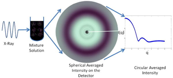
SAXS experiments are, in principle, very simple: A monochromatic x-ray beam is incident on a solution containing proteins that may take on multiple conformations. X-ray scattering is collected on a two-dimensional detector and those intensities are circularly averaged and scaled taking into account the geometry of the experiment, in particular, the sample to detector distance and wavelength of the incident x-rays.
| (1) |
where A(q) is the 3D Fourier transform of the excess electron density Δρ(r) with r = [x, y, z] as the Cartesian coordinates in laboratory frame, and q = (q,Ω) is the scattering vector in terms of scattering coordinates in reciprocal space with q ∈ [qmin, qmax]. qmin and qmax depend on the experimental conditions and the dimensions of the detector array, Ω is the solid angle in reciprocal space, and A(q) can be computed using
| (2) |
where Vr is the total volume of molecule and a thin hydration layer [18]. Circularly averaged SAXS intensity is then calculated using
| (3) |
where,
| (4) |
dmax is the diameter of the smallest sphere that would contain the molecule hydrational layer and γ(r) is the spherically averaged autocorrelation function of the excess electron density [3]. In this paper, we use the software package CRYSOL [19] to calculate SAXS intensities of known conformations of a protein [3]. CRYSOL starts from atomic coordinates in a protein data base (PDB) file and calculates the SAXS intensities taking into account the hydration layer. Specifically, it calculates the Fourier transform of the excess electron densities employing spherical Bessel functions and spherical harmonics in the range of scattering vector q, then it is calculated as
| (5) |
where Alm, Blm and Clm are partial amplitudes of particles in vacuum, in excluded volume and in the border layer, respectively, ρ0 is average electron density, and ρs is hydration layer electron density. More details are available in the literature [19].
III. Proposed Measurement Model
In this section, we describe the measurement model that we propose to represent the SAXS intensities. We assume that a measured intensity from a solution is a linear combination of intensities of different conformations in the solution:
| (6) |
where Im(s, q) is the measured intensity distribution, are the SAXS intensities expected for each conformation with Nc as the number of conformations that a protein in a solution can have, αт is the vector of relative abundances of conformations in the mixture model such that 0 ⪯ αт ⪯ 1 and 1TαT = 1, and w(s, q) is multiplicative noise for the sth measurement with S as the total number of measurements taken for each q. Here ⪯ represents element wise inequality, and 0 and 1 are vectors of zeros and ones, respectively.
This assumption on the nature of the noise is based on previous experimental observations [17]. Specifically, experimental results show that for the relevant range of q values (q ∈ [qmin, qmax]), the standard deviation and mean of the measured intensity are linearly related, as illustrated in Figure 2 for a representative scattering pattern from adenylate kinase. We use arbitrary intensity units as intensity units in rest of the manuscript. We further assume that w(s, q) is log-normally distributed with mean m and variance , which are constant for q ∈ [qmin, qmax] and s = 1, …, S. We obtain the value of from the slope of the plot in Figure 2.
Fig. 2.

Typical behavior of the standard deviation of SAXS intensities plotted as a function of SAXS intensity. These were observed in scattering from a solution of adenylate kinase (experimental details can be found in [17]).
Using our assumptions on w(s, q) and taking the natural logarithm of (6), we have
| (7) |
where n(s, q) = ln w(s, q).
We also assume that the mean of n(s, q), which we denote μ, is zero for numerical convenience.
Then, using our assumptions on the statistics of w(s, q), we can compute that the mean and variance of n(s, q) and , and setting and the assumption that μ = 0 we obtain
| (8) |
Moreover small (deterministic) inaccuracies in the representation of the expected intensities of the underlying conformations Ic(q) ∀q ∈ [qmin, qmax] can be modeled as a perturbation in the mean of the additive noise in the log intensity. Specifically, assuming that ΔIc(q) is the error between ground truth and the one calculated in silico, (7) can be rewritten as
| (9) |
We then expand (9) using Taylor series as
| (10) |
If is sufficiently small, then the second and higher terms can be neglected and (10) reduces to
| (11) |
where ñ(s, q) is Gaussian distributed with mean and variance .
IV. Estimation Method
We use maximum likelihood estimation to estimate the mixture coefficients αт for the a given set of conformations. Our method differs from standard MLE because αт has constraints as explained in Section III. Then, using the assumptions on n(s, q), and defining
we estimate αт by solving the following constrained nonlinear optimization problem
| (12) |
Note that the cost function is a strictly convex function of αт, and the equality and inequality constraints are linear with respect to αт; therefore, (12) is a convex optimization problem, which implies that there is a unique global minimum.
A. Sparse Identifiable Subset Selection
As stated in the introduction, functionally distinct protein conformations may produce intensity distributions that are quite similar. As a consequence the optimization problem in (12) is highly ill-conditioned. Thus we propose to find a reduced, or sparse, set of scattering patterns, that is, a subset of the columns of Ic, corresponding to a reduced set of conformations, so that these patterns approximately span the measurement space. They will therefore provide a code-book on which to base a sparse solution to the estimation of αт.
Our approach has two main stages. In the first stage, using a clustering algorithm, we jointly determine both the size of this sparse set, that is, the number of clusters, and which scattering patterns are in each cluster. In the second stage we carefully choose which scattering pattern we will use to represent each cluster and thus form a sparse basis for subsequent estimation of relative abundances. Our method is designed so that the scattering patterns we use correspond to known physical conformations rather than abstract patterns such as those found by an SVD or constructed with a geometric model.
Our initial assumption is that the full set of Nc conformations which may be in the mixture are known, for example from crystallography Scattering patterns calculated from these conformations by a suitable algorithm then form the elements of the set of all intensities with cardinality |C| = Nc. Our goal is to partition C such that with M as the number of clusters, and then choose a subset B of C such that
| (13) |
A sparse intensity basis matrix IB is then formed using the elements of B as the columns and used in the estimation algorithm, whether MLE, OLIGOMER, or indeed any other algorithm which starts with a fixed set of possible intensity patterns.
We employ k-means clustering applied to the columns of Ic [20]. K-means clustering requires the knowledge of the number of clusters. There is no clear a priori best number of clusters, M. For example, experiments on ADK have shown that while explaining the catalytic cycle of this protein, 5 major conformational states are observed [21]: {1} ADK with an open conformation, {2} ATP bound with a closed LID domain [22] of ADK, {3} ATP and adenosine monophosphate (AMP) bound with a closed conformation of ADK, {4} Two adenosine diphosphate (ADP) bound with a closed conformation of adenylate, {5} One ADP bound with a closed nucleoside monophosphate (NMP) domain of ADK [23]. This suggests choosing M = 5. On the other hand, due to the stereochemistry of ADK, a commonly accepted explanation for the catalytic cycle of ADK omits the intermediate steps (phosphotransfer of ATP is described without intermediate steps involving phosphoenzyme) considering the conformations only in “open” and “close” states [24]. Rather than adopt a value of M based on such arguments, we used a model order criterion to study this question. We developed a score function based on the total clustering error and used it with the Bayesian Information Criterion (BIC) for model order selection [25]. This approach requires computing the criterion over a range of numbers of clusters and then evaluating the BIC as a function of M.
In addition, to increase generalizability, for each M we applied P-fold cross validation on the columns of Ic. That is, we split the columns into P approximately equal-size subsets and use P − 1 subsets, in turn, to “train”, that is, to cluster the data and learn the centroids of each cluster. We then used the Pth subset as the test set to compute the BIC score. We defined the clustering error for each element in this test set as the distance to the closest cluster centroid. We then repeat the process P times, using each of the subsets in turn as the test set and training on the others. We then compute the average score function as
| (14) |
where SF(m) is the score function, M is the number of clusters, P is the number of folds used in cross validation, Np is the total number of conformations in the test fold, Dj is the distance of the jth test intensity from the closest cluster centroid, and d is the dimension of each intensity vector. P is a parameter chosen empirically, as discussed in Section V.
Having determined the value of M as well as which intensities belong to each of the M clusters, the next step in the subset selection method is to choose the intensity patterns which we will use to represent each cluster. Since our goal is to represent effectively the entire set of intensities, and not just each cluster by itself, here we would like to choose the set of basis intensities which minimizes the mean square error (MSE) of the estimation error of the mixture coefficients. However this is not practical, so as a substitute we use a criterion based on the Cramér-Rao bound (CRB), which is a theoretical lower bound on the variance of any unbiased estimator, and asymptotically of the MSE. For a multiparameter estimation, the CRB is closely tied to the Fischer Information Matrix (FIM); indeed the diagonal elements of the FIM give the individual CRBs of each parameter. Thus we use as our criterion the trace of the inverse of the FIM. Thus we seek to choose a set of basis intensity vectors which collectively will have the lowest sum of estimation error (MSE) bounds. We also note that in doing so we hope to ensure the identifiability of the model. In particular, minimizing the trace of the inverse is related to improving the condition number of the FIM, that is, increasing its distance from singularity. Since the measurement model is Gaussian, from a theoretical point of view, if the Fisher information matrix is invertible, then the estimator is ”information regular” and the parameters of our measurement model, relative abundance parameters, are identifiable [26], [27]. In practice, by improving the condition of the FIM we thus also improve identifiability.
Thus we solve
| (15) |
where tr(·) is the trace operator and is the FIM calculated at the values of Ib and . Given this choice of criterion, we exhaustively test every possible subset Ib that meets the conditions of a valid subset according to the conditions in (13). We find an approximate minimum by performing a Monte Carlo evaluation for each such subset over NMC randomly chosen sets of M “reduced” mixture coefficients ᾱт. Specifically we find each set of ᾱт by first drawing a full set of mixture coefficients for all NC intensity patterns, αт and then computing the ᾱт coefficients for each cluster by summing αт over each set of cluster members. For each set of ᾱт coefficients we then evaluate the criterion above. We average these results across the Monte Carlo runs and then choose the Ib which achieves the overall minimum value as our basis set IB.
Algorithm 1 summarizes the basis set selection method.
To calculate the elements of FIM, we use
| (16) |
Algorithm 1.
| for every Ib that satisfy the conditions in (13) do | |
| for i:=1 to NMC do | |
| randomly generate such that ; | |
| ; (reduce the dimension of αт to ᾱT) | |
| calculate | |
| end for | |
| calculate or | |
|
| |
| end for | |
| choose |
where the expectation is taken with respect to the conditional distribution . This distribution is calculated using the model in (7) and the assumptions explained in Section III.
| (17) |
| (18) |
We note here that Ib(q) refers to the row of the matrix Ib corresponding to the scattering coordinate q.
V. Numerical Results
We demonstrate the performance of the proposed constrained maximum likelihood estimation method with numerical examples using Monte Carlo (MC) simulations. We chose to use adenylate kinase (ADK) from E. coli as an example. ADK is a crucial housekeeping enzyme that catalyzes the transfer of a phosphate from adenosine triphosphate (ATP) to adenosine monophosphate (AMP), generating two adenosine diphosphate (ADP) molecules. ADK is a highly characterized model protein and in this work we use 45 conformations generated either through crystallography or homology modeling [28]. These conformations reside along the catalytic cycle and represent the transition of states between open and closed conformations. In the calculations presented in this article, we calculated SAXS intensities from these atomic coordinate sets using the default parameters of CRYSOL including electron density of the solvent, contrast of the hydration shell, average atomic radius, and the excluded volume.
We evaluate the intensities using [qmin, qmax] = [2.34 × 10−4,0.6]Å−1 with an interval of q = 2.34 × 10⁻⁴ Å−1. CRYSOL implements the hydration shell by adding a layer of uniform (excess) electron density around the surface of the protein. In reality the hydration shell is nonuniform, with successive layers of positive and negative deviations from the bulk density [29]. In the context of our simulations here, we use CRYSOL both to generate data which we use as a target for our estimation procedures, and to generate the scattering patterns that form the basis set for our estimates, providing a logically complete and self-consistent test of the approach. Application of this approach to actual SAXS/WAXS data will require more accurate approaches to calculation of the scattering from an atomic coordinate set [30] as will be demonstrated in a forthcoming publication. We return to this question below in Section VI. For ADK, we observe that the variance of the multiplicative noise w(s, q) is which is calculated from Figure 2, and for the additive noise n(s, q) we calculate the variance using (8).
We design two sets of experiments to test our method. In the first set, we demonstrate the performance of the method when the model uses exact basis intensities for all 45 conformations in the measured mixture as reported in Section V-A and Figure 3. The second set is designed to show how a reduced set of intensity bases can be used to obtain a sparse relative abundance estimate using the method described in Section IV-A. Additionally, this second set includes a performance comparison with a competing method OLIGOMER. The results of the set of experiments with reduced number of basis vectors are reported in Section V-B and Figures 4-13j.
Fig. 3.

Averaged square-root of the mean square error (RMSE) and corresponding averaged Cramér-Rao bound (CRB) as a function of the number of different measurements (S values), from a sample with 45 components of αT.
Fig. 4.

Score function as a function of number of clusters using 3-fold cross validation. In order to demonstrate decay and level-off properties of the score function better, we clip the value of score function from M = 1.
Fig. 13.

Intensities of the best (a), (e), (i) and the worst (b), (f), (j) relative abundance estimates of MLE method using {MC, μ̃} = {500, 0} (other parameters are indicated inside each subfigure) simulations with the selected sparse intensity set as the representation set for the measurement space. Among the same simulations, intensities of the best (c), (g) and worst (d), (h) relative abundance estimates of OLIGOMER method with the selected sparse intensity set as the representation set for the measurement space. The layout of the intensities in this figure is same as Figure 12. We show confidence bound of σ = 0.01 with the 3σ-confidence bound for the low noise variance case (σ = 0.01). We also show the σ-confidence bound for σ = 1 case.
A. Experiments with Full Set of Basis Vectors
In the first numerical experiment, Nc = 45 is the number of all possible conformations of ADK and we solve (12) repeatedly in Monte Carlo simulations. Note that αT is a 45 dimensional vector in this scenario. We plot the square root of mean squared error (RMSE) in mixture coefficient estimation and CRB on the error of estimating αT as a function of the total number of measurements, S in Figure 3. For illustration purposes, the RMSE and CRB values are averaged across different elements of αT. We observe that under the assumption of the knowledge of all the possible conformations of a protein, the experimental RMSE is below the CRB curve, which means that the solution to the constrained MLE results in a biased mixture coefficient estimation and thus that the CRB is not the correct lower bound for this estimator. In fact the constraints we set on αT introduce bias into the MLE results. Because the estimator is biased, it is possible for RMSE to be smaller than the CRB for unbiased estimators, as is the case here.1 Despite this discrepancy, we utilize the CRB in Algorithm 1 to choose the sparse basis set to represent the clusters as described in Section IV-A because it leads to a tractable criterion that also achieves our goal of enhanced identifiability. In particular we observed with 45 parameters to be estimated (the number of elements in αT), the Fisher information matrix starts to suffer from ill-conditioning, which then results in an increase in the CRB on the variance of the estimation error for the elements of αT. An ill-conditioned Fisher information matrix means an identifiability issue in the relative abundance estimation. In fact the gap between the RMSE and CRB in Figure 3 results from both the bias in estimation and the ill-conditioning of the Fisher information matrix. Motivated by this observation, in the next set of experiments we choose an identifiable set of basis vectors that reduce the estimation error.
B. Experiments with Reduced Set of Basis Vectors
As described, to obtain a reduced set of basis vectors (intensity patterns), we start with k-means clustering with model order selection applied to all Nc = 45 different intensity vectors. We illustrate the resulting score function from (14), as a function o number of clusters, in Figure 4, utilizing P = 3 fold cross validation. The curve is quite flat after M = 5 clusters are created, confirming the argument reported above that there seem to be 5 groupings of conformations that are distinguishable in the scattering data. We repeated the calculation of the score function with P = 6 and P = 10, and in both cases again the score function was constant after M = 5. We report both MLE and OLIGOMER results with M = 5 clusters in Section V-B1, in Figures 5 to 6. We then compare estimation performance of OLIGOMER and MLE in Figures 7, 8, and 9. To study the effect of using only open and closed basis pattersns, we present M = 2 cluster results in Section V-B2 with Figures 10, 11a and 11b.
Fig. 5.

(a)-(e) Intensity vectors for different conformations distributed into 5 clusters. (f) Selected intensity vectors for IB.
Fig. 6.

(a) Histogram of mixture coefficient estimations error corresponding to combined components of ᾱт utilizing MLE in MC = 500 simulations. (b) Histogram of mixture coefficient estimations error corresponding to combined components of ᾱт utilizing OLIGOMER in MC = 500 simulations.
Fig. 7.

Probability of true estimation of ᾱт within absolute error as a function of absolute error (γ) for (a) MLE and (b) OLIGOMER for various noise standard deviation values.
Fig. 8.

Probability of true estimation of ᾱт within absolute error as a function of assumed to true noise variance ration σn for (a) MLE and (b) OLIGOMER for different values of absolute error γ.
Fig. 9.

Square-root of the mean square error (RMSE) of MLE and OLIGOMER versus standard deviation of noise σ are done on same ᾱт values.
Fig. 10.

(a)-(b) Intensity vectors for different conformations distributed into 2 clusters. (c) Selected intensity vectors for IB.
Fig. 11.

(a) Histogram of mixture coefficient estimations error corresponding to combined components of ᾱт. utilizing MLE in MC = 500 simulations for two clusters. (b) Probability of true estimation of ᾱт within absolute error as a function of absolute error (γ) for MLE with M = 2 for noise standard deviation value σ = 10−2.
1) M = 5 Cluster Case
We set NMC = 25, sampled αт from a Dirichlet distribution, and reduced αт to ᾱT as explained in Section IV-A. We present the intensities for all 5 clusters in Figure 5a-e. Using the proposed basis vector selection scheme, we choose one vector from each cluster as the basis vector. The selected intensities for IB are illustrated in Figure 5f. The noise parameters were set to {μ̃, σ̃} = {0, 0.01}. After selecting this IB, we ran 500 Monte Carlo simulations to investigate the performance of the proposed mixture coefficient estimation method and find the estimates for the reduced dimension mixture coefficients ᾱE, with S = 200 measurements. Each mixture coefficient estimation took around 0.07 seconds in MATLAB on a conventional contemporary desktop machine. Pooling all Monte Carlo simulation results, we plot the combined distributions of the estimation errors for individual elements of mixture coefficient vector ᾱт in Figure 6a.
We repeated the Monte Carlo simulations for OLIGOMER utilizing the same basis vectors selected for MLE in SectionV-B1 and the same noise parameters. The estimation error histogram for OLIGOMER is presented in Figure 6b. More detailed comparatvie results are available in the Appendix, where we report the best and worst mixture coefficient and intensity estimation results across all Monte Carlo simulations for both the MLE and OLIGOMER methods, in Figures 12 and 13.
Fig. 12.

The best (a), (e), (i) and the worst (b), (f), (j) relative abundance estimates of MLE method using {MC, μ̃} = {500, 0} (other parameters are indicated inside each subfigure) simulations with the selected sparse intensity set as the representation set for the measurement space. Among the same simulations, the best (c), (g) and worst (d), (h) relative abundance estimates of OLIGOMER method with the selected sparse intensity set as the representation set for the measurement space. The subfigures in the left column are the best estimates and on the right column are the worst estimates among the simulation. The subfigures in the first four rows belong to the estimates with five basis vectors (M = 5) and the figures in the last row represent the estimates with two basis vectors (M = 2). The subfigures in the first, second and fifth rows are for σ = 0.01 and third and forth rows are for σ = 1 noise variance value.
To test the comparative noise sensitivity of the MLE and OLIGOMER approaches, we ran Monte Carlo simulations over a range of additive noise variances in σn = [10−4, 101], using NMC = 12, S = 50 and MC = 500. Using all these results, we calculated the probability of true estimation of the mixture coefficients lying below absolute error plot it as a function of γ in Figure 7a for MLE and Figure 7b for OLIGOMER. For example, from Figure 7a we observe that the proposed MLE based model estimates the relative abundances in a heterogeneous mixture with a probability better than 92% within 0.08 absolute error accuracy. Comparison between Figure 7a and 7b shows that the MLE method has a higher probability of correctly estimating the mixture coefficients. In order to investigate the sensitivity of the proposed method to possible errors in the assumptions of the noise variance, we also compute the probability of the estimate of the mixture coefficients being within absolute error as a function of σn for different γ values in Figure 8a and 8b for MLE and OLIGOMER, respectively. As seen in Figure 8, the MLE method is more robust to changes in noise variance compared to OLIGOMER. Specifically, MLE shows acceptable performance with noise standard deviations up to σn = 1; while OLIGOMER's peformance deteriorates after σn = 3 × 10⁻². To further study the robustness of MLE and OLIGOMER, we compare the square-root mean of sum of errors of all clusters in different noise standard deviations in Figure 9. This figure also confirms the robustness of the estimation performance of the proposed MLE based method.
2) M = 2 Cluster Case
Given our discussion above about alternative modeling of ADK as either closed or open, in this experiment, we present the mixture coefficient estimation results of the constrained MLE with M = 2 basis vectors which are selected from the “open” and “close” clusters again using the same basis vector selection scheme. Clustering results are shown in Figure 10a-b, using NMC = 25 runs. The selected intensities for IB are illustrated in Figure 10c. Using these basis vectors, we applied the constrained MLE for mixture coefficient estimation, using MC = 500 and S = 200 measurements. The combined estimation error histogram for M = 2 is presented in Figure 11a, and the probability of true estimate of the mixture coefficients being within absolute error γ, , is again plotted as a function of γ, in Figure 11b. Among all the Monte Carlo simulations, the best and worst mixture coefficient and intensity estimation results for the proposed MLE based method with M = 2 are also presented the Appendix in Figure 12 and 13. When we compare the results in Figure 7a with Figure 11b we observe that while we obtain an estimation accuracy of 92% within 0.08 absolute error for M = 5 case, for the same absolute error the estimation accuracy for M = 2 case is below 20%. This shows that for M = 2 clusters the method cannot achieve sufficient estimation accuracy. As we explain in Section IV, in the clustering step, M = 5 basis vectors represent the distribution and characteristics of the intensities better than M = 2 basis vectors in terms of the score function (a function based on clustering error and model order selection) as described in (14), see also Figure 4. This difference is consistent with the changes in the performance of the mixture coefficient estimation.
VI. Discussion and Conclusion
In this paper, we proposed an MLE based method for estimating the relative abundances of proteins in a mixture model, utilizing the SAXS intensities of known conformations of proteins which were observed through crystallography. We first demonstrated that the MLE based estimation of mixture coefficients can be cast as a constrained convex optimization problem. With Monte Carlo simulations, using the known conformations of ADK as an example in two different numerical experiments, we analyzed the estimation performance of the constrained MLE approach. In the first experiment, assuming that the conformations of ADK that are identifiable by crystallography are all possible conformations that ADK can have, and using the SAXS intensities of these conformations as the basis vectors, we solved the MLE for mixture coefficient estimation. The results showed that the constraints on mixture coefficients introduced bias in the estimation together with an ill-conditioned Fisher information matrix because of the identifiability issue in the relative abundance estimation with the full set of basis vectors. Motivated by these observations, we proposed to choose an identifiable subset of intensity vectors that also minimize the error in relative abundance estimation. Specifically, we computed a subset of intensities of known conformations of ADK based on k-means clustering and Cramér-Rao bound on mixture coefficient estimation error. With these subset of intensities we ran a second set of experiments in which we also compared the proposed MLE method with OLIGOMER. We showed that the proposed MLE method typically outperforms OLIGOMER in estimation of relative abundances.
Moreover, although both MIXTURE and OLIGOMER are publicly available for use by the community, and thus provide a great benefit to other investigators, neither is open source. This means that other investigators can neither see exactly how the calculations are carried out nor experiment with changing specific components or parameters of the method. Our belief is that it will be a significant service to the community to make available a truly open source collection of software modules to solve the SAXS mixture problem.
We noted earlier that CRYSOL has significant limitations in its ability to provide accurate scattering intensities. We considered using the more accurate program XS [30] in this work, but since the purpose of this paper is to establish the methodology itself in the context of known solutions, we chose to use CRYSOL as the basis of the examples since it is the most widely known of the methods of calculating scattering intensity from atomic coordinate sets, and has significant computational advantages. Our methodology, when used in a simulation scenario, is indifferent to the method used to compute the intensities as long as noise model is followed, and results from XS, for example, could certainly be applied. However we believe that the true test of the relevance of the method will come in follow-on testing with actual SAXS measurements. Because of the need for some level of ground truth about mixture coefficients, this requires a complex set of experiments with carefully controlled parameters, which we are currently in the process of designing and carrying out. However neither the effort in doing so, nor even the effort in creating a simulation scenario with XS, would be worthwhile without first testing the method in a simplified simulation scenario such as the one reported here using CRYSOL. One advantage of the MLE methodology is that it opens up the door to a direct expansion into a posterior density based estimation, in which we replace the constraints used here, and presumably the bias they introduce, with the application of a prior probability distribution on the mixture coefficients. However the development of a prior model that effectively captures enough of the relevant biophysics and basic thermodynamic principles to be both meaningful and useful is a highly non-trivial task, one in which we are currently actively engaged.
Acknowledgments
We would like to thank Dr. Oliver Beckstein for the coordinates of the E. coli homology models described in reference [28]. The authors would like to thank Yu Jing Wang and Biel Roig i Solvas for their comments.
This work was supported by NSF (MSB-1158340) and NIH (R01-GM85648). A paper package that contains all code and data can be found at: http://hdl.handle.net/2047/d20193588.
Biographies

A. Emre Onuk received his B.Sc. in Electrical and Electronics Engineering with a minor in Physics, and M.Sc. in Physics all from the Middle East Technical University, Ankara, Turkey. He also received an M.Sc. degree in Electrical Engineering (2012) from Brown University, RI, USA. He is currently pursuing a Ph.D. degree in Electrical Engineering from Northeastern University, Boston, MA, USA. His research interests include statistical estimation, detection and tracking, and machine learning with applications to signal/image/data analysis.

Murat Akcakaya (M′11) received the B.Sc. degree from the Electrical and Electronics Engineering Department of Middle East Technical University, Ankara, Turkey, in 2005 and the M.Sc. and the Ph.D. degrees in electrical engineering from Washington University in St. Louis, in May and December 2010 respectively.
He is currently an Assistant Professor at the University of Pittsburgh, Pittsburgh, PA, USA. His research interests include statistical signal processing and machine learning with applications to noninvasive electroencephalography (EEG) based brain-computer interface (BCI) systems, array signal processing, and physiological signal analysis for health informatics.
Dr. Akcakaya was the winner of the student paper contest awards at the 2010 IEEE Radar Conference; the 2010 IEEE Waveform Diversity and Design Conference; and the 2010 Asilomar Conference on Signals, Systems and Computers.

Jaydeep P. Bardhan received his S.B. in Electrical Engineering, M.Eng. in Electrical Engineering and Computer Science, and Ph.D. in Electrical Engineering at the Massachusetts Institute of Technology. He did postdoctoral work at Argonne National Lab's Mathematics and Computer Science Division as the Wilkinson Fellow in Scientific Computing, and as an Argonne Scholar in Argonne's Bioscience Division. Before joining Northeastern University in 2012, he was an Assistant Professor of Molecular Biophysics and Physiology at Rush University Medical Center (Chicago, IL). His research focuses on understanding the role of biological fluids on protein behavior through interdisciplinary mathematical modeling and numerical simulations.

Deniz Erdogmus received BS in EE and Mathematics (1997), and MS in EE (1999) from the Middle East Technical University, PhD in ECE (2002) from the University of Florida, where he was a postdoc until 2004. He was an Assistant Professor of BME at the Oregon Health and Science University (2004-2008). Since 2008, he has been with Northeastern University, currently as an Associate Professor of ECE. His research focuses on statistical signal processing and machine learning with applications to biomedical signal/image processing and cyberhuman systems. He has served as associate editor and technical committee member for various journals and conferences.
Dana H. Brooks received the B.A. degree in English from Temple University, Philadelphia, PA, USA, in 1972, and the B.S.E.E., M.S.E.E., and Ph.D. degrees in electrical engineering from Northeastern University, Boston, MA, USA, in 1986, 1988, and 1991, respectively. He is a Professor of Electrical and Computer Engineering, an Associate Director of the Center for Communications and Digital Signal Processing, the Co-Founder of the Biomedical Signal Processing, Imaging, Reasoning, and Learning Group, and the Principal Investigator of the Biomedical Imaging and Signal Processing Laboratory at Northeastern University. He is a member of the Center for Integrative Biomedical Computing at the University of Utah, Salt Lake City, UT, USA. He was a Visiting Professor with Universitat Politècnica de Catalunya, Barcelona, Spain, from 1999 to 2000, and a Visiting Investigator with the Memorial Sloan Kettering Cancer Center, New York, NY, USA, in fall 2013, and with the Massachusetts General Hospital, Martinos Imaging Center, Charlestown, MA, USA, in spring 2014. His research interests lie in application of statistical and digital signal and image processing to biomedical signal processing and medical and biological imaging, and in open-source software systems for these applications. His recent research projects include regularization for multimodal and dynamic biomedical inverse problems, fluorescence molecular and diffuse optical tomography, models of brain dynamics in relationship to imaging, inverse electrocardiography, modeling and optimization of noninvasive brain stimulation, and segmentation of low-contrast and high-volume biomedical images.

Lee Makowski received his Bachelor's of Science at Brown University in Physics, and Master's and Ph.D. at Massachusetts Institute of Technology in Electrical Engineering. After doing postdoctoral research at Brandeis University in Structural Biology, he joined faculty of the College of Physician and Surgeons at Columbia University in the Biochemistry Department. He moved to Boston University as Professor of Physics in 1988 and 5 years later accepted a position as Director of the Institute of Molecular Biophysics at Florida State University. In 1998 he joined the National Science Foundation where he was a Program Director first in the Biology Directorate and then in the Division of Materials Science. From summer of 2000 until mid 2007 he was Director of the Bioscience Division at Argonne National Laboratory. He subsequently became Senior Scientist in the Division and in the fall of 2010 moved to Northeastern where he has an interdisciplinary faculty position in Electrical and Computer Engineering and Chemistry and Chemical Biology. In January 2014 he was appointed Interim Chairman of the Bioengineering Department. He is author of over 100 scientific research papers and review articles on the structure and assembly of macromolecular complexes and innovative use of x-rays, neutrons and electrons for the analysis of macromolecular systems. His teaching reflects his view that there are no meaningful intellectual boundaries between the sciences.
Appendix
For M = 5 and M = 2 cases, among all the Monte Carlo simulations, the best and worst mixture coefficient estimation results for the proposed MLE based and OLIGOMER methods are presented in Figures 12 for σ = 0.01 and σ = 1 noise variance values. Additionally intensity fitting results according to coefficient estimation results for the proposed MLE based and OLIGOMER methods are presented in Figures 13. Comparison among the results of Figures 7, 8, 9, 12, and 13 shows that MLE typically outperforms OLIGOMER under high noise variance conditions on both estimation of mixture coefficients and intensity.
Similarly, for M = 2 case we present the best and worst mixture coefficient and intensity estimation results for the proposed MLE based method in Figure 12i, 12j, 13i, 13j. From these, we observe that two basis vectors are not sufficient to interpret an experimental intensity especially for the worst case.
Footnotes
We note that there is a version of the CRB for biased estimators; however it is not computationally tractable because it requires advance knowledge of the bias and its derivative.
References
- 1.Guinier A. Ann Phys (Paris) 1939;(12):161–237. [Google Scholar]
- 2.Guinier A, Fournet G, Walker CB, Yudowitch KL. Small-angle scattering of x-rays. 1955 [Google Scholar]
- 3.Svergun DI, Koch MH. Small-angle scattering studies of biological macromolecules in solution. Reports on Progress in Physics. 2003;66(10):1735. [Google Scholar]
- 4.Hura GL, Menon AL, Hammel M, Rambo RP, Poole Ii FL, Tsutakawa SE, Jenney FE, Jr, Classen S, Frankel KA, Hopkins RC, et al. Robust, high-throughput solution structural analyses by small angle x-ray scattering (SAXS) Nature Methods. 2009;6(8):606–612. doi: 10.1038/nmeth.1353. [DOI] [PMC free article] [PubMed] [Google Scholar]
- 5.Konarev PV, Volkov VV, Sokolova AV, Koch MH, Svergun DI. Primus: a Windows PC-based system for small-angle scattering data analysis. Journal of Applied Crystallography. 2003;36(5):1277–1282. [Google Scholar]
- 6.Petoukhov MV, Svergun DI. Applications of small-angle x-ray scattering to biomacromolecular solutions. The International Journal of Biochemistry & Cell Biology. 2013;45(2):429–437. doi: 10.1016/j.biocel.2012.10.017. [DOI] [PubMed] [Google Scholar]
- 7.Minh DD, Makowski L. Wide-angle x-ray solution scattering for protein-ligand binding: Multivariate curve resolution with bayesian confidence intervals. Biophysical Journal. 2013;104(4):873–883. doi: 10.1016/j.bpj.2012.12.019. [DOI] [PMC free article] [PubMed] [Google Scholar]
- 8.Yang S, Blachowicz L, Makowski L, Roux B. Multidomain assembled states of HCK tyrosine kinase in solution. Proceedings of the National Academy of Sciences. 2010;107(36):15757–15762. doi: 10.1073/pnas.1004569107. [DOI] [PMC free article] [PubMed] [Google Scholar]
- 9.Whitford D. Proteins: structure and function. John Wiley & Sons; 2005. [Google Scholar]
- 10.Sheehan D. Physical biochemistry: principles and applications. John Wiley & Sons; 2009. [Google Scholar]
- 11.Putnam CD, Hammel M, Hura GL, Tainer JA. X-ray solution scattering (SAXS) combined with crystallography and computation: defining accurate macromolecular structures, conformations and assemblies in solution. Quarterly Reviews of Biophysics. 2007;40(03):191–285. doi: 10.1017/S0033583507004635. [DOI] [PubMed] [Google Scholar]
- 12.Fischetti R, Rodi D, Gore D, Makowski L. Wide-angle x-ray solution scattering as a probe of ligand-induced conformational changes in proteins. Chemistry & Biology. 2004;11(10):1431–1443. doi: 10.1016/j.chembiol.2004.08.013. [DOI] [PubMed] [Google Scholar]
- 13.Canady MA, Tsuruta H, Johnson JE. Analysis of rapid, large-scale protein quaternary structural changes: time-resolved x-ray solution scattering of Nudaurelia capensis ω virus (nωv) maturation. Journal of Molecular Biology. 2001;311(4):803–814. doi: 10.1006/jmbi.2001.4896. [DOI] [PubMed] [Google Scholar]
- 14.Perez J, Vachette P, Russo D, Desmadril M, Durand D. Heat-induced unfolding of neocarzinostatin, a small all-β protein investigated by small-angle x-ray scattering. Journal of Molecular Biology. 2001;308(4):721–743. doi: 10.1006/jmbi.2001.4611. [DOI] [PubMed] [Google Scholar]
- 15.Lipfert J, Doniach S. Small-angle x-ray scattering from RNA, proteins, and protein complexes. Annu Rev Biophys Biomol Struct. 2007;36:307–327. doi: 10.1146/annurev.biophys.36.040306.132655. [DOI] [PubMed] [Google Scholar]
- 16.Petoukhov MV, Franke D, Shkumatov AV, Tria G, Kikhney AG, Gajda M, Gorba C, Mertens HD, Konarev PV, Svergun DI. New developments in the ATSAS program package for small-angle scattering data analysis. Journal of Applied Crystallography. 2012;45(2):342–350. doi: 10.1107/S0021889812007662. [DOI] [PMC free article] [PubMed] [Google Scholar]
- 17.Makowski L, Rodi DJ, Mandava S, Minh DD, Gore DB, Fischetti RF. Molecular crowding inhibits intramolecular breathing motions in proteins. Journal of Molecular Biology. 2008;375(2):529–546. doi: 10.1016/j.jmb.2007.07.075. [DOI] [PMC free article] [PubMed] [Google Scholar]
- 18.Virtanen JJ, Makowski L, Sosnick TR, Freed KF. Modeling the hydration layer around proteins: Hypred. Biophysical Journal. 2010;99(5):1611–1619. doi: 10.1016/j.bpj.2010.06.027. [DOI] [PMC free article] [PubMed] [Google Scholar]
- 19.Svergun D, Barberato C, Koch M. CRYSOL-a program to evaluate x-ray solution scattering of biological macro-molecules from atomic coordinates. Journal of Applied Crystallography. 1995;28(6):768–773. [Google Scholar]
- 20.Duda RO, Hart PE, Stork DG. Pattern Classification. John Wiley & Sons; 2012. [Google Scholar]
- 21.Ådén J, Wolf-Watz M. Nmr identification of transient complexes critical to adenylate kinase catalysis. Journal of the American Chemical Society. 2007;129(45):14003–14012. doi: 10.1021/ja075055g. [DOI] [PubMed] [Google Scholar]
- 22.Vonrhein C, Schlauderer GJ, Schulz GE. Movie of the structural changes during a catalytic cycle of nucleoside monophosphate kinases. Structure. 1995;3(5):483–490. doi: 10.1016/s0969-2126(01)00181-2. [DOI] [PubMed] [Google Scholar]
- 23.Ping J, Hao P, Li YX, Wang JF. Molecular dynamics studies on the conformational transitions of adenylate kinase: A computational evidence for the conformational selection mechanism. BioMed Research International. 2013 doi: 10.1155/2013/628536. [DOI] [PMC free article] [PubMed] [Google Scholar]
- 24.Frey PA, Hegeman AD. Enzymatic reaction mechanisms. Oxford University Press; 2007. [Google Scholar]
- 25.Stoica P, Selen Y. Model-order selection: a review of information criterion rules. Signal Processing Magazine, IEEE. 2004;21(4):36–47. [Google Scholar]
- 26.Hochwald B, Nehorai A. On identifiability and information-regularity in parametrized normal distributions. Circuits, Systems and Signal Processing. 1997;16(1):83–89. [Google Scholar]
- 27.Steven MK. Fundamentals of statistical signal processing. PTR Prentice-Hall; Englewood Cliffs, NJ: 1993. [Google Scholar]
- 28.Beckstein O, Denning EJ, Perilla JR, Woolf TB. Zipping and unzipping of adenylate kinase: atomistic insights into the ensemble of open-closed transitions. Journal of Molecular Biology. 2009;394(1):160–176. doi: 10.1016/j.jmb.2009.09.009. [DOI] [PMC free article] [PubMed] [Google Scholar]
- 29.Virtanen JJ, Makowski L, Sosnick TR, Freed KF. Modeling the hydration layer around proteins: applications to small-and wide-angle x-ray scattering. Biophysical Journal. 2011;101(8):2061–2069. doi: 10.1016/j.bpj.2011.09.021. [DOI] [PMC free article] [PubMed] [Google Scholar]
- 30.Park S, Bardhan JP, Roux B, Makowski L. Simulated x-ray scattering of protein solutions using explicit-solvent models. The Journal of Chemical Physics. 2009;130(13):134114. doi: 10.1063/1.3099611. [DOI] [PMC free article] [PubMed] [Google Scholar]