Approximating frustration scores in complex networks via perturbed Laplacian spectra

Abstract

Systems of many interacting components, as found in physics, biology, infrastructure, and the social sciences, are often modeled by simple networks of nodes and edges. The real-world systems frequently confront outside intervention or internal damage whose impact must be predicted or minimized, and such perturbations are then mimicked in the models by altering nodes or edges. This leads to the broad issue of how to best quantify changes in a model network after some type of perturbation. In the case of node removal there are many centrality metrics which associate a scalar quantity with the removed node, but it can be difficult to associate the quantities with some intuitive aspect of physical behavior in the network. This presents a serious hurdle to the application of network theory: real-world utility networks are rarely altered according to theoretic principles unless the kinetic impact on the network’s users are fully appreciated beforehand. In pursuit of a kinetically-interpretable centrality score, we discuss the f-score, or frustration score. Each f-score quantifies whether a selected node accelerates or inhibits global mean first passage times to a second, independently-selected target node. We show that this is a natural way of revealing the dynamical importance of a node in some networks. After discussing merits of the f-score metric, we combine spectral and Laplacian matrix theory in order to quickly approximate the exact f-score values, which can otherwise be expensive to compute. Following tests on both synthetic and real medium-sized networks, we report f-score runtime improvements over exact brute force approaches in the range of 0 to 400% with low error (< 3%).

INTRODUCTION

Systems in the physical, social, and biological sciences are composed of many interacting units which collectively give rise to complicated, global dynamics [1–5]. Yet, these emergent behaviors can also be modeled by random walks over simple network models [6]. In such models direct probability flow is permitted between nodes connected by an edge, the absence of an edge between nodes means probability can travel between them only indirectly, and nodes (V) and edges (E) collectively constitute the network ℋ(V, E) as a closed-system and induce its behavior. Network models have flexibly modeled disease propagation [7], neuronal dynamics [8], router communication [9], protein folding pathways [10], utility grids [11], collaboration histories [12], and other phenomena at wide-ranging spatial and temporal scales [13, 14]. Importantly, real-world systems like these frequently confront outside intervention or internal damage whose impact must be predicted or minimized [15, 16]. Quantifying this vulnerability in the face of targeted or random attacks motivates a more general network science question that is the principal issue of this study: Which network nodes are important or central to the entire graph [17–21]? This question is open because a quantitative definition of important and central is still required [22].

To illustrate this issue, consider transition network models of protein folding, where different protein geometries are modeled by distinct nodes and observed conformational transitions are modeled by distinct edges. In such a network, a node might be important if it represents the folded protein conformation which is known to perform a biochemical function. Such a node is likewise central in the sense of providing a connectivity hub for many other possible geometries [23]. But, knowing in advance about the folded conformation node, we might then be interested in other nodes that funnel or alternately block the transition to the central node [24, 25]; these nodes are called bottlenecks and traps, respectively. An interest in these secondary nodes is natural whenever a network contains a node of more a priori relevance than others [26] (such a node, e.g. the folded state, is a target node, n_t). For these networks, our principal question has changed to: Which nodes are important given our pre-selected target node n_t? I.e., what happens at n_t when perturbations are made elsewhere? It is this set of perturbed nodes, denoted n_p ∈ N_p, for which we desire some individual quantification of importance in light of our inherent focus on dynamic behavior at n_t. An epidemiological analogue is to ask how the infection risk faced by a particular individual n_t changes in response to vaccination of a second individual n_p [13, 27]. A metric that encapsulates this relationship must necessarily consider three entities: target node n_t, perturbed node n_p (whose quantification of importance is desired), and an overall network topology or structure ℋ = ℋ(V, E) in which both these nodes live (Fig. 1A).

Figure 1. F-scores quantify the strength of bottlenecks in an example complex network.

(A) Example network ℋ with 49 nodes; node widths indicate total degree s_n including self-loops. Target node n_t is shown in green. F-scores, f_np, are computed separately for two nodes, n₁ (orange) and n₂ (purple), by removing them from ℋ and observing changes in MFPTs to n_t (green). (B) A histogram of mean first passage times (MFPTs), τ_n→nt, where the mean first passage time is time required for a random walker from each node in network ℋ to arrive at target node n_t. Solid gray histogram, intact graph ℋ; unmarked orange line, ℋ_p = ℋ \ n₁; dotted purple line, ℋ_p = ℋ \ n₂. Dashed vertical lines indicate the average MFPTs over all nodes, the trapping time. F-scores, f_np, are computed from the relative change in trapping time (Eq. 5). (C) A comparison of MFPTs and f-scores. In the intact graph ℋ, n₁ and n₂ have identical mean first passage times to n_t, but they impact graph dynamics differently when removed. Node n₁ minimally impacts transit times to n_t when it is removed from the graph (f_n1 = −0.1). In contrast, n₂ is a more important bottleneck between the graph and n_t, so removing it has a greater impact on MFPTs (f_n2 = 7.6), seen in the shift of the purple histogram (dotted line) to longer (slower) transit times (B).

Node importance more generally can be quantified by many spectral techniques and graph theoretic principles. Such centrality scores may be based on the intact network topology or, additionally, on the changes observed in network characteristics after a node or edge is altered [28–32]. Useful interpretability of these quantities in either approach depends on the formulation of the centrality measure chosen and the physical or social system modeled by the network. For example, the subgraph centrality and communicability measures provide predictions of protein lethality and diffusion for networks of protein interactions or harmonic oscillations, respectively [33, 34]. Some other interpretable metrics, such as synchronization [35], diffusion [36], and relaxation rates [28], measure global quantities and have no inherent n_t dependence. In our analogy this means these metrics only tell us about averages across all potential patients and not the particular individual, n_t, whose infection risk changes when someone else, n_p, is vaccinated. An additional consideration is that many such metrics are strongly correlated and provide duplicate information [37]. In light of these issues we therefore ask: what interpretable metric can quantify the importance of each perturbed node n_p vis-a-vis the target node n_t?

Our choice is called an f-score [25, 38], f_np, and is based on the concept of trapping time, the average time required by a Markov chain or random walk to arrive at the target node n_t from any other node (start node) in the network [26, 39]. Trapping time is the weighted average of mean first passage times (MFPTs, equivalent to hitting times [40] or transit times) to n_t over every node. An individual MFPT value itself, τ_n→m, gives the average time required for a random walk starting at node n to arrive at m [41]. As opposed to the shortest path distance, a MFPT value τ_n→m (ℋ) reflects the influence of all possible paths between nodes n and m in graph ℋ. Whereas MFPTs are necessarily a function of two specified endpoints (n and m), in this work concern is restricted to those transition paths that terminate at the user-selected target node n_t, and trapping time is then the average over all start nodes: ${\overline{\tau }}_{n_t}=\frac{1}{N-1}{\displaystyle \sum _{n\ne n_t}^N}{\tau }_{n\to n_t}$, where there are N nodes in the intact network ℋ (Fig. 1A). We then ask how much the trapping time τ̄_nt changes in response to individual excision of non-target nodes n_p from the network (Fig. 1A). In agreement with intuition, bottleneck nodes when removed will increase the trapping time (random walkers must find detours to n_t) and kinetic traps when removed will decrease the trapping time (random walkers don’t get ‘stuck’ far away from n_t) (Fig. 1B, dashed lines). The resulting quantity for excised node n_p, denoted f(n_p, n_t, ℋ), therefore tells us the mean relative change, or frustration, in all paths to n_t as a result of node n_p (Fig. 1C). Whereas frustration has been defined in various synchronization contexts [42, 43], here the word captures the propensity of a single node to accelerate or inhibit transition paths to n_t due to its topological context (location in the network). Formally,

$$f(n_p,n_t,\mathcal{H})=f_{n_p}=100\ast \left(\frac{1}{N-2}\sum _{n\ne n_t,n_p}^N{\tau }_{n\to n_t}({\mathcal{H}}_p)-\frac{1}{N-1}\sum _{n\ne n_t}^N{\tau }_{n\to n_t}(\mathcal{H})\right)/\left(\frac{1}{N-1}\sum _{n\ne n_t}^N{\tau }_{n\to n_t}(\mathcal{H})\right),$$ (1)

where ℋ_p is identical to ℋ except node n_p has been excised, i.e. ℋ_p = ℋ \ n_p; the total number of computed MFPTs in ℋ_p is N − 2 since τ_nt→nt is ignored. Eq. 1 includes a scaling coefficient to emphasize that f-scores convey percentages, and unless explicit dependencies are required, we often abbreviate f(n_p, n_t, ℋ) as f_np or f. In summary, an f-score tells us precisely how much all paths to n_t are inhibited (f_np < 0) or accelerated (f_np > 0) as a result of node n_p in the intact graph ℋ (Fig. 1).

The intuition behind f_np values and their comparison to MFPT values can be further clarified via a node removal task: pruning a network such that trapping times at n_t are minimized (i.e. arrival rates at n_t are maximized). This is illustrated in Fig. 2 using two model networks (network ℋ as introduced in Fig. 1A and a second synthetic network, ℋ₅₀₀, described in Table I). F-scores are able to make better predictions in this regard than MFPT values. This is because MFPT values do not reflect the topological context of the removed node [44, 45], and so the pruning procedure cannot determine if a given node removal will have a large impact on transit times to n_t across the remaining network. F-scores, in contrast, inherently encode the kinetic impact of each pruning candidate n_p; node degree and local connectivity are inherently reflected in each f_np‘s sign and magnitude. Kinetic interpretability of this sort is key to a successful node metric [20].

Figure 2. MFPTs and f-scores as graph pruning criteria.

Example networks ℋ from Fig. 1A (A) and ℋ₅₀₀ from Table I (B) are sequentially pruned according to MFPT (τ_np→nt, black, upper curves), or f-score (f_np, magenta, lower curves), where the trapping time (at n_t) of the resulting network is shown at each iteration. Nodes are removed in the order resulting from initial values in the full network (solid) or values recalculated at each iteration (dashed).

Table I. Dataset summary.

Six networks are compared based on node count N, edge count nnz, degree distribution exponent α, algebraic connectivity λ₂, and spectral radius λ_N. In ℋ_A edge weights denote average total daily seat capacity between busiest US commercial airports. In ℋ_YST edge weights denote confidence in functional interactions based on aggregated screening studies. In social network ℋ_UC edges denote the symmetrized number of communicated institutional electronic messages. Standard deviation of estimated degree exponent α was < 0.07 for all networks [46].

Name	Description	N	nnz	α	λ2	λN
Synthetic networks:
ℋ500		500	1896	2.46	5.02	1.41e+4
ℋ1000		1000	4199	2.26	17.31	2.37e+4
ℋ2000		2002	9725	2.13	34.46	8.20e+4
Real networks:
ℋA	US airports [2]	500	5960	1.64	0.2	1.4e+05
ℋYST	Yeast [47]	1890	9464	1.80	0.39	1.20e+03
ℋUC	UC Irvine [48]	1893	27670	1.56	0.17	809.1

In the following we first connect spectral theory with MFPTs and trapping times and then propose a protocol for approximating f-scores using matrix perturbation theory that is more efficient than direct matrix inversion methods we know of (algorithm details in appendix). Examples and tests are conducted with synthetic and real datasets, in all cases using sparse, nonregular, and undirected graphs.

METHODS

For some chosen target node n_t in graph ℋ, denominator and subtrahend in Eq. 1 need be computed only once for any desired set of perturbed nodes n_p ∈ N_p. Because the topology in ℋ is mostly preserved for any single node perturbation, we can therefore exploit spectral properties of ℋ in order to quickly approximate the first numerator term given that we already know the second, which has no n_p dependence. We begin in this direction by introducing nomenclature relevant to mean first passage times and perturbation theory in the context of complex networks.

Let ℋ = ℋ(V, E) be a weighted, undirected graph where V is the set of vertices and E is the set of edge weights. The vertices or nodes are indexed by n, m ∈ {1 … N}. Key nodes receive special symbols: n_t for the user-selected target node; n_p ∈ N_p for the user-selected perturbed node (N_p = {n₁, n₂} in Fig. 1A); n_g ∈ G_n for all neighbors of some node n (n and n_g are directly connected by an edge); and n_ḡ ∈ Ḡ_n for all foreigners of n (n and n_ḡ are not directly connected by an edge). The graph Laplacian L, an N × N matrix, is defined as L = S − A, where A, the symmetric adjacency matrix is defined such that A_nm = A_mn = a_nm ∈ E is the nonnegative weight of the edge connecting nodes n and m, and A_mm is the weight of self-loops for node m. Because L contains no information of node self-loops, which are essential for modeling many complex phenomena, our expressions often require matrix S, whose diagonal carries node degrees, i.e., ${\mathbf{S}}_{mm}={\mathbf{s}}_m={\sum }_{n=1}^N{\mathbf{A}}_{mn}$. A column vector of these degrees is denoted as s, and s = s^T1 is the total edge weight in the network, sometimes denoted vol(ℋ) [49, 50]. Perturbation of a single node amounts to decreasing all the node’s edges, including self-transitions by some relative amount ε ∈ [0 1], i.e., L_pnp,np = (1 − ε) × L_npnp with corresponding values decreased at nodes G_np so that ${\sum }_{m=1}^N{\mathbf{L}}_{p_{nm}}=0\forall n$. Node removal occurs when ε = 1. The matrix that encodes the ε-weighted decrease in self-transitions and edge weights is B such that L_p = L+εB. A perturbation impacts the adjacency matrix analogously, A_p = A − (εA_[np,:]+εA_[:,np]), where the colon denotes indices 1 … N. Subscript brackets denote index ranges.

Mean first passage times, trapping times, and f-scores

With these and a few additional definitions we can compute the pairwise MFPT matrix for all nodes in a weighted, symmetric network ℋ. First, the fundamental matrix Z from Markov chain literature is defined as

$$\mathbf{Z}={(\mathbf{I}-(\mathbf{P}-{\mathbf{P}}^{\ast }))}^{-1},$$ (2)

where P = S⁻¹A is the row-stochastic transition probability matrix, I is the identity matrix, and P* is a matrix whose columns are the stationary distribution α⃗ (i.e. α⃗ is the dominant eigenvector of P). The traditional expression for computing all pairwise MFPT values then is

$$\mathbf{M}(\mathcal{H})=\{{\tau }_{n\to m}(\mathcal{H})\}=(\mathbf{I}-\mathbf{Z}+{\mathbf{EZ}}_{\mathit{diag}})\mathbf{D},$$ (3)

where Z_diag is equivalent to Z but with vanished off-diagonals, E is a constant matrix of all 1’s, and D is also diagonal and carries in its diagonal the inverse of the stationary distribution (or limiting probability): ${\mathbf{D}}_{nn}=\frac{1}{{\alpha }_n}$ [41]. Trapping times τ̄_nt for some target node n_t are then computed by averaging over the appropriate column of M:

$${\overline{\tau }}_{n_t}=\frac{1}{N-1}\sum _{m=1\ne n_t}^N{\mathbf{M}}_{m,n_t},$$ (4)

such that our exact f-score definition (1) becomes

$$f(n_p,n_t,\mathcal{H})=100\ast \frac{{\overline{\tau }}_{n_t}({\mathcal{H}}_p)-{\overline{\tau }}_{n_t}(\mathcal{H})}{{\overline{\tau }}_{n_t}(\mathcal{H})}.$$ (5)

Even though A is generally sparse and S, being diagonal, is cheaply invertible, the matrix which is inverted in (2) to produce Z is dense. As a result, each exact f_np value desired requires an expensive matrix inversion, and no dynamic or topological information about ℋ is recycled when iterating over user-selected {n_p}. We note, however, that the fundamental matrix for the perturbed network Z_p can be estimated from the intact graph’s Z matrix using the Sherman-Morrison-Woodbury formula:

$${\mathbf{Z}}_p\approx \mathbf{Z}+\mathbf{ZU}{(\mathbf{I}-\mathbf{VZU})}^{-1}\mathbf{VZ},$$

where UV is some low-rank approximation of ${\mathbf{P}}^{\ast }-\mathbf{P}+{\mathbf{P}}_p-{\mathbf{P}}_p^{\ast }$ [51]. This is worth exploring as an alternative to our Laplacian-based approach, though the rank of the perturbation will generally be equal to or larger than the number of edges at the perturbed node, potentially quite large.

One additional alternative formulation for τ̄_nt that flexibly allows n_t to be comprised of an arbitrary set of target nodes is presented in Ref. 24, but efficiency is an issue because matrix exponents must be evaluated multiple times for each n_p of interest. Thankfully, trapping times τ̄_nt can be computed without explicitly calculating individual transit times τ_n→nt and averaging over n as in (4). Specifically, a spectral formulation presented in Ref. 52 permits τ̄_nt to be expressed via Laplacian eigenvectors u_1…N and eigenvalues λ_1…N:

$${\overline{\tau }}_{n_t}=\frac{N}{N-1}\sum _{k=2}^N\frac{1}{{\lambda }_k}\left(s{u}_{n_{t}k}^2-u_{n_{t}k}{\mathbf{s}}^T{\mathbf{u}}_k\right),$$ (6)

where the first eigenpair is excluded because λ₁ = 0. A related treatment with adjacency matrix spectra is also possible [39]. Eq. 6 invokes all non-dominant eigenpairs, where an eigenpair is defined as the associated quantities {u_k, λ_k} such that Lu_k = λ_ku_k. Eigenpairs are indexed by eigenindices j, k ∈ {1 … N} and sorted: λ₁ = 0 ≤ λ₁ ≤ λ₂ … ≤ λ_N. The dominant eigenvector u₁ = 1/N. Eigenvectors together form the columns of a matrix U ∈ ℝ^N×N, where U_k or u_k indicates the kth column and U_ij or u_ij indicates the ith element of the jth column of U.

Across many disciplines, these Laplacian eigenvectors (U) are used to map the topology encoded in L to an alternate or lower-dimensionality basis, often to facilitate coarse-graining [53, 54] or clustering [50, 55], and many dynamic measures have naturally been formulated from them [56]. For example, one may ask which link or node removals maximally or minimally impact the algebraic connectivity λ₂ or the eigenratio λ₂/λ_N [57], both being summary measures of dynamic synchronization [5, 58, 59]. One may also examine an individual row of the eigenvector matrix, i.e. U_[np,1:N], whose elements convey the dynamical importance of node n_p within each eigenfrequency [22]. Critically, most such interpretations of U and λ relate to global behavior over the entire graph.

Part of the appeal of synchronization- and eigenratio-based centrality measures is that only dominant and/or extreme eigenpairs are required, meaning these centrality values even for very large graphs are feasible with sparse eigensolvers. Formally, Eq. 6 requires the entire spectrum and cannot take advantage of these numerical methods. However, Eq. 6 favorably permits us to consider each eigenpair separately, and so we associate a symbol ${\overline{\tau }}_{n_t}^k$ with the trapping time contribution of each distinct eigenpair k: ${\overline{\tau }}_{n_t}^k=\frac{N}{N-1}(s{u}_{n_{t}k}^2-u_{n_{t}k}{\mathbf{s}}^T{\mathbf{u}}_k)$ such that total trapping time is their sum: ${\overline{\tau }}_{n_t}={\displaystyle \sum _{k=2}^N}{\overline{\tau }}_{n_t}^k$. The central concept is that the spectra of L and L_p are closely related and therefore many ${\overline{\tau }}_{n_t}^k$ values will be unchanged upon network perturbation. That is, given trapping time contributions ${\overline{\tau }}_{n_p}^k\forall k\ne 1$ for the intact graph ℋ, we can selectively estimate only those eigenpairs in ℋ_p (and thus only those ${\overline{\tau }}_{n_p}^k$ values) that non-negligibly impact a node’s associated f-score (the other variables in Eq. 6, s and s, are known observables of ℋ_p). In summary, instead of an exact f_np we compute an estimate f̃_np by (1) identifying free eigenindices k_F that substantially alter total trapping time ${\sum }_{k=2}^N{\overline{\tau }}_{n_t}^k$, and then (2) efficiently estimating quantities u_k and λ_k necessary for Eq. 6.

Estimating λ_p

In the case of networks with very controlled or regular structure, convenient analytic expressions for the perturbed eigenvalues λ_p are known; brute force eigendecomposition is not required [26, 52]. With complex networks, however, alternatives other than dense eigensolvers include perturbation theory or eigenvalue bounds from interlacing formulas. In the latter, one can bound the maximum shift of the eigenvalues |λ − λ_p| given the local topology of the perturbed node n_p [60–62], but in our experience these bounds are not adequately tight and, besides, eigenvalue perturbation is more accurate and almost as fast. Regardless, it is the estimation of the eigenvectors Ũ that represents the largest computational expense.

For notational clarity, tildes are assigned to approximate/estimated quantities of the perturbed spectrum, subscript or superscript p’s indicate exact quantities or indices, and, when necessary, subscript 0’s indicate unperturbed variables. A matrix of estimated Laplacian eigenvectors is therefore denoted Ũ, while dense eigendecomposition would yield U_p given L_p.

Using classical first order perturbation theory, for some eigenpair k:

$${\stackrel{\sim }{\lambda }}_k-{\lambda }_k=\frac{{\mathbf{u}}_k^T\epsilon \mathbf{B}{\mathbf{u}}_k}{{\mathbf{u}}_k^T{\mathbf{u}}_k},$$ (7)

where L_p = L + εB is the Laplacian of ℋ_p [63]. However, in the case that the perturbation impacts a single node n_p, meaning all connected edges (and self-loops) are proportionally decreased by ε, the expression can be simplified (subscript k implied after first line):

$$\begin{array}{l}\frac{\mathrm{\Delta }{\lambda }_k}{\epsilon }=\frac{{\stackrel{\sim }{\lambda }}_k-{\lambda }_k}{\epsilon }={\mathbf{u}}_k^T\mathbf{B}{\mathbf{u}}_k\\ =\sum _{n\in G_{n_p}}{u}_n({\mathbf{u}}^T{\mathbf{B}}_n)+u_{n_p}{\mathbf{u}}^T{\mathbf{B}}_{n_p}\\ =\sum _{n\in G_{n_p}}{\mathbf{B}}_{nn}{u}_n^2+u_{n_p}({\mathbf{u}}^T{\mathbf{B}}_{n_p}-u_{n_p}{\mathbf{B}}_{n_p{n}_p})+u_{n_p}({\mathbf{u}}^T{\mathbf{B}}_{n_p})\\ =\left(-{\mathbf{u}}^T\text{diag}({\mathbf{B}}_{n_p})\mathbf{u}+u_{n_p}^2{\mathbf{B}}_{n_p{n}_p}\right)+u_{n_p{n}_p}^2(-\lambda -{\mathbf{B}}_{n_p{n}_p})+u_{n_p{n}_p}^2(-\lambda )\\ ={\mathbf{u}}^T\text{diag}({\mathbf{L}}_{n_p})\mathbf{u}+u_{n_p}^2(-{\mathbf{L}}_{n_p{n}_p}-\lambda +{\mathbf{L}}_{n_p{n}_p}-\lambda )\\ ={(\mathbf{u}{.}^2)}^T{\mathbf{L}}_{n_p}-2\lambda u_{n_p}^2\\ \Rightarrow {\stackrel{\sim }{\lambda }}_k-{\lambda }_k=\epsilon \ast \left({({\mathbf{u}}_k{.}^2)}^T{\mathbf{L}}_{n_p}-2{\lambda }_k{u}_{n_{p}k}^2\right)\end{array}$$ (8)

where the notation (.²) signifies the element-wise exponent, diag(x) is a zero matrix with x along its diagonal, B_np is the n_pth column vector of B, L_np denotes the n_pth column of the intact Laplacian, and a matrix with two subscripts denotes a single element, as in B_npnp.

Estimating U_p

Likewise, we can also update the eigenvectors using standard perturbation approaches [64, 65]:

$${\stackrel{\sim }{\mathbf{u}}}_k={\mathbf{u}}_k+\sum _{j=1\ne k}^N\frac{{\mathbf{u}}_j^T\left({\mathbf{L}}_p-\mathbf{I}{\stackrel{\sim }{\lambda }}_k\right){\mathbf{u}}_k}{{\stackrel{\sim }{\lambda }}_k-{\stackrel{\sim }{\lambda }}_j}{\mathbf{u}}_j.$$ (9)

This update step has complexity 𝒪(n²), and updating N eigenvectors of the spectrum costs 𝒪(n³). Naively implemented, this would constitute a profligate linear estimate to the eigenbasis when exact, direct eigensolvers have the same approximate cost, sparse solvers being cheaper still. In practice, however, the perturbations here require only the subset k_F of the spectrum to be updated for accurate estimates, and the corrections themselves are small and vanish rapidly. As we will show, the set of selected eigenpairs are often non-extreme and non-adjacent, and most efficient eigensolvers are not traditionally amenable to updating simultaneously non-contiguous eigenpairs [66]. It is for this reason that we choose to iteratively update Ũ using the method least efficient in traditional implementation but well-suited to the specific perturbation structure B and stopping criterion |Δf̃_np| < f*.

A heuristic for k_F

As mentioned, we accelerate Eq. 9 by limiting the summation to selected eigenindices k_F. We identify this set of indices by observing that when a local perturbation is made in a network, some Laplacian eigenpairs are impacted more than others. Efficient computation of the perturbed spectrum should ignore unimpacted eigenpairs, and we can discriminate between eigenpairs further by considering only those whose contributions to trapping time at n_t change substantially upon the perturbation, that is $\mid \mathrm{\Delta }{\tau }_{n_t}^k\mid >{\tau }_0^{\ast }$. In order to effectively classify eigenpairs into a free class, k_F and a locked class, k_L, we need a heuristic for | $\stackrel{\sim }{\mathrm{\Delta }}{\tau }_{n_t}^k$| that avoids direct eigendecomposition. Our choice is

$$\mid \stackrel{\sim }{\mathrm{\Delta }}{\overline{\tau }}_{n_t}^k\mid ={\stackrel{\sim }{\overline{\tau }}}_{n_t}^k({\mathcal{H}}_p)-{\overline{\tau }}_{n_t}^k(\mathcal{H})$$ (10)

where

$${\stackrel{\sim }{\overline{\tau }}}_{n_t}^k=\frac{1}{{\stackrel{\sim }{\lambda }}_k}\left(\frac{N}{N-1}\right)(s_p{\stackrel{\sim }{u}}_{n_{t}k}^2-{\mathbf{s}}_p^T{\stackrel{\sim }{\mathbf{u}}}_k{\stackrel{\sim }{u}}_{n_t,k}).$$ (11)

Vector ũ_k is a column of Ũ, itself equal to U with the exception of rows corresponding to the perturbed node n_p and its neighbors G_np. Specifically,

$${\stackrel{\sim }{\mathbf{U}}}_{[n_{pg},:]}={\mathbf{U}}_{[n_{pg},:]}-2\left({\mathbf{L}}_{p[n_{pg},:]}\ast \mathbf{U}-{\mathbf{U}}_{[n_{pg},:]}\ast \mathbf{I}\overrightarrow{\stackrel{\sim }{\lambda }}\right)$$ (12)

where n_pg = {n_p ∪ G_np}, $\overrightarrow{\stackrel{\sim }{\lambda }}$ is a vector of currently estimated eigenvalues, and the colon denotes indices 1 … N. Changes in the elements of the approximation vectors Ũ correspond to the gradient of the Rayleigh quotient [67] evaluated only at n_p and G_np since the gradient at all other nodes will be negligible. Tildes over returned values emphasize that (11) and (12) are not exact but still provide a convenient heuristic for selecting the initial free eigenindices:

$$k_F=\underset{k}{\text{find}}\left(\mid \stackrel{\sim }{\mathrm{\Delta }}{\stackrel{\sim }{\tau }}_{n_t}^k\mid >{\overline{\tau }}_{\text{iter}}^{\ast }\right).$$ (13)

Intuitively, Eq. 12 tells us about the impact of the perturbation given (i) the network ℋ and (ii) the perturbed node n_p, whereas Eq. 11 tells us about the impact of the perturbation given all three involved entities: graph ℋ, node n_p, and target node n_t. Together, the expressions reveal which k eigenindices give rise to large predicted |Δτ̄^k| values. We only employ this routine at iter = 0, before vectors U_kF have been updated with linear estimate Eq. 9. Subsequently, provided with Ũ_iter>0, we can utilize the observed changes in trapping time contributions | ${\overline{\tau }}_{n_t}^k$| to select k_F for the next iteration (Fig. 3).

Figure 3. The number of free eigenindices |k_F| decreases each iteration.

(A) Free eigenindices per iteration are shown for representative perturbed n_p and target n_t nodes in ℋ₅₀₀ (left) and ℋ₂₀₀₀ (right). (B) Convergence of k_F shown for large set of test target nodes N_p. Convergence for target node n_p from row (A) shown in red (print version, gray). Vertical axis gives proportion of total spectrum. (C) Absolute accuracy of f̃ at each iteration. Dashed lines show accuracy change with only the eigenvalue update λ̃ (Eq. 8), which is performed only once and only before the first eigenvector update which occurs at Iteration 0 (see Appendix pseudocode line 11). Red (gray) curves as in (B). Algorithm terminates when f̃ changes by less than f*.

Algorithm thresholds

There are two user-selected parameters that control the trade-off between speed and accuracy within the procedure. The first, ${\overline{\tau }}_{\text{iter}}^{\ast }$, controls whether a given eigenvector U_k∈kF remains free and in k_F after an iterative update or gets locked and moved into the set k_L. Presently, ${\overline{\tau }}_{\text{iter}}^{\ast }$ is set so that k_F after each iteration includes those eigenvectors that contribute 99.5% percent of the total change in τ̄. Iteration histories of |k_F| with this threshold are shown for two synthesized networks in Fig. 3.

The second user parameter, f^*, determines when the algorithm terminates. Once f̃_np proportionally changes less than f^* per iteration, the algorithm terminates. A threshold of f^* = 0.01 in our experience produces good accuracy correlations.

Methods Summary

Our protocol works by perturbing node n_p by a small amount ε ~ 10e–4 and iteratively correcting eigenvectors U from the intact graph ℋ to approximate the basis of the altered graph, ℋ_p. However, we choose to update only vectors that make significant (>τ̄^*) contribution to the trapping time, τ̄_nt, given the user-chosen target node n_t. That is, we choose to permit small non-orthogonalities in the updated spectrum as long as the estimated frustration score f̃_np stabilizes. Specifically, at each iteration the set of vectors that gets updated is denoted k_F ⊂ {2 … N}, and this set is non-increasing with each iteration. Those eigenvectors that are already converged are called locked and denoted k_L such that k_L ∩ k_F = ∅. (Moreover, when iter = 0, most eigenvector elements do not change, so we can restrict the update to elements corresponding to n_F, that is, free elements row-wise of the current eigenvectors U. In subsequent iterations, when iter > 0, n_F = {1 … N}. See appendix pseudocode lines 14 and 23). Boxed pseudocode is given in the appendix: Fast f-score estimation. All computations were performed with Matlab [68]. Network visualizations were produced with Gephi [69].

NUMERICAL RESULTS

We tested our algorithm on six small to medium networks, both synthesized and naturally occurring (Table I). Symmetric synthesized networks ℋ₅₀₀, ℋ₁₀₀₀, and ℋ₂₀₀₀ were first generated with Complex Networks [70] and then self and non-self weights were assigned randomly but symmetrically to existing edges. Visualizations for ℋ₁₀₀₀ and ℋ_A are provided in Fig. 4. To illustrate the relationship between (i) the free eigenspectrum k_F and (ii) f-score predictions as the algorithm progresses for the synthetic networks, we randomly chose a n_t in each synthetic network and charted algorithm execution for multiple representative nodes {n_p} (Fig. 3). Specifically, convergence properties for one example node n_p are shown in red while other selected n_p are shown with black curves (Fig. 3B and C).

Figure 4. F-scores for ℋ₁₀₀₀ and ℋ_A.

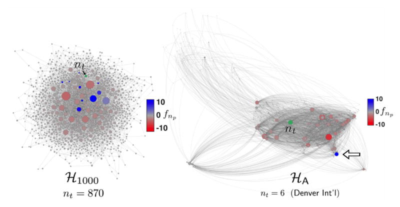
A representative target node (n_t, green) for each network was selected and f-scores for all other nodes were computed and shown by colorscale. Node widths reflect total edge weight including self-loops for each node, and the spatial arrangement results from the Gephi Force Atlas algorithm [69] (left), or geographical location (right). Edge weights are not depicted. (Right) Most major airports are densely connected throughout the network and by their presence retard average transit times of a random walk to n_t, Denver International Airport. One major airport, Miami’s (white arrow), however, has a substantial positive f-score, meaning average MFPTs to Denver would in fact drop by 10.3% if MIA were removed from the network (c.f. Ref. 71). F-score ranges were −3.8 to 12.3 (ℋ₁₀₀₀) and −8.0 to 10.3 (ℋ_A).

Convergence for a single representative n_p is illustrated in Fig. 5. Qualitatively, convergence behavior was consistent among all tested networks. We observed that the size of the free eigenspectrum |k_F| decreases quasi-linearly each iteration (Fig. 3B) given a selection threshold τ^* = 0.995, and that f̃ convergence is attained within three iterations for ℋ₅₀₀ and four iterations for ℋ₂₀₀₀ (Fig. 3C). The free eigenpairs were distributed throughout the spectra, consistent with our claim that changes in trapping time cannot be fully recovered by extreme eigen-pairs alone (Fig. 5C). Some pairs remain free through several iterations, but only free eigenpairs can remain free and once locked an eigenpair will not be updated further.

Figure 5. Procedure visualization for n_t = 498, n_p = 438 ∈ ℋ₅₀₀ over three iterations.

(A) Pre-procedure eigenvalue error, λ_p – λ₀. (B) F-score estimate f̃, black (open circles). True value, f, shown as dashed blue line. (C) Eigenvector update ΔU (Eq. 9 and appendix line 16); rows are nodes (n), columns are eigenindices (k). Black squares positioned along the top horizontal axis of ΔU indicate free eigenindices k_F (Eq. 13). (D) Magnitudes of eigenvector update displayed at each node n, ||ΔU_[n,1:N]||₂. Only a subset of ℋ₅₀₀ is shown to illustrate changes in relative update magnitude. Target node n_t = 498, green; perturbed node n_p = 438, black (indicated by arrow). The magnitude of the updates decreases approximately two orders of magnitude each iteration. (E) Error of predicted eigenvalues (λ̃ – λ_p) after one iteration, shown using the same axes as in (A). Eigenvalue predictions are only updated once (Eq. 8). (F) Aggregate runtime.

Even though |k_F| apparently decreases, it is not the case that estimated f-scores likewise converge monotonically toward the true f_np, and in fact they often get worse during the first iteration, iter = 0 (Figs. 3C and 5B). That is, a single iteration of eigenvector update (Eq. 9) often produces worse f predictions than scores estimated with only approximated eigenvalues (Fig. 3C, dashed lines). This illustrates that transit/trapping times are many-toone indirect functions of the spectrum; the objective formally being minimized in Eq. 9 (and pseudocode line 16) is not f̃ but the gradient of the Rayleigh quotient (at nodes n_F). Consequently, as free eigenpairs adjust to the graph structure in ℋ_p our estimates f̃ can temporarily suffer. However, as k_F diminishes and trapping time contributions (τ̄^k) stabilize the predicted f-score f̃ generally approaches the true value (Fig. 3C). A final prediction error |f – f̃_iter>0| worse than starting prediction error |f – f̃_iter=0| suggests either a failed k_F selection heuristic (pseudocode lines 4–8) or overly permissive convergence thresholds f^* and τ^*.

When altering a physical network such that n_t trapping times are impacted, f-score accuracy rather than eigenvector convergence is the more relevant statistic. While f-scores are often close to zero for nodes distant from n_t, nodes that are first and second degree neighbors of n_t often have appreciable f_np values, up to 10% for the networks tested (Fig. 4). Figure 6 compares predicted and exact f_np values for neighbor nodes and randomly-selected non-neighbor nodes of n_t = 498 ∈ ℋ₅₀₀. In the upper panels, direct neighbors of n_t are designated with diamonds while foreigners are filled circles. F-scores predicted using the full procedure are denoted f̃^{λ̃, Ũ} (Fig. 6A), whereas those predicted using only updated eigenvalues are denoted f̃^λ̃, ^Ũ₀ (Fig. 6B). As is apparent from the low correlation in panel B, both λ and U must be estimated in response to node removal if we want to accurately model f-scores for neighbors of n_t. This point should be emphasized because many centrality metrics are based only on perturbing eigenvalues and not eigenvectors [59, 72]. Panels A and B illustrate this point specifically for a single chosen n_t, but panel C shows that this discrepancy is consistent across many target nodes: correlation ρ suffers unless both λ̃ and Ũ are estimated with perturbation theory.

Figure 6. Both perturbed eigenvalues and eigenvectors must be estimated for accurate f-score prediction.

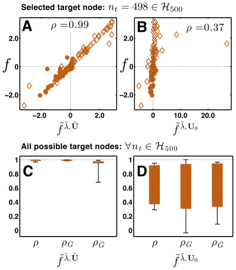
(A) F-score scatter plot for representative target node n_t = 492 in network ℋ₅₀₀. Vertical axis is the exact f-score f, horizontal axis is the predicted f-score f̃, for all nodes n_p ≠ 492 ∈ ℋ₅₀₀. Diamonds denote neighbors of n_t (n_p ∈ G_nt), dots foreigners (n_p ∈ Ḡ_nt). (B) Estimated f-scores f̃ computed from unperturbed eigenvectors U₀ and estimated eigenvalues λ̃; axes as in (A). (C) and (D) The distribution of prediction accuracy for all target nodes in ℋ₅₀₀; f-scores are computed using both perturbed (C) and unperturbed (D) eigenvectors U. A correlation of ρ = 1.0 means perfect prediction accuracy. Accuracy over only neighbors of each n_t is labeled ρ_G, accuracy for foreigners of each n_t is labeled ρ_Ḡ, and correlation over all perturbed nodes is labeled as ρ. Box limits indicate upper and lower quartiles; whiskers show complete data range.

Figure 7 illustrates f-score accuracy and efficiency across the six tested networks. In all panels the horizontal axis gives the relative degree of n_t; this allows us to observe that high correlations (ρ), low normalized root mean squared error (NRMSE), and modest speedup values are all consistent for highly-to-lowly connected target nodes. Each datapoint in Fig. 7B specifically is defined:

$$\text{NRMSE}=\frac{\sqrt{\frac{1}{\mid N_p\mid }{\sum }_{n_p\in N_p}{({\stackrel{\sim }{f}}_{n_p}-f_{n_p})}^2}}{\mid max{f}_{n_p}-min{f}_{n_p}\mid }.$$ (14)

Figure 7. F-score accuracy and efficiency for synthetic and real networks.

Synthetic networks left, real networks right. Horizontal axis in all panels denotes the weighted degree of n_t as a percentage of the maximally-weighted node, $\underset{n_t}{max}{\mathbf{s}}_{n_t\in \mathcal{H}}$. Target nodes n_t were selected by binning all nodes into 20 equal bins according to degree and then randomly selecting 10 target nodes equally spaced across nonempty bins. (A) Accuracy as determined by correlation of predicted f-scores, f̃, with ground truth f-scores, f, denoted ρ. (B) Normalized root mean squared error (Eq. 14). (C) Run-time improvement against direct method, where whiskers show maximum and minimum values. (D) Weighted degree distributions for all nodes n. Colors indicate network selection. See Table II for a summary of these results.

Regarding efficiency, our procedure is about as fast as using brute force matrix inversion for networks with N < 500, but for larger networks we see a consistent algorithmic advantage (Fig. 7C).

A summary of efficiency and accuracy statistics is provided in Table II. Because ground truth f_np values are often near zero, we ask as a control what accuracy is obtainable if λ or U are not updated. Table II therefore provides the average normalized room mean squared error when U is not updated but λ is ( ${\overline{\text{NRMSE}}}_{\stackrel{\sim }{\lambda },{\mathbf{U}}_0}$), and the same statistic is given for when all f̃_np’s are assumed to be zero ( ${\overline{\text{NRMSE}}}_{{\lambda }_0,{\mathbf{U}}_0}$). Again it is clear that both λ and U must be updated to ensure good f_np accuracy.

Table II. Accuracy and efficiency of predicted f-scores.

Algorithm accuracy evaluated with correlation ρ, Spearman rank correlation ρ_s, and root mean squared error normalized by the range of exact scores, $\overline{\text{NRMSE}}$. As controls we also show accuracies for f-score estimates derived without eigenvector updates, ${\overline{\text{NRMSE}}}_{\stackrel{\sim }{\lambda },{\mathbf{U}}_0}$ and those derived from the intact spectrum, ${\overline{\text{NRMSE}}}_{{\lambda }_0,{\mathbf{U}}_0}$ (which equates to f̃_np = 0). The overline indicates weighted average over all tested n_t’s, i.e., over all NRMSE values in Fig. 7B. Some n_p nodes are tested more than once with different target nodes n_t, so total n_p count can exceed the network size.

	Total nt	Total np	ρ	ρs	${\overline{\text{NRMSE}}}_{\stackrel{\sim }{\lambda },\stackrel{\sim }{\mathbf{U}}}$	${\overline{\text{NRMSE}}}_{\stackrel{\sim }{\lambda },{\mathbf{U}}_0}$	${\overline{\text{NRMSE}}}_{{\lambda }_0,{\mathbf{U}}_0}$	Avg. speedup
ℋ500	10	607	0.99	0.98	0.027	0.181	0.192	1.05
ℋ1000	10	837	0.99	0.98	0.026	0.173	0.200	1.82
ℋ2000	10	1880	0.99	0.99	0.021	0.108	0.144	3.38
ℋA	10	880	0.99	0.99	0.012	0.102	0.109	1.28
ℋY ST	10	550	1.00	0.99	0.009	0.174	0.234	4.27
ℋUC	10	1117	0.99	0.97	0.016	0.096	0.127	2.83

CONCLUSIONS

Graph-spectra-derived centrality measures have proven useful for many network modeling tasks [73–76]. At least for Markov-type networks that evolve temporally, we think a concrete interpretation of centrality is provided by the spectral formulation of mean first passage times. Indeed, Eq. 6 formulates squared row vectors of U into a convenient quantity τ̄_nt where we do not need to inspect individual eigenfrequencies in order to assess the topological importance of n_p [22]. That is, individual elements of U_[np,1:N] may ambiguously increase or decrease upon network perturbation, but we can always interpret an f-score to signify that node n_p helps (f_np > 0) or hinders (f_np < 0) graph transitions to n_t. Interestingly, these small changes in transit times manifest themselves in various and discontiguous regions of the Laplacian spectrum (Figs. 3A and 5C), precluding use of many traditional sparse eigensolvers.

However, our primary focus has been to show that, algorithmically, careful selection of eigenpairs k_F can produce a less expensive approximation f̃ that avoids the fundamental matrix Z. This selection cannot be made by comparing the intact and perturbed spectra (since it would require directly computing the latter), but we can guess that nodes with large Rayleigh quotient gradients (Appendix line 5) will reveal eigenpairs that either (1) will move substantially upon node perturbation (k_F) or that (2) will remain stationary (k_L). Iterative application of first-order perturbation theory to both λ̃ and Ũ for only this selected subspace (k_F) then provides an approximate perturbed spectrum faster than dense eigen-decomposition (Fig. 7C).

Because f-scores are usually linear functions of the perturbation magnitude ε ∈ [0, 1], it is not necessary to completely remove node n_p from the graph and problematically decrement the rank of U. Instead, we chose a very small ε so that the eigenvector shifts are small and linear estimates are accurate. This approach has the additional advantage that nodes are never disconnected from the primary graph component when a strict bottleneck node is perturbed. In these situations the f-score cannot fairly be viewed as the change in transit times were n_p to be removed since some paths to n_t would become impossible. The interpretation in these cases should be that f_np represents changes in transit times were n_p to be almost completely removed from the network.

There are many ways of describing what happens to a network when it is damaged or altered [57, 77, 78]. F-scores contribute to this discussion as well because it is sometimes robustness at some target node that is more important than global network stability, and f-scores reveal exactly that. Though many networks in the biological and social sciences surpass in size those considered here, coarse-graining methods [53] can be applied so that the resultant network is amenable to our method.

APPENDIX: Fast f-score estimation

INPUT: Laplacians L and Lp of network ℋ, target node index nt, and perturbed node indices Np
OUTPUT: f̃ (np, nt, ℋ) ∀np ∈ Np.
1:	(U0, λ) ← eig (L)	▷ Direct eigendecomposition
2:	U ← U0
3:	${\overline{\tau }}_{n_t}^k\leftarrow \left(\frac{N}{N-1}\right)\left(\frac{s{u}_{k{n}_t}^2-\left({\mathbf{s}}^T{\mathbf{u}}_k\right)u_{k{n}_t}}{{\lambda }_k}\right)\forall k\ne 1$
Predict free/locked modes, kF, kL, by estimating $\mathrm{\Delta }{\overline{\tau }}_{n_t}^k$
4:	for np ∈ Np do
5:	U[np∪Gnp,2:N] ← U[np∪Gnp,2:N] − ∇r (U[np∪Gnp,2:N])	▷ see main text Eq. 12
6:	Uk = Uk/||Uk||	▷ Normalize all columns of U
7:	$\stackrel{\sim }{\mathrm{\Delta }}{\overline{\tau }}_{n_t}^k\leftarrow \left(\frac{N}{N-1}\right)\left(\frac{s_p{u}_{k{n}_t}^2-({\mathbf{s}}_p^T{\mathbf{u}}_k)u_{k{n}_t}}{{\lambda }_k}\right)-{\overline{\tau }}_{n_t}^k$, ∀k ≠ 1
8:	$k_F\leftarrow \underset{k}{\text{find}}\left(\mid \stackrel{\sim }{\mathrm{\Delta }}{\overline{\tau }}_{n_t}^k\mid >{\overline{\tau }}^{\ast }\right)$, kL ← {2 … N}\kF	▷ Select free/locked eigenpairs
Estimate perturbed eigenvalues
9:	Select ε~ 10−4
10:	U ← U0
11:	${\stackrel{\sim }{\lambda }}_k\leftarrow k+\epsilon \ast \left({({\mathbf{U}}_k{.}^2)}^T{\mathbf{L}}_{n_p}-2{\lambda }_k{u}_{kk}^2\right)\forall k\ne 1$
12:	Generate matrix of update weights: Λij = (λ̃i − λ̃j)−1, Λii = 0, i, j ∈ {2 … N}
Update U iteratively until f̃(np, nt, ℋ) converges
13:	iter ← 0
14:	Store free node indices: nF = {np ∪ ng}	▷ only np and neighborhood eligible for update
15:	while converged == 0 do	▷ Begin iteration for f̃np
16:	$\mathrm{\Delta }{\mathbf{U}}_{[1:N,k_F]}\leftarrow {\mathbf{U}}_{[1:N,k_F]}\left\{{\mathbf{U}}_{[n_F,k_F]}^T\left({\mathbf{L}}_{p[n_F,1:N]}{\mathbf{U}}_{[1:N,k_F]}-{\mathbf{U}}_{[n_F,k_F]}\ast \mathbf{I}{\stackrel{\sim }{\lambda }}_{k_F}\right).\ast {\mathrm{\Lambda }}_{[k_F,k_F]}\right\}$	▷ see Eq. 9
17:	Ũ ← U+ ΔU
18:	${\stackrel{\sim }{\overline{\tau }}}_{n_t}^k\leftarrow \left(\frac{N}{N-1}\right)\left(\frac{s_p{\stackrel{\sim }{u}}_{k{n}_t}^2-({\mathbf{s}}_p^T{\stackrel{\sim }{\mathbf{u}}}_k){\stackrel{\sim }{u}}_{k{n}_t}}{{\stackrel{\sim }{\lambda }}_k}\right)$, ∀k ∈ kF	▷ Compute updated ${\stackrel{\sim }{\overline{\tau }}}_{n_t}^k$
19:	${\stackrel{\sim }{f}}_{\text{iter}}(n_p,n_t)\leftarrow (1/\epsilon )\ast \frac{{\sum }_{k=2}^N{\stackrel{\sim }{\overline{\tau }}}^k{\sum }_{k=2}^N{\overline{\tau }}^k}{{\sum }_{k=2}^N{\overline{\tau }}^k}$	▷ Estimate new fnp
20:	converged ←|f̃ iter − f̃iter−1|/|f̃iter−1| < f*
21:	if !converged then
22:	$k_F\leftarrow \text{find}\left(\mid \stackrel{\sim }{\mathrm{\Delta }}{\overline{\tau }}_{n_t}^{k_F}\mid >{\overline{\tau }}^{\ast }\right)$
23:	nF ← {1 … N}	▷ All nodes now eligible for update
24:	U ← Ũ
25:	iter ← iter + 1
26:	end if
27:	end while
28:	end for

References

- 1.Colizza Vittoria, Barrat Alain, Barthélemy Marc, Vespignani Alessandro. The role of the airline transportation network in the prediction and predictability of global epidemics. Proceedings of the National Academy of Sciences of the United States of America. 2006;103:2015–2020. doi: 10.1073/pnas.0510525103. [DOI] [PMC free article] [PubMed] [Google Scholar]
- 2.Colizza Vittoria, Pastor-Satorras Romualdo, Vespignani Alessandro. Reaction–diffusion processes and metapopulation models in heterogeneous networks. Nature Physics. 2007;3:276–282. [Google Scholar]
- 3.Memmott J, Waser NM, Price MV. Tolerance of pollination networks to species extinctions. Proceedings of the Royal Society B: Biological Sciences. 2004;271:2605–2611. doi: 10.1098/rspb.2004.2909. [DOI] [PMC free article] [PubMed] [Google Scholar]
- 4.Kitsak Maksim, Gallos Lazaros K, Havlin Shlomo, Liljeros Fredrik, Muchnik Lev, Eugene Stanley H, Makse Hernán A. Identification of influential spreaders in complex networks. Nature Physics. 2010;6:888–893. [Google Scholar]
- 5.Barahona Mauricio, Pecora Louis M. Synchronization in small-world systems. Physical Review Letters. 2002;89:054101. doi: 10.1103/PhysRevLett.89.054101. [DOI] [PubMed] [Google Scholar]
- 6.Albert Réka, Barabasi Albert-Laszlo. Statistical mechanics of complex networks. Reviews of modern physics. 2002;74:47. [Google Scholar]
- 7.Van Mieghem Piet. Epidemic phase transition of the SIS type in networks. EPL (Europhysics Letters) 2012;97:48004. [Google Scholar]
- 8.Bullmore Ed, Sporns Olaf. Complex brain networks: graph theoretical analysis of structural and functional systems. Nature Reviews Neuroscience. 2009;10:186–198. doi: 10.1038/nrn2575. [DOI] [PubMed] [Google Scholar]
- 9.Lawniczak AT, Gerisch A, Maxie K. Effects of randomly added links on a phase transition in data network traffic models. Proc of the 3rd International DCDIS Conference. 2003 [Google Scholar]
- 10.Chodera John D, Pande Vijay S. The social network (of protein conformations) Proceedings of the National Academy of Sciences of the United States of America. 2011;108:12969–12970. doi: 10.1073/pnas.1109571108. [DOI] [PMC free article] [PubMed] [Google Scholar]
- 11.Pagani Giuliano Andrea, Aiello Marco. The Power Grid as a complex network: A survey. Physica A: Statistical Mechanics and its Applications. 2013;392:2688–2700. [Google Scholar]
- 12.Watts DJ, Strogatz SH. Collective dynamics of ‘small-world’ networks. Nature. 1998;393:440–442. doi: 10.1038/30918. [DOI] [PubMed] [Google Scholar]
- 13.Prakash BA, Vreeken J, Faloutsos C. Efficiently spotting the starting points of an epidemic in a large graph. Knowledge and information systems. 2014 [Google Scholar]
- 14.Barrat Alain, Barthélemy Marc, Vespignani Alessandro. Dynamical Processes on Complex Networks. Cambridge University Press; 2008. [Google Scholar]
- 15.Wang Hui, Huang Jinyuan, Xu Xiaomin, Xiao Yanghua. Damage attack on complex networks. Physica A: Statistical Mechanics and its Applications. 2014:1–15. [Google Scholar]
- 16.Gutiérrez Ricardo, Sendiña-Nadal Irene, Zanin Massimiliano, Papo David, Boccaletti Stefano. Targeting the dynamics of complex networks. Scientific Reports. 2012;2:396–396. doi: 10.1038/srep00396. [DOI] [PMC free article] [PubMed] [Google Scholar]
- 17.Soundararajan Venky, Aravamudan Murali. Global connectivity of hub residues in Oncoprotein structures encodes genetic factors dictating personalized drug response to targeted Cancer therapy. Scientific Reports. 2014;4:7294. doi: 10.1038/srep07294. [DOI] [PMC free article] [PubMed] [Google Scholar]
- 18.Benzi Michele, Klymko Christine. A matrix analysis of different centrality measures. 2013 arXiv preprint arXiv:1312.6722. [Google Scholar]
- 19.Bounova Gergana, de Weck Olivier. Overview of metrics and their correlation patterns for multiple-metric topology analysis on heterogeneous graph ensembles. Physical Review E. 2012;85:016117. doi: 10.1103/PhysRevE.85.016117. [DOI] [PubMed] [Google Scholar]
- 20.Brush Eleanor R, Krakauer David C, Flack Jessica C. A Family of Algorithms for Computing Consensus about Node State from Network Data. PLoS computational biology. 2013;9:e1003109. doi: 10.1371/journal.pcbi.1003109. [DOI] [PMC free article] [PubMed] [Google Scholar]
- 21.da Costa LF, Rodrigues FA, Travieso G, Villas Boas PR. Characterization of complex networks: A survey of measurements. Advances in Physics. 2007;56:167–242. [Google Scholar]
- 22.Van Mieghem Piet. Graph eigenvectors, fundamental weights and centrality metrics for nodes in networks. 2014 arXiv preprint arXiv:1401.4580. [Google Scholar]
- 23.Bowman Gregory R, Pande Vijay S. Protein folded states are kinetic hubs. Proceedings of the National Academy of Sciences of the United States of America. 2010;107:10890–10895. doi: 10.1073/pnas.1003962107. [DOI] [PMC free article] [PubMed] [Google Scholar]
- 24.Dickson Alex, Brooks Charles., III Quantifying hub-like behavior in protein folding networks. Journal of Chemical Theory and Computation. 2012;8:3044–3052. doi: 10.1021/ct300537s. [DOI] [PMC free article] [PubMed] [Google Scholar]
- 25.Dickson Alex, Brooks Charles., III Native States of Fast-Folding Proteins Are Kinetic Traps. Journal of the American Chemical Society. 2013;135:4729–4734. doi: 10.1021/ja311077u. [DOI] [PMC free article] [PubMed] [Google Scholar]
- 26.Liu Hongxiao, Zhang Zhongzhi. Laplacian spectra of recursive treelike small-world polymer networks: Analytical solutions and applications. The Journal of Chemical Physics. 2013;138:114904. doi: 10.1063/1.4794921. [DOI] [PubMed] [Google Scholar]
- 27.Aditya Prakash B, Vreeken Jilles, Faloutsos Christos. Spotting culprits in epidemics: How many and which ones? IEEE International Conference on Data Mining. 2012;12:11–20. [Google Scholar]
- 28.McGraw Patrick N, Menzinger Michael. Laplacian spectra as a diagnostic tool for network structure and dynamics. Physical Review E. 2008;77:031102. doi: 10.1103/PhysRevE.77.031102. [DOI] [PubMed] [Google Scholar]
- 29.Pauls Scott D, Remondini Daniel. Measures of centrality based on the spectrum of the Laplacian. Physical Review E. 2012;85:066127. doi: 10.1103/PhysRevE.85.066127. [DOI] [PubMed] [Google Scholar]
- 30.Yadav Gitanjali, Babu Suresh. NEXCADE: Perturbation Analysis for Complex Networks. PLoS ONE. 2012;7:e41827. doi: 10.1371/journal.pone.0041827. [DOI] [PMC free article] [PubMed] [Google Scholar]
- 31.Ng Andrew Y, Zheng Alice X, Jordan Michael I. Link analysis, eigenvectors and stability. International Joint Conference on Artificial Intelligence. 2001;17:903–910. [Google Scholar]
- 32.Ghoshal Gourab, Barabasi Albert-Laszlo. Ranking stability and super-stable nodes in complex networks. Nature Communications. 2011;2:392–7. doi: 10.1038/ncomms1396. [DOI] [PubMed] [Google Scholar]
- 33.Estrada Ernesto, Rodríguez-Velázquez Juan. Subgraph centrality in complex networks. Physical Review E. 2005;71:056103. doi: 10.1103/PhysRevE.71.056103. [DOI] [PubMed] [Google Scholar]
- 34.Estrada Ernesto, Hatano Naomichi, Benzi Michele. The physics of communicability in complex networks. Physics Reports. 2012;514:89–119. [Google Scholar]
- 35.Chen Juan, Lu Junan, Zhan Choujun, Chen Guanrong. Handbook of Optimization in Complex Networks. Springer; 2012. Laplacian spectra and synchronization processes on complex networks; pp. 81–113. [Google Scholar]
- 36.Monasson Remi. Diffusion, localization and dispersion relations on “small-world” lattices. The European Physical Journal B-Condensed Matter and Complex Systems. 1999;12:555–567. [Google Scholar]
- 37.Li C, Wang H, de Haan W, Stam CJ, Van Mieghem Piet. The correlation of metrics in complex networks with applications in functional brain networks. Journal of Statistical Mechanics: Theory and Experiment. 2011;2011:P11018. [Google Scholar]
- 38.Savol Andrej, Chennubhotla Chakra S. Quantifying the Sources of Kinetic Frustration in Folding Simulations of Small Proteins. Journal of Chemical Theory and Computation. 2014;10:2964–2974. doi: 10.1021/ct500361w. [DOI] [PMC free article] [PubMed] [Google Scholar]
- 39.Zhang Zhongzhi, Julaiti Alafate, Hou Baoyu, Zhang Hongjuan, Chen Guanrong. Mean first-passage time for random walks on undirected networks. The European Physical Journal B. 2011;84:691–697. [Google Scholar]
- 40.Doyle Peter G, Snell James Laurie. Carus Monographs. Mathematical Association of America; Washington: 1984. Random Walks and Electric Networks. [Google Scholar]
- 41.Kemeny JG, Snell James Laurie. Finite Markov Chains. Springer Verlag; New York: 1976. [Google Scholar]
- 42.Shanahan Murray. Metastable chimera states in community-structured oscillator networks. Chaos. 2010;20:013108–013108. doi: 10.1063/1.3305451. [DOI] [PubMed] [Google Scholar]
- 43.Villegas Pablo, Moretti Paolo, Muñoz Miguel A. Frustrated hierarchical synchronization and emergent complexity in the human connectome network. Scientific Reports. 2014;4:5990–5990. doi: 10.1038/srep05990. [DOI] [PMC free article] [PubMed] [Google Scholar]
- 44.von Luxburg Ulrike, Radl Agnes, Hein Matthias. Hitting and commute times in large graphs are often misleading. 2010 arXiv preprint arXiv:1003.1266. [Google Scholar]
- 45.von Luxburg Ulrike, Radl Agnes, Hein Matthias. Getting lost in space: Large sample analysis of the commute distance. Advances in Neural Information Processing Systems. 2010;23:2622–2630. [Google Scholar]
- 46.Newman MEJ. Audio and Electroacoustics Newsletter. IEEE; 2004. Power laws, Pareto distributions and Zipf’s law. [DOI] [Google Scholar]
- 47.Kiemer Lars, Costa Stefano, Ueffing Marius, Cesareni Gianni. WI-PHI: A weighted yeast interactome enriched for direct physical interactions. Proteomics. 2007;7:932–943. doi: 10.1002/pmic.200600448. [DOI] [PubMed] [Google Scholar]
- 48.Panzarasa Pietro, Opsahl Tore, Carley Kathleen M. Patterns and Dynamics of Users’ Behavior and Interaction: Network Analysis of an Online Community. Journal of the American Society for Information Science and Technology. 2009;60:911–932. [Google Scholar]
- 49.Lovász László. Random walks on graphs: A survey. Combinatorics, Paul erdos is eighty. 1993;2:1–46. [Google Scholar]
- 50.von Luxburg Ulrike. A tutorial on spectral clustering. Statistics and Computing. 2007;17:395–416. [Google Scholar]
- 51.Hager William. Updating the inverse of a matrix. SIAM review. 1989:221–2339. [Google Scholar]
- 52.Lin Yuan, Zhang Zhongzhi. Random walks in weighted networks with a perfect trap: An application of Laplacian spectra. Physical Review E. 2013;87:062140. doi: 10.1103/PhysRevE.87.062140. [DOI] [PubMed] [Google Scholar]
- 53.Gfeller David, De Los Rios Paolo. Spectral coarse graining and synchronization in oscillator networks. Physical Review Letters. 2008;100:174104–174104. doi: 10.1103/PhysRevLett.100.174104. [DOI] [PubMed] [Google Scholar]
- 54.Lafon Stéphane S, Lee Ann BAB. Diffusion maps and coarse-graining: A unified framework for dimensionality reduction, graph partitioning, and data set parameterization. IEEE Transactions on Pattern Analysis and Machine Intelligence. 2006;28:1393–1403. doi: 10.1109/TPAMI.2006.184. [DOI] [PubMed] [Google Scholar]
- 55.Krishnan Dilip, Fattal Raanan, Szeliski Richard. Efficient preconditioning of laplacian matrices for computer graphics. ACM Transactions on Graphics. 2013;32:1. [Google Scholar]
- 56.Qi X, Fuller E, Wu Q, Wu Y, Zhang CQ. Laplacian centrality: A new centrality measure for weighted networks. Information Sciences. 2012 doi: 10.1016/j.ins.2011.12.027. [DOI] [Google Scholar]
- 57.Van Mieghem Piet, Stevanović Dragan, Kuipers Fernando, Li Cong, van de Bovenkamp Ruud, Liu Daijie, Wang Huijuan. Decreasing the spectral radius of a graph by link removals. Physical Review E. 2011;84:016101. doi: 10.1103/PhysRevE.84.016101. [DOI] [PubMed] [Google Scholar]
- 58.Kalloniatis Alexander C. From incoherence to synchronicity in the network Kuramoto model. Physical Review E. 2010;82:066202–066202. doi: 10.1103/PhysRevE.82.066202. [DOI] [PubMed] [Google Scholar]
- 59.Milanese Attilio, Sun Jie, Nishikawa Takashi. Approximating spectral impact of structural perturbations in large networks. Physical Review E. 2010;81:046112. doi: 10.1103/PhysRevE.81.046112. [DOI] [PubMed] [Google Scholar]
- 60.Butler Steve. Interlacing for weighted graphs using the normalized Laplacian. Electronic Journal of Linear Algebra. 2007;16:87. [Google Scholar]
- 61.Abiad Aida, Fiol Miquel A, Haemers Willem H, Perarnau Guillem. An interlacing approach for bounding the sum of Laplacian eigenvalues of graphs. Linear Algebra and its Applications. 2014;448:11–21. [Google Scholar]
- 62.Wu Baofeng, Shao Jiayu, Yuan Xiying. Deleting vertices and interlacing Laplacian eigenvalues. Chinese Annals of Mathematics, Series B. 2010;31:231–236. [Google Scholar]
- 63.Wilkinson JH. The algebraic eigenvalue problem. Oxford University Press; 1965. [Google Scholar]
- 64.Liu XL, Oliveira CS. Iterative modal perturbation and reanalysis of eigenvalue problem. Communications in Numerical Methods in Engineering. 2003;19:263–274. [Google Scholar]
- 65.MacKay David. Information theory, inference, and learning algorithms. Cambridge University Press; 2003. [Google Scholar]
- 66.Hernandez V, Roman JE, Tomas A, Vidal V. Arnoldi methods in SLEPc. SLEPc Technical Report STR-4. 2007 [Google Scholar]
- 67.Trefethen Loyd, Bau David. Numerical Linear Algebra. SIAM; Philadelphia: 1997. [Google Scholar]
- 68.MATLAB, version 7.14.0.739 (R2012a) The Math-Works Inc; Natick, Massachusetts: [Google Scholar]
- 69.Bastian Mathieu, Heymann Sebastien, Jacomy Mathieu. Gephi: an open source software for exploring and manipulating networks. ICWSM. 2009:361–362. [Google Scholar]
- 70.Muchnik Lev. Complex Networks Package for MatLab (Version 1.6) ( www.levmuchnik.net)
- 71.Verma T, Araújo NAM, Herrmann Hans J. Revealing the structure of the world airline network. Scientific Reports. 2014;4 doi: 10.1038/srep05638. [DOI] [PMC free article] [PubMed] [Google Scholar]
- 72.Restrepo Juan G, Ott Edward, Hunt Brian R. Characterizing the dynamical importance of network nodes and links. Physical Review Letters. 2006;97:094102. doi: 10.1103/PhysRevLett.97.094102. [DOI] [PubMed] [Google Scholar]
- 73.Boccaletti Stefano, Latora V, Moreno Y, Chavez M. Complex networks: Structure and dynamics. Physics reports. 2006 [Google Scholar]
- 74.Cvetković Dragoš, Rowlinson Peter, Simić Slobodan. An Introduction to the Theory of Graph Spectra. Cambridge University Press; 2009. [Google Scholar]
- 75.Estrada Ernesto, Hatano Naomichi. A vibrational approach to node centrality and vulnerability in complex networks. Physica A: Statistical Mechanics and its Applications. 2010;389:3648–3660. [Google Scholar]
- 76.Schaub MT, Lehmann J, Yaliraki SN. Structure of complex networks: Quantifying edge-to-edge relations by failure-induced flow redistribution. Network Science. 2014;2:66–89. [Google Scholar]
- 77.Liu D, Wang H, Van Mieghem Piet. Spectral perturbation and reconstructability of complex networks. Physical Review E. 2010;81:016101. doi: 10.1103/PhysRevE.81.016101. [DOI] [PubMed] [Google Scholar]
- 78.Estrada Ernesto, Vargas-Estrada Eusebio, Ando Hiroyasu. Communicability Angles Reveal Critical Edges for Network Consensus Dynamics. 2015 doi: 10.1103/PhysRevE.92.052809. ArXiv e-prints. [DOI] [PubMed] [Google Scholar]