Improved MRI Thermometry with Multiple-Echo Spirals

Abstract

Purpose

Low-bandwidth PRF shift thermometry is used to guide HIFU ablation treatments. Low sampling bandwidth is needed for high SNR with short acquisition times, but can lead to off-resonance artifacts. In this work, improved multiple-echo thermometry is presented that allows for high bandwidth and reduced artifacts. It is also demonstrated with spiral sampling, to improve the trade-off between resolution, speed, and measurement precision.

Methods

Four multiple-echo thermometry sequences were tested in vivo, one using 2DFT sampling and three using spirals. The spiral sequences were individually optimized for resolution, for speed, and for precision. Multi-frequency reconstruction was used to correct for off-resonance spiral artifacts. Additionally, two different multi-echo temperature reconstructions were compared.

Results

Weighted combination of per-echo phase differences gave significantly better precision than least squares off-resonance estimation. Multiple-echo 2DFT sequence obtained precision similar to single-echo 2DFT, while greatly increasing sampling bandwidth. The multi-echo spiral acquisitions achieved 2× better resolution, 2.9× better uncertainty, or 3.4× faster acquisition time, without negatively impacting the other two design parameters as compared to single-echo 2DFT.

Conclusion

Multi-echo spiral thermometry greatly improves the capabilities of temperature monitoring, and could improve transcranial treatment monitoring capabilities.

Introduction

MR-guided focused ultrasound (MRgFUS) treatments are being used for non-invasive or minimally invasive treatment in an increasing number of interventions. By focusing ultrasound energy to a spot within the body, HIFU is able to ablate targets within the body without surgical incision. Transcranial HIFU can ablate targets deep within the brain, and is being used to treat essential tremor (1), neuropathic pain (2,3), and brain tumors (4). During these treatments, MRI thermometry is used to monitor the treatment, by ensuring accurate targeting of the heating, by measuring the thermal dose delivered to the target, and by monitoring non-targeted areas of the brain to ensure that no undesired heating occurs.

Accurate treatment monitoring requires temperature monitoring with high resolution, fast acquisition speed, and good measurement precision. PRF shift thermometry is the preferred approach for this temperature imaging (5,6), as temperature maps with sufficient precision can be acquired in seconds. Individual sonications during treatment may be as short as 10 seconds, and treatments can generate lesions that are approximately 3-4mm in diameter and 4-5mm tall (3). Therefore, acquisitions must be 5 seconds or faster to ensure multiple measurements of any sonication, and resolution must be at least 1-2 mm in-plane resolution with 3 mm or thinner slice thickness to accurately measure focal temperature (7). Improvements in the speed, precision, resolution, or volume coverage of MR thermometry would improve the safety and quality of MR-guided HIFU, by improving the ability of the clinician to monitor treatment.

Temperature SNR (tSNR) in PRF shift thermometry depends on the ability of a sequence to measure temperature-induced changes in frequency (B₀). Therefore, temperature SNR increases linearly with TE (due to accrued phase) for a fixed magnitude SNR (8). Because tSNR depends on both the measured change in temperature and on the noise in the measurement, this paper will often refer only to the uncertainty in the temperature measurement, which is independent of temperature rise. With limited time available for fast imaging, maximum TE and TR are limited when using a large number of phase encodes, resulting in sub-optimal SNR due to TE<T₂*, though TE can be increased through echo shifting (9) or by using non-Cartesian trajectories (8,10–13).

During transcranial MRgFUS, the ultrasound hardware surrounds the head and does not leave room for traditional MR head coils. This restricts current transcranial thermometry to the use of the MRI body coil for imaging, which yields significantly lower SNR than is achievable using standard brain imaging hardware. Additionally, because the body coil is single channel, parallel imaging (14) or similar techniques that require multiple receiver channels are not compatible with current treatment monitoring. Therefore, all testing and validation in this work was performed with a body coil.

To maximize temperature precision for standard 2DFT thermometry, all available time in a TR is typically used for sampling. This results in long readouts that are sensitive to off-resonance, and will result in geometric distortions in the presence of off-resonance. One approach to reducing off-resonance sensitivity while maintaining SNR is by collecting multiple echoes. This has been demonstrated previously using 2DFT (15,16), in lipids (9,17,18) or by using multiple magnetization pathways (19). In earlier multi-echo 2DFT work (15), temperature was estimated by performing a linear fit of the phase vs echo times, and determining the slope. A tSNR-optimal approach for combining multiple independent temperature estimates was derived in (19), which can be used to perform tSNR-optimal echo combination in the multiple-echo 2DFT sequence, and which was used in more recent work (16). However, a comparison of the temperature uncertainties obtained with the two reconstruction approaches was not presented with the improved approach, so one has been included in this work.

Using non-Cartesian trajectories, such as EPI or spiral, can reduce the number of TRs necessary to acquire a particular resolution, as compared to 2DFT. However, these trajectories are more sensitive to off-resonance and other imperfections, and can cause severe artifacts. Off-resonance in a 2DFT readout will add affine phase accrual across k-space, causing geometric shifts along the readout dimension and possibly signal pile-up. Off-resonance in EPI readouts also results in geometric distortions, but the artifacts occur in both dimensions. Off-resonance in a spiral readout will add parabolic phase accrual across k-space, altering the point spread function and potentially introducing severe image artifacts (20–22). However, these effects can be minimized by reducing the duration of readouts and/or by applying multi-frequency reconstruction to reduce the amount of off-resonance observed by each voxel (23,24). Multi-frequency reconstructions add computational complexity, though post-gridding correction is significantly faster than pre-gridding correction. These reconstructions also require an estimate of off-resonance, which can either be estimated from low-frequency data (25) or through additional scanning. If residual off-resonance is small, and spiral readouts are short, the spiral-sampling point spread function can be restored. While EPI trajectories offer similar imaging efficiency to spiral, the lack of geometric shift artifacts in spiral are advantageous for thermometry. The geometric shifts induced by off-resonance in EPI readouts (or with traditional 2DFT) can cause misregistration between heating and anatomical targeting. Additionally, calculation of off-resonance maps from spiral data is more straightforward, as the voxel locations (and associated off-resonance) do not change depending on reconstruction frequency. Use of a spiral-in trajectory places the effective echo time at the end of the readout duration, as opposed to the center for 2DFT or EPI readouts, which will often increase temperature measurement precision. For these reasons, spiral readouts were chosen for this work.

The purpose of this work was to develop and test multi-echo spiral thermometry sequences, to explore the improved performance they offer and to establish the feasibility of both the sequences and of their reconstruction and post-processing. Multi-echo spiral sequences were designed to improve different aspects of thermometry performance (speed, precision, resolution) and were compared to single- and multi-echo 2DFT thermometry. Two temperature reconstruction approaches for multi-echo thermometry were compared to illustrate the importance of proper reconstruction. Post-gridding multi-frequency correction was used to reconstruct the multi-echo spiral data, using off-resonance maps calculated directly from the data, and were shown to correct for off-resonance spiral artifacts. Measurement precision for each sequence was measured in vivo without heating on several volunteers. Finally, each sequence was used to monitor temperature while heating a phantom, to ensure that the sequences worked properly while imaging focal heating.

Methods

Five variations of spoiled gradient echo thermometry sequences were designed, to compare performance of conventional 2DFT thermometry, multiple-echo 2DFT thermometry, and multi-echo spiral thermometry. All sequences were designed using MATLAB (Natick, MA) and SpinBench (HeartVista, Inc. Menlo Park, CA), and implemented on a GE 3T Signa MR scanner using RTHawk (HeartVista, Inc. Menlo Park, CA USA). The first sequence (“2DFT”) was a single-echo 2DFT SPGR sequence meant to mimic the temperature sequence currently used to monitor brain treatments. The second sequence (“ME2DFT”) was a multiple-echo 2DFT SPGR sequence, without flyback. The remaining three sequences also used multiple echoes, but with spiral k-space trajectories. Alternating echoes were collected with opposing spirals, (to negate potential errors from imperfect gradients.) The design objectives for the three sequences were to optimize speed (“ME_Fast”), resolution (“ME_HighRes”), or temperature uncertainty (“ME_Precise”) without worsening the other two design objectives. Sequence parameters are included in Table 1. For the ME_Fast and ME_HighRes sequences, four spiral readouts were used per TR, with the number of interleaves, resolution, and sampling bandwidth chosen to fit within the specified design constraints. For the ME_Precise sequence, a lower sampling bandwidth was chosen for increased SNR. This improved SNR allowed for longer echo times to be measured with sufficient remaining signal, and a total of six spiral readouts were used. For each spiral sequence, duration of each readout was restricted to ≤9.25 ms, which ensures ≤π/2 intra-readout phase accrual (preserving the desired impulse response and resolution) for off-resonance of ≤27 Hz. For the heating experiments in phantom, a 20° flip angle was used for each sequence. For in vivo measurements, optimal flip angles were determined for each sequence, as described in the following section.

Table 1. Sequence parameters for the 5 implemented thermometry sequences.

	2DFT	ME2DFT	ME_Fast	ME_HighRes	ME_Precise
Resolution (mm)	1.09 × 2.19	1.09 × 2.19	1.49 × 1.49	1.09 × 1.09	1.49 × 1.49
Sequence Time	3.64 sec	3.48 sec	1.08 sec	3.65 sec	3.55 sec
TR (ms)	28.4	27.2	44.8	45.1	64.5
# Interleaves	128	128	24	81	55
TEs (ms)	14.2	5.2, 7.5, 9.7, 12.0, 14.2, 16.5, 18.8, 21.0, 23.3	12.7, 22.6, 32.6, 42.5	12.8, 22.8, 32.8, 42.8	12.7, 22.5, 32.5, 42.4, 52.3, 62.2
Flip Angle: phantom	20°	20°	20°	20°	20°
Flip Angle: in vivo	11°	10°	12°	11°	14°
RO Duration (ms)	22.53	2.048	9.25	9.24	9.24
Sampling Bandwidth (kHz)	11.36	125	125	71.43	55.56
Slice Thickness	3 mm	3 mm	3 mm	3 mm	3 mm

Optimal Flip Angle Measurement

To estimate the best flip angle for each sequence, a healthy volunteer was scanned while stepping through flip angles for each sequence. All volunteers in this study were scanned under IRB approval, with informed consent. Three image frames were acquired at each flip angle, with the first frame of each flip angle discarded to ensure steady-state. Each scan began with a 21° flip, decreasing in increments of 1° down to 1°. Relative SNR across flip angles for each sequence was calculated in post-processing as follows: Average images were determined by averaging across all acquired images across flip angles, and the conjugate phase of these average images were applied to each individual image to rotate the images into the real plane. The average real signal was calculated within a large ROI for each image. These average signals were multiplied by their corresponding echo time to simulate temperature uncertainty, and multiple echoes were combined using sum-of-squares. Finally, each sequence's measured signal levels were divided by the maximum observed, to obtain normalized relative SNR.

Temperature SNR Data Collection

To evaluate temperature uncertainty in vivo, three healthy volunteers were scanned with each of the five sequences. For each sequence, the optimal flip angle determined in the previous experiment was utilized (as listed in Table 1). Each volunteer was scanned using the body coil, at an axial slice located above the eyebrows, and were instructed to remain still (using no other restraint). Higher-order shims were used to minimize B₀ variation across the full brain prior to scanning. At least 23 frames of each sequence were acquired. The first frame was discarded to ensure steady-state, and the next four frames were averaged to provide a baseline. The remaining frames were used for analysis. For each spiral sequence, an additional “delayed baseline” was collected prior to acquisition of the baseline and analysis data. In the delayed baseline, 2 ms of dead time was inserted between excitation and the first readout, to delay each TE by 2 ms. These delayed baselines were used for multi-frequency reconstruction. To assess the effectiveness of multi-frequency reconstruction, an additional volunteer was scanned at a more inferior axial plane in a region of greater off-resonance variation, which was not included in the temperature SNR comparisons.

Phantom Heating Experiment

Each sequence was also used to measure temperature while heating a focal spot in a HIFU phantom, to assess temperature accuracy and temperature image quality in the presence of heating. Each sequence used a flip angle of 20° for this experiment. Heating was performed using the Exablate 2000 system (Insightec, Haifa, Israel) with 5 separate sonications, one per sequence. The imaging slice was located at the ultrasound focus (set to 12.3 cm from the transducer), and each sonication was 30 sec long with 32.4 W acoustic power. The order of the acquisitions was: ME_Fast, ME_Precise, ME_HighRes, ME2DFT, 2DFT. The phantom was allowed to cool for at least 10 minutes between each sonication. Imaging had to be paused briefly to start each sonication, (due to a software limitation in the experimental setup that does not permit sonication onset while the MR scanner is active,) so steady-state was interrupted for that image. The sonication onset time was estimated during post-processing based on the heating time courses. For each sequence, the four frames immediately preceding sonication were averaged to provide a baseline for calculating temperature differences.

Multi-Frequency Reconstruction of Multi-Echo Spiral Data

Multi-frequency reconstruction was performed on all multi-echo spiral sequences, to reduce the effects of off-resonance on image quality. For the in vivo data, off-resonance was estimated by converting the phase difference between the baseline and delayed baseline to off-resonance frequency. Different echoes of off-resonance estimates were combined with a weighted average, using baseline magnitude for weighting. For the phantom data, phase accrual across baseline echoes was used to estimate off-resonance, as the maximal off-resonance was small enough to avoid aliasing. To perform the multi-frequency reconstruction, k-space position as a function of time was computed using the spiral trajectory. Reconstruction was performed every 10 Hz, across the range of frequencies observed in the off-resonance map. For each off-resonance value, the expected absolute phase for each point in k-space for that frequency was calculated for each TE, and the conjugate of that expected phase was applied to the k-space data. Each voxel then used the result from the closest reconstructed frequency for its final reconstruction.

During ablative FUS treatment, temperature elevations of approximately 22°C are typically created (2). This temperature difference creates a frequency shift of -28 Hz for 3T MRI. To minimize maximal off-resonance in reconstruction, two methods can be used. The first approach would be estimating off-resonance for every frame individually, and using that estimate for multi-frequency reconstruction. The second and simpler approach, used in this work, is to reconstruct all data at the original estimated off-resonance frequency (measured from the baseline) with a +14 Hz offset. For unheated voxels, off-resonance is then +14 Hz, plus the difference between the desired frequency and the closest reconstructed frequency (-5 Hz to +5 Hz for reconstruction every 10 Hz), plus drift of the magnetic field over time. During heating, the frequency will shift from +14 Hz (plus reconstruction offset and drift) to -14 Hz. Therefore, maximal off-resonance of ±19 Hz is expected with this reconstruction approach, generating ≲π/3 phase accrual over the 9.25 ms readout duration.

tSNR-Optimal Weighted Echo Combination

For most of the analysis in this work, temperature changes were calculated using tSNR-optimal weighted echo combination. Temperature changes were calculated independently for each echo of each frame of data, by finding the phase difference between that image and the corresponding baseline. Phase difference was converted to temperature difference assuming α = -0.01 ppm/°C. For each frame of data, B₀ drift was estimated by taking a weighted average of temperature (which corresponds to frequency change), using the baseline magnitudes for relative weighting, and the resulting drift-induced temperature estimate was subtracted from all voxels. Relative tSNR across echoes was estimated on a voxel-wise basis as the product of baseline magnitude and TE. All echoes' temperature estimates were combined into a single estimate using the square of relative tSNR as relative weights, following the tSNR-optimal echo combination approach proposed in (19). Temperature uncertainty was calculated as the standard deviation of measured temperature over time, and average uncertainties were calculated as the spatial mean within a large ROI within the brain. An estimate of efficiency was calculated for each sequence, reflecting the relative tSNR available for the sequence. Sequence efficiency was defined as $\text{efficiency}={({\delta }_{xy}\ast \sqrt{{\mathrm{T}}_{\mathit{\text{seq}}}}\ast {\partial }_T)}^{-1}$, where δ_xy is the in-plane resolution (voxel area), T_seq is the sequence acquisition time (per frame), and ∂_T is the temperature uncertainty. The sequence efficiencies were then normalized based on the 2DFT results, to provide relative efficiency

Linear-Fitting Reconstruction

To compare performance of the tSNR-optimal approach with that of the multi-echo temperature reconstruction used in some previous work, (including (15),) the in vivo data was also reconstructed using linear fitting of the phase measurements vs time. First, phase differences from baseline were calculated, and then unwrapped along the echo dimension (to remove aliasing due to echo time). Then, weighted least squares estimation was used to determine a 1^st order fit of the phase across TE for each voxel and time point, using baseline magnitudes for weights. Finally, the slopes of these fits (frequency) were converted to temperature assuming α = -0.01 ppm/°C. Temperature uncertainty statistics were calculated as before, as the standard deviation across time points and averaged within an ROI.

Post-Processing of Heating Results

In order to provide more direct comparison between the heating curves and images measured by each sequence during the heating experiment, post-processing was used to correct for some differences that were a result of differences in resolution between the sequences. Each temperature image was up-sampled to a 512×512 matrix size, to help ensure that peak heating would not be located in between voxels. The peak temperature measured among all voxels was identified for each sequence, and the time series of that voxel was extracted as the heating curve for that monitoring sequence. The heating profile was characterized by measuring full-width half-maximum in the ME_HighRes data, and was used to generate estimates of under-prediction based on spatial resolution. For this simulation, a two-dimensional Gaussian profile was generated with the measured FWHM, and spatial averages were computed over the voxel dimensions for each sequence. Corrected peak temperature values were generated by dividing the measured peak temperature by these under-prediction estimates. To generate example images at comparable points in the heating, images were interpolated to 12 seconds after estimated sonication onset, using a weighted average of the neighboring sampled times.

Results

To illustrate the evolving contrast, SNR, and tSNR across echo times, Fig 1 shows the baseline magnitude of each echo of ME_HighRes for one volunteer, along with temperature uncertainty obtained using that echo alone. Average temperature uncertainty for each echo is indicated in the figure titles. The acquired field of view was 28 cm, but all figures are displayed at a reduced FOV to show greater detail. Decreasing signal amplitude, due to T2* decay, is visible in the magnitude images. Temperature uncertainty improves with increasing echo time, with the largest improvement occurring between the first and second images.

Figure 1.

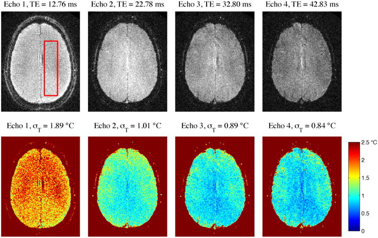
Baseline magnitude of each echo of ME_HighRes (top row) with temperature uncertainties calculated from each echo individually (bottom row). σ_T indicates average temperature uncertainty within an ROI, delineated by the red box.

Off-Resonance Correction

To demonstrate the effect of multi-frequency reconstruction, an additional scan was performed in a region of the brain with greater off-resonance variation, and without higher-order shim correction. Fig 2 shows the baseline magnitude for ME_Fast for that scan, before and after multi-frequency reconstruction. The estimated off-resonance is included. The sum-of-squares algorithm was used to combine magnitude images across echoes. In the acquired images, off-resonance spiral artifacts corrupt the edges of the brain and clarity of features within the brain. The multi-frequency reconstruction restores sharpness of boundaries and structures in the image, some of which are highlighted with arrows in the figure.

Figure 2.

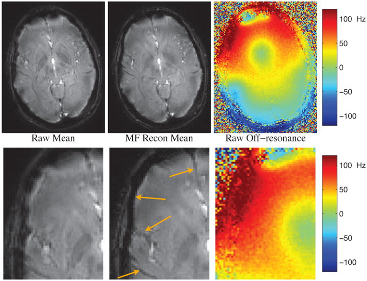
Comparison of sum-of-squares baseline magnitude before (left) and after (center) multi-frequency reconstruction every 10 Hz, with off-resonance shown pre-correction (right). Bottom row is zoomed to better show regions with significant improvement. Arrows point to features that have been more sharply resolved after multi-frequency recon.

Flip Angle Optimization

To determine optimal flip angles in vivo, each of the sequences was run across a range of flip angles in a single scan session. The relative SNR vs flip angle for each sequence is shown in Fig 3. Relative SNR for ME_2DFT peaked at the lowest flip angle (9°) and decreased more rapidly than other sequences for larger flip angles. ME_Precise, with the longest TR, reached its peak at the highest flip angle (14°). The other three sequences were similar, with ME_Fast reaching its peak at 12° and ME_HighRes and 2DFT each peaking at 11°. The peak signal flip angles were used for in vivo temperature uncertainty measurement.

Figure 3.

Relative SNR vs Flip Angle for each sequence. Sampled points are marked with an asterisk, intermediate positions are spline interpolated. ME_HighRes is shown with a dashed line to avoid obscuring ME_Fast.

In Vivo Temperature Uncertainty

Baseline magnitude images for each sequence are shown in the top row of Fig 4, for one of the volunteer in vivo scans. Multiple-echo sequences are shown using sum-of-squares combination of the individual echo magnitudes. Geometric fidelity appears similar across the sequences, though subcutaneous fat appears shifted in the low bandwidth 2DFT sequence. Temperature uncertainty for each sequence is displayed in the bottom row of Fig 4, with average uncertainties included in the figure titles. Table 2 compiles the average in vivo results across subjects and the relative efficiencies of the sequences. ME2DFT has 106% of the efficiency of 2DFT, while the multi-echo spiral sequences improve efficiency by factors of 2.4-3.2.

Figure 4.

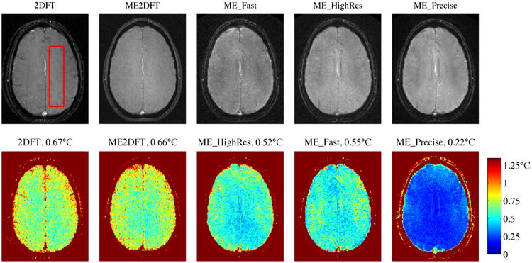
Baseline (4 frame average) magnitude (top row) and temperature uncertainty (bottom row) for each sequence, (volunteer 3). Red box indicates ROI used for spatial average of temperature uncertainty. Sum-of-squares used to combine multiple echo baselines. Uncertainties calculated with tSNR-optimal echo combination. Average uncertainties indicated in titles.

Table 2. Average uncertainty and sequence efficiency for each of the five sequences.

	2DFT	ME2DFT	ME_Fast	ME_HighRes	ME_Precise
Resolution (mm)	1.09 × 2.19	1.09 × 2.19	1.49 × 1.49	1.09 × 1.09	1.49 × 1.49
Sequence Time	3.61 sec	3.46 sec	1.07 sec	3.63 sec	3.53 sec
Linear Frequency Fit Uncertainty		1.58°C	1.32°C	1.30°C	0.50°C
tSNR-Optimal Uncertainty	0.67°C	0.64°C	0.54°C	0.50°C	0.23°C
Normalized tSNR Efficiency	100%	106%	244%	270%	316%

The high precision sequence (ME_Precise) had the greatest overall efficiency of the sequences tested in this work, improving uncertainty (relative to 2DFT) by 2.9× with 7% smaller voxels and 2% faster scan time. The ME_HighRes sequence achieved 2× better resolution than 2DFT, with 33% better uncertainty and the same scan time. The ME_Fast sequence achieved 3.4× faster imaging, with 7% better resolution than 2DFT and 23% better temperature uncertainty.

Table 2 also includes the average temperature uncertainties that are obtained using linear-fitting reconstruction. Uncertainties with the linear-fit were significantly worse than the tSNR-optimal echo combination reconstruction, ranging from 2.2-2.6× higher for the multi-echo sequences. Table 3 compiles the echo-combination temperature uncertainties for each sequence for each volunteer, to show how sequence performance varies across subjects. Paired t-tests showed that the uncertainties for each pair of sequences were significantly different (p<0.05), except for the pairs {2DFT, ME2DFT} and {ME_Fast, ME_HighRes}.

Table 3. Temperature uncertainty for each sequence, using tSNR-optimal echo combination, across volunteers.

	2DFT	ME2DFT	ME_Fast	ME_HighRes	ME_Precise
Volunteer 1	0.68°C	0.66°C	0.59°C	0.53°C	0.27°C
Volunteer 2	0.64°C	0.60°C	0.47°C	0.45°C	0.20°C
Volunteer 3	0.67°C	0.66°C	0.55°C	0.52°C	0.22°C
Average	0.67°C	0.64°C	0.54°C	0.50°C	0.23°C

Phantom Heating Results

The heating time curves measured during each phantom sonication are shown in Fig 5. Circles indicate the sampled time points, with lines connecting each sampled point. No lines connect the time points immediately prior to and immediately following sonication, as the timing difference between those points is uncertain. Temperatures during cooling appear very similar for all sequences, while the peak measured temperatures and observed temperatures during heating vary slightly across sequences. The peak measured temperatures are listed in Table 4, along with the temperature uncertainty measured in an unheated area of the phantom for each sequence. Full-width half-maximum (FWHM) of the heating profile was approximately 3 mm, as measured in the ME_HighRes data. Assuming a 3 mm FWHM Gaussian profile, spatial averages over the voxel dimensions for each sequence were calculated (“Under-prediction Due to Resolution”) and used to estimate actual peak heating (“Corrected Temperature”), with values listed in Table 4. As an example to illustrate this metric, an actual 10°C peak temperature rise would yield an expected 8.6°C measurement from the voxel size used by 2DFT. While measured peak temperatures varied by 2.34°C across sequences, correction for resolution effects reduced the variation to 1.46°C. Exclusion of the ME2DFT peak temperature, whose peak appears to be a noisy outlier in the temperature curve shown in Fig 5, reduces the corrected peak temperature variation to 1.08°C across the four remaining sequences. Focal spot temperature images, interpolated to an estimated 12 sec after sonication onset, are displayed in Fig 6. The spiral voxels have isotropic in-plane resolution, and show circular focal spot shapes. The 2DFT sequences have rectangular voxels, with the phase encode dimension appearing left-right in the figure. This anisotropic resolution results in asymmetric focal spots. In all cases, the displayed resolution is 0.55 mm isotropic, regardless of the sequence's acquired resolution. (The apparent offset of ME_HighRes relative to the other spiral sequences is an artifact of the upsampling algorithm used.) Higher peak temperature is visible in the center of focus in the high-resolution sequence.

Figure 5.

Heating curves for each sequence. Circles indicated sampled time points.

Table 4.

Maximum temperature measured during phantom heating for each sequence, with temperature uncertainty. Simulated under-prediction is fraction of peak temperature expected assuming 3 mm FWHM Gaussian temperature distribution, and is used to correct measured temperature for last row.

	2DFT	ME2DFT	ME_Fast	ME_HighRes	ME_Precise
Maximum Temperature	14.26°C	15.52°C	15.51°C	16.6˚C	14.85°C
Temperature Uncertainty	0.30°C	0.35°C	0.20°C	0.20°C	0.071°C
Under-prediction Due to Resolution	0.86	0.86	0.89	0.94	0.89
Corrected Temperature	16.6°C	18.0°C	17.4°C	17.7°C	16.7°C

Figure 6.

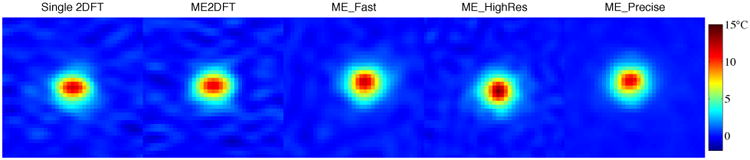
Heated spot, interpolated to 12 sec after heating onset, for each sequence. FOV zoomed to 16 mm to show detail. Each image upsampled to 0.55 mm resolution. Apparent offset of ME_HighRes is due to upsampling

Discussion

Multiple-echo spiral echo sequences were demonstrated to significantly improve MR temperature monitoring, as compared to standard 2DFT thermometry. Off-resonance spiral artifacts were minimized by using short readout durations (21) and with post-gridding multi-frequency reconstruction. Temperature reconstruction with tSNR-optimal echo combination demonstrated reduced multi-echo temperature uncertainty. The use of spiral trajectories enables acquisitions with fewer TRs, which allows for greater temperature accuracy through lengthened TEs and TRs. These allowed for improved resolution, speed, or precision, with demonstrated efficiency improvements of 2.4-3.2× as compared to 2DFT thermometry.

Off-Resonance Correction

The spiral duration and multi-frequency reconstruction approach used in this work was sufficient for avoiding off-resonance artifacts in the in vivo and phantom experiments, with the pre- and post- correction images in Fig 2 showing the effect of proper reconstruction. Off-resonance during spiral readouts does not generate geometric shift, which will help to ensure that the location of measured heating is accurately interpreted. When designing sequences for specific applications, the amount and variability of off-resonance in the object being imaged can lead to different optimal design trade-offs between efficiency (longer spirals) and robustness to off-resonance. Updating off-resonance estimates on a per-frame basis to inform multi-frequency reconstruction, or using more finely sampled frequencies in reconstruction, would reduce the maximal off-resonance, allowing for increased spiral durations and efficiency at the cost of increased reconstruction complexity.

Multiple-echo Uncertainty Performance In Vivo

Multi-echo 2DFT was demonstrated with efficiency matching that of 2DFT thermometry. The 2DFT sequence used 11.36 kHz sampling bandwidth while ME2DFT used 9 readouts each with 125 kHz sampling. The 18% reduction in sampling time for ME2DFT predicts a 9.5% worsening of uncertainty, which was not observed in vivo. The 11× increase in readout bandwidth significantly reduces off-resonance shift artifacts and could more accurately measure the location of heating, while still employing conventional readouts and image reconstruction. Multi-echo 2DFT additionally provides real-time estimates of T2*, off-resonance, and T1-weighted proton density (by estimating magnitude at TE=0).

Multi-echo spiral thermometry allows for improved temperature monitoring efficiency, which can be used to improve various design objectives. In this work, multi-echo spirals were successfully used to improve design objectives without worsening other performance metrics. The sequences were able to double resolution, improve precision by 2.9×, or speed up the sequence by 3.4×, with efficiency improvements of 2.4× or greater as compared to 2DFT. These efficiency improvements can be reallocated in different ways for any specific application, depending on the monitoring needs of that application, with the design points demonstrated in this work showing a coarse estimate of the improved design frontier. While multi-slice monitoring was not shown in this work, the ME_Fast sequence can also be used for 3-slice interleaved monitoring with 3.24 second update rate and improved uncertainty, (resulting from increased T1 recovery using a longer TR,) so volumetric coverage can be traded off with speed, precision, and resolution as well. Relative performance comparisons between 2DFT and the multi-echo spirals assume a specific tissue type, as the benefit of increased TE and TR depend on MRI tissue parameters. Translation of multi-echo spiral imaging to other tissue types should also provide improved performance over single-echo 2DFT, but the relative improvement may be different than was demonstrated in brain. Within the brain, restricting imaging to only gray matter or only white matter would similarly effect the relative performance measured between each sequence, and would lead to different optimal imaging sequence parameters.

The significant performance improvements of the multi-echo spiral sequences, and adequate performance of multi-echo 2DFT, depend on proper temperature reconstruction. Direct comparison of reconstruction techniques showed that the tSNR-optimal echo combination performed more than twice as well as linear fitting of phase vs TE. (Selection of different TEs will result in differences in the relative performance.) One caveat to these findings is that the echo combination approach assumes that the phase at TE=0 does not change over time, which may not be the case (26). If future work determines that there is an explicit relationship between phase at TE=0 and heating, then a new model can be used to estimate temperature for each echo, and maintain the performance advantage of echo combination reconstruction.

Phantom Heating Thermometry

During repeated heatings of a phantom, monitoring with each sequence yielded similar temperature curves, with some differences during heating and very similar cooling curves. The ME_Fast sequence detected temperature changes more rapidly after sonication onset and offset, as expected from the improved temporal resolution. Some differences in measured heating are expected due to imperfect repeatability of the heating experiment. During sonication, the heating curves appeared similar but with different scaling, with the 2DFT and ME2DFT sequences yielding lower temperatures and the ME_HighRes sequence yielding a higher temperature. Much of this discrepancy can be explained by spatial resolution effects, and correction for these effects yielded strong agreement between each of the heating tests. While transcranial patient treatments have heating profiles with approximately 6 mm FWHM in the axial plane, (resulting in lesions that are 3-4 mm in diameter), the phantom experiment had significantly narrower heating with approximately 3 mm FWHM. This results in an expected 14% underestimation of phantom peak heating by the 2DFT spatial resolution, while it would underestimate a 6 mm FWHM profile by only 4%. In an in vivo application with a broader focal spot, all of the sequences are expected to measure peak temperature accurately. It is possible that some difference in measured temperature are due to errors in the assumed coefficient between temperature changes and phase changes. While reconstruction for all sequences assumed α = -0.01 ppm/°C, the spiral sequences utilized longer TE than is conventionally used, and previous work has observed TE-dependence in the temperature coefficient (26). However, the strong agreement between the ME_Fast and ME_Precise curves (which utilized different echo times) suggests that this factor was not significant. While external temperature measurement was not achievable with this tested experimental setup, the general agreement between the heatings across sequences suggests that each of the sequences are measuring focal heating with similar accuracy. Future monitoring with concurrent external measurement of the focal temperature would help to validate the accuracy of the proposed multi-echo sequences and also provide estimates of α as a function of echo time.

Impact of Low SNR

An issue that multiple-echo thermometry is susceptible to that single-echo thermometry generally is not is that of low image SNR. Temperature measurements depend on accurate measurement of phase, with phase SNR and magnitude SNR being proportional for sufficiently high magnitude SNR. For low magnitude SNR, phase measurements deteriorate rapidly, and can prevent meaningful temperature monitoring. When designing sequences for a specific application and hardware setup, TEs must be selected to maximize efficiency (longer TE) while ensuring sufficient SNR, to obtain optimal thermometry performance. In this work, maximum TE of the ME_HighRes and ME_Fast sequences were limited to ∼40 ms because of low SNR at longer echo times, while ME_Precise used lower sampling bandwidth for improved SNR and could utilize longer TEs of ∼60 ms. Improvements in imaging SNR through hardware changes (such as increased field strength or improved coil sensitivity) can therefore yield super-linear temperature SNR improvements when using multi-echo spiral thermometry, as the increased SNR may enable longer echo times for more efficient sequences.

Conclusions

In this work, multiple-echo spiral thermometry has been proposed and validated as a means for improved MRI temperature monitoring in brain. Sequence efficiency was improved by 2.4× - 3.2× when compared to 2DFT monitoring. These improvements could allow for better treatment monitoring if applied to clinical thermometry, by providing faster, more precise, or higher resolution measurements. Multiple-echo 2DFT monitoring was also demonstrated, as a high bandwidth alternative to conventional 2DFT monitoring with similar temperature uncertainty. The higher bandwidth reduces shift artifacts from off-resonance by a factor of 5.5, (11 in each direction but with opposing directions for alternate echoes,) potentially improving geometric registration between measured heating and underlying anatomical images.

References

- 1.Elias WJ, Huss D, Voss T, et al. A pilot study of focused ultrasound thalamotomy for essential tremor. N Engl J Med. 2013;369:640–648. doi: 10.1056/NEJMoa1300962. [DOI] [PubMed] [Google Scholar]
- 2.Martin E, Jeanmonod D, Morel A, Zadicario E, Werner B. High-intensity focused ultrasound for noninvasive functional neurosurgery. Ann Neurol. 2009;66:858–861. doi: 10.1002/ana.21801. [DOI] [PubMed] [Google Scholar]
- 3.Jeanmonod D, Werner B, Morel A. Transcranial magnetic resonance imaging–guided focused ultrasound: noninvasive central lateral thalamotomy for chronic neuropathic pain. Neurosurg Focus. 2012;32:1–11. doi: 10.3171/2011.10.FOCUS11248. [DOI] [PubMed] [Google Scholar]
- 4.McDannold N, Clement GT, Black P, Joelesz F, Hynynen K, Smyth M. Transcranial MRI-guided focused ultrasound surgery of brain tumors: Initial finding in three patients. Neurosurgery. 2010;66:323–332. doi: 10.1227/01.NEU.0000360379.95800.2F. [DOI] [PMC free article] [PubMed] [Google Scholar]
- 5.Ishihara Y, Calderon A, Watanabe H, Okamoto K, Suzuki Y, Kuroda K. A precise and fast temperature mapping using water proton chemical shift. Magn Reson Med. 1995;34:814–823. doi: 10.1002/mrm.1910340606. [DOI] [PubMed] [Google Scholar]
- 6.Rieke V, Butts Pauly K. MR thermometry. J Magn Reson Imaging. 2008;27:376–390. doi: 10.1002/jmri.21265. [DOI] [PMC free article] [PubMed] [Google Scholar]
- 7.Todd N, Vyas U, de Bever J, Payne A, Parker DL. The effects of spatial sampling choices on MR temperature measurements. Magn Reson Med. 2011;65:515–521. doi: 10.1002/mrm.22636. [DOI] [PMC free article] [PubMed] [Google Scholar]
- 8.Quesson B, de Zwart J, Moonen CT. Magnetic resonance temperature imaging for guidance of thermotherapy. J Magn Reson Imaging. 2000;12:525–533. doi: 10.1002/1522-2586(200010)12:4<525::aid-jmri3>3.0.co;2-v. [DOI] [PubMed] [Google Scholar]
- 9.De Zwart JA, Vimeux C, Delalande C, Canioni P, Moonen CTW. Fast lipid-suppressed MR temperature mapping with echo-shifted gradient-echo imaging and spectral-spatial excitation. Magn Reson Med. 1999;42:53–9. doi: 10.1002/(sici)1522-2594(199907)42:1<53::aid-mrm9>3.0.co;2-s. [DOI] [PubMed] [Google Scholar]
- 10.Köhler MO, Mougenot C, Quesson B, Enholm J, Le Bail B, Laurent C, Moonen CTW, Ehnholm GJ. Volumetric HIFU ablation under 3D guidance of rapid MRI thermometry. Med Phys. 2009;36:3521–3535. doi: 10.1118/1.3152112. [DOI] [PubMed] [Google Scholar]
- 11.Roujol S, Ries M, Quesson B, Moonen C, Denis de Senneville B. Real-time MR-thermometry and dosimetry for interventional guidance on abdominal organs. Magn Reson Med. 2010;63:1080–1087. doi: 10.1002/mrm.22309. [DOI] [PubMed] [Google Scholar]
- 12.Quesson B, Laurent C, Maclair G, de Senneville BD, Mougenot C, Ries M, Carteret T, Rullier A, Moonen CTW. Real-time volumetric MRI thermometry of focused ultrasound ablation in vivo: a feasibility study in pig liver and kidney. NMR Biomed. 2011;24:145–153. doi: 10.1002/nbm.1563. [DOI] [PubMed] [Google Scholar]
- 13.Schmidt R, Frydman L. Alleviating artifacts in 1H MRI thermometry by single scan spatiotemporal encoding. Magn Reson Mater Physics, Biol Med. 2013;26:477–490. doi: 10.1007/s10334-013-0372-9. [DOI] [PubMed] [Google Scholar]
- 14.Pruessmann KP, Weiger M, Scheidegger MB, Boesiger P. SENSE: Sensitivity encoding for fast MRI. Magn Reson Med. 1999;42:952–962. [PubMed] [Google Scholar]
- 15.Mulkern RV, Panych LP, Hynynen K, Jolesz FA, McDannold NJ. Tissue temperature monitoring with multiple gradient-echo imaging sequences. J Magn Reson Imaging. 1998;8:493–502. doi: 10.1002/jmri.1880080234. [DOI] [PubMed] [Google Scholar]
- 16.Todd N, Diakite M, Payne A, Parker DL. In vivo evaluation of multi-echo hybrid PRF/T1 approach for temperature monitoring during breast MR-guided focused ultrasound surgery treatments. Magn Reson Med. 2014;72:793–799. doi: 10.1002/mrm.24976. [DOI] [PMC free article] [PubMed] [Google Scholar]
- 17.Li C, Pan X, Ying K, Zhang Q, An J, Weng D, Qin W, Li K. An internal reference model-based PRF temperature mapping method with Cramer-Rao lower bound noise performance analysis. Magn Reson Med. 2009;62:1251–1260. doi: 10.1002/mrm.22121. [DOI] [PubMed] [Google Scholar]
- 18.Rieke V, Butts Pauly K. Echo combination to reduce proton resonance frequency (PRF) thermometry errors from fat. J Magn Reson Imaging. 2008;27:673–677. doi: 10.1002/jmri.21238. [DOI] [PMC free article] [PubMed] [Google Scholar]
- 19.Madore B, Panych LP, Mei CS, Yuan J, Chu R. Multipathway sequences for MR thermometry. Magn Reson Med. 2011;66:658–668. doi: 10.1002/mrm.22844. [DOI] [PMC free article] [PubMed] [Google Scholar]
- 20.Yudilevich E, Stark H. Spiral sampling in magnetic resonance imaging-the effect of inhomogeneities. IEEE Trans Med Imaging. 1987;6:337–345. doi: 10.1109/TMI.1987.4307852. [DOI] [PubMed] [Google Scholar]
- 21.Maeda A, Sano K, Yokoyama T. Reconstruction by weighted correlation for MRI with time-varying gradients. IEEE Trans Med Imaging. 1988;7:26–31. doi: 10.1109/42.3926. [DOI] [PubMed] [Google Scholar]
- 22.Noll DC. Methodologic considerations for spiral k-space functional MRI. Int J Imaging Syst Technol. 1995;6:175–183. [Google Scholar]
- 23.Irarrazabal P, Meyer CH, Nishimura DG, Macovski A. Inhomogeneity correction using an estimated linear field map. Magn Reson Med. 1996;35:278–282. doi: 10.1002/mrm.1910350221. [DOI] [PubMed] [Google Scholar]
- 24.Noll DC, Meyer CH, Member S, Pauly JM, Nishimura DG, Macovski A. A homogeneity correction method for magnetic resonance imaging with time-varying gradients. IEEE Trans Med Imaging. 1991;10:629–637. doi: 10.1109/42.108599. [DOI] [PubMed] [Google Scholar]
- 25.Man L, Pauly J, Macovski A. Improved automatic off-resonance correction without a field map in spiral imaging. Magn Reson Med. 1997;37:906–913. doi: 10.1002/mrm.1910370616. [DOI] [PubMed] [Google Scholar]
- 26.Peters RD, Henkelman RM. Proton-resonance frequency shift MR thermometry is affected by changes in the electrical conductivity of tissue. Magn Reson Med. 2000;43:62–71. doi: 10.1002/(sici)1522-2594(200001)43:1<62::aid-mrm8>3.0.co;2-1. [DOI] [PubMed] [Google Scholar]