Interactive analysis and assessment of single-cell copy-number variations

Abstract

We present an open-source web platform, Ginkgo (http://qb.cshl.edu/ginkgo), for the analysis and assessment of single-cell copy-number variations (CNVs). Ginkgo automatically constructs copy-number profiles of cells from mapped reads and constructs phylogenetic trees of related cells. We validate Ginkgo by reproducing the results of five major studies and examine the characteristics of three commonly used single-cell amplification techniques to conclude degenerate oligonucleotide-primed PCR to be the most consistent for CNV analysis.

Single-cell sequencing¹ has become an important tool for probing cancer², neurobiology³, developmental biology^4–6, and other complex systems. Studying genomic variation at the single-cell level allows investigators to unravel the genetic heterogeneity within a sample and enables the phylogenetic reconstruction of subpopulations beyond what is possible with standard bulk sequencing, which averages signals over millions of cells. To date, thousands of individual human cells have been profiled to map the subclonal populations within cancerous tumors⁷ and circulating tumor cells⁸, to discover mosaic copy-number variations in neurons³, and to identify recombination events within gametes^{5, 9}, among many other applications. One key application of single-cell sequencing is to identify large-scale (>10kb) copy-number variations (CNVs)^{3, 7, 10}. For example, in cancer, CNVs form a “genetic fingerprint” from which one can infer the phylogenetic history of a tumor¹¹ and trace progression of metastatic events⁷.

Given the insights made possible by single-cell sequencing, many researchers are now interested in applying the technology to study diverse biological systems and species. However, the downstream analysis is complex. Although many approaches and computational tools exist for CNV analysis of bulk samples¹² there are currently no fully automated and open-source tools that address the unique challenges of single-cell sequencing data: (1) extremely low depth of sequencing coverage (< 1X) makes for noisy profiles and makes split-read, paired-end, or SNP density approaches ineffective; (2) whole-genome amplification (WGA) biases markedly distort read counts, including failure to amplify entire segments¹³; (3) badly assembled regions of the genome (e.g. centromeres) lead to the artificial inflation of read counts (“bad bins”)¹³; (4) calling copy number at single-cell, integer levels requires development of new algorithms; and (5) exploring population structure is not needed, and often not possible, in bulk sequencing. In addition, several unique sources of cell-specific errors are introduced during the experimental procedures, including GC content and other sequencing biases. While ad hoc methods have been developed for individual studies, there is currently no easy-to-use, open-source software available that executes this pipeline automatically and correctly.

Here we present our new open-source web analytics platform, Ginkgo, for the automated and interactive analysis of single-cell copy-number variations. Ginkgo enables researchers to upload samples, select processing parameters, and after processing, explore the population structure and cell-specific variants revealed within a visual analytics framework in their web browser.

Ginkgo guides users through every aspect of the analysis in a user-friendly interface, from binning reads into regions across the genome, to quality assessment, GC bias correction, segmentation, copy-number calling, visualization and exploration of results (Fig. 1). This pipeline builds on our previous single-cell sequencing work¹³, and includes several novel features not previously described to advance the state of the art, including: (1) a new algorithm for determining absolute copy-number state from the segmented raw read depth, (2) a new method for controlling quality issues in the reference assembly (see “bad bins” in Online Methods); (3) an option to integrate ploidy information from fluorescence-activated cell sorting (FACS) to accurately call copy number; and (4) a suite of interactive visual analytics tools to allow users to easily share results with collaborators and clinicians. Ginkgo provides functionality for five different species (human, chimp, mouse, rat, and fly) and includes a wide array of tunable parameters for individual users’ needs (Online Methods).

Figure 1.

The Ginkgo flowchart for performing single-cell copy-number analysis. Usage and parameters are described in the online methods and on the website.

Once an analysis completes, Ginkgo displays an overview of the data in a sortable data table, an interactive phylogenetic tree¹⁴ of all cells used in the analysis, and a set of heat maps detailing the CNVs that drove the clustering results. Clicking on a cell in the interactive phylogenetic tree or data table allows the user to view an interactive plot of the genome-wide copy-number profile of that cell, search for genes of interest, and link out to a custom track of amplifications and deletions in the UCSC genome browser. Ginkgo also outputs several quality assessment graphs for each cell: a plot of read distribution across the genome, a histogram of read count frequency per bin, and a Lorenz curve to assess coverage uniformity¹⁵. Subsets of interesting cells can also be selected by the user to directly compare copy-number profiles, Lorenz curves, GC bias, and coverage dispersion.

To validate Ginkgo, we set out to reproduce the major findings of five single-cell studies that used either multiple annealing and looping-based amplification (MALBAC) or DOP-PCR amplification (Supplementary Note 1). These datasets address vastly different scientific questions, were collected from a variety of tissue types, and make use of different experimental and computational approaches at different institutions. Using Ginkgo, we replicated the vast majority of published CNVs for each cell in each of the datasets with the exception of one cell in Hou et al., which we believe was due to mislabeling in the National Center for Biotechnology Information (NCBI) short-read archive (SRA). Moreover, the Navin et al. and Ni et al. datasets used the identified CNVs to generate phylogenetic trees across all samples. Ginkgo is able to reproduce the distinct clonal subpopulations in the two Navin et al. datasets (Supplementary Fig. 1) and the patient clustering results from Ni et al. (Supplementary Fig. 3). Using simulated copy-number profiles we confirm that Ginkgo reliably identifies copy-number changes (98.8% accuracy, 98.7% true positive rate, 1.2% false positive rate) and perfectly reproduces the population structure through clustering of the individual samples (Online Methods).

While Ginkgo corrects for many of the biases present in single-cell data, higher quality data inevitably leads to higher quality results. In order to explore the effects of WGA on data quality, we set out to compare the biases and differences in coverage uniformity between the three most widely published WGA techniques: multiple displacement amplification (MDA), MALBAC, and DOP-PCR using 9 distinct datasets, 3 for each method.

Raw sequencing reads from each of nine datasets were downloaded from NCBI (Online Methods). Reads were mapped to the human genome and downsampled to match the lowest coverage sample. Finally, aligned reads were binned into 500kb variable-length intervals across the genome such that the intervals average 500kb in length but contain the same number of uniquely mappable positions (see Online Methods). We use these binned read counts to measure two key data quality metrics: GC bias and coverage dispersion. Importantly, raw bin counts provide a robust view of the data quality impartial to the different approaches to segmentation, copy-number calling, or clustering.

GC content bias refers to preferential amplification and sequencing because of the percentage of G+C nucleotides in a given region of the genome¹⁶. This introduces cell-specific and library-specific correlations between GC content and bin counts. In particular, when GC content in a genomic region falls outside a certain range (typically <0.4 or >0.6), read counts rapidly decrease (Online Methods). We find that MDA has very high GC bias compared to MALBAC and DOP-PCR (Fig. 2a). Only 45.9% of MDA bin counts fall within the expected coverage range compared to 94.0% of MALBAC bin counts and 99.6% of DOP-PCR bin counts. It is important to note that, regardless of WGA approach, each cell has unique GC biases that must be individually corrected.

Figure 2.

(a) Lowess fit of GC content with respect to log normalized bin counts for all samples in each of the 9 datasets analyzed: 3 for MDA (top left – green), 3 for MALBAC (center left – orange), and 3 for DOP-PCR (bottom left – blue). Each colored line within a plot corresponds to the lowess fit of a single sample. The dashed lines show a two fold increase or decrease in average observed coverage. Note that the three MDA datasets (top left) have a different y-axis scale due to the large GC biases present. (b) The median absolute deviation (MAD) of neighboring bins: A single pair-wise MAD value is generated for each sample in a given dataset and represented by a box and whisker plot. The bold center line represents the mean, the box boundaries represent the quartiles, and the whiskers represent the remaining data points. The high biases present in the MDA datasets make comparing DOP-PCR and MABLAC samples difficult. Figure 3 of the Online Methods shows this comparison more clearly.

As a further measure of data quality, we calculated the median absolute deviation (MAD) of all pair-wise differences in read counts between neighboring bins for each sample, after normalizing the cells by dividing the count in each bin by the mean read count across bins. MAD is resilient to outliers caused by copy-number breakpoints, as transitions from one copy-number state to another are relatively infrequent. Instead, pair-wise MAD reflects the bin count dispersion due to technical noise. For each of the nine datasets, the MAD was calculated for each cell and displayed in a box-and-whisker plot (Fig. 2b). As expected from previous comparisons of MDA to other WGA techniques^{15, 17}, MDA data displays high levels of coverage dispersion on average, with a mean MAD 2 to 4 times that of the DOP-PCR datasets. In addition, the MALBAC and MDA datasets show large differences in data quality between studies while the DOP-PCR datasets show consistent flat MAD across all three studies (Supplementary Fig. 3).

We find that DOP-PCR outperforms both MALBAC and MDA in terms of data quality. As previously reported^{15, 17–20}, MDA displays poor coverage uniformity and low signal-to-noise ratios. Coupled with overwhelming GC biases, MDA is unreliable for accurately determining CNVs compared to the other two techniques. Furthermore, while both DOP-PCR and MALBAC data can be used to generate CNV profiles and identify large variants, DOP-PCR data has substantially lower coverage dispersion and smaller GC biases when compared to MALBAC data. Given the same level of coverage, our results indicate that data prepared using DOP-PCR can reliably call CNVs at higher resolution with better signal-to-noise ratios, and is more reliable for accurate copy-number calls.

Online Methods

1. Code availability

The source code for Ginkgo is available open source at https://github.com/robertaboukhalil/ginkgo and is preinstalled at http://qb.cshl.edu/ginkgo. It provides a large number of user specified parameters to control how the analysis is performed and how the results are interpreted (Supplementary Table 1). Several of these must be set according to the experimental design of the study (genome, bin size, sex chromosome masking, FACS copy number estimation), while others allow the researcher to explore the analysis using different metrics depending on the goals of the study. See the sections below for a more complete description.

1.a. Binning method

Copy number analysis begins with binning uniquely mapping reads into fixed-length or variable-length intervals across the genome. This aggregates read depth information into larger regions that are more robust to variable amplification and other biases. As discussed in the main text, fixed-length bins are generally discouraged as they lead to read drop out in regions that span highly repetitive regions, centromeres, and other complex genomic regions.

To generate boundaries for variable-length bins, we use the method outlined by Navin et al. (2010), where we sample 101bp stretches of the reference assembly at every position along the genome. These simulated reads are mapped back to the genome using Bowtie and only uniquely mapping reads are analyzed. For a given bin size, we assign reads into bins such that each bin has the same number of uniquely-mappable reads. Consequently, intervals with higher repeat content and low mappability will be larger than intervals with highly mappable sequences, although they will both have the same number of uniquely mappable positions.

Using variable-length bins with sufficient depth of coverage and consistent ploidy, sequence reads are expected to map evenly across the entire genome with uniform variance. Users are provided with a variety of bin sizes from which to choose, depending on the overall coverage available; if the mean coverage per bin is too low, we encourage users to use larger bins.

1.b. Masking bad bins

As described in the main text, there are a number of regions, specifically around the centromeres of certain chromosomes, where there is an accumulation of very high read depth compared to the expected depth. These regions consistently display high read depth in both bulk and single-cell sequencing data. Using data from 54 normal individual diploid cells from multiple individuals (not presented here), these bins (designated as “bad bins”) were determined in the human reference genome (hg19) as follows. The bin counts were divided by the mean bin counts for each cell to normalize for differences between cells in total read count. For each chromosome, the mean of the bins over all cells is subtracted from each individual cell’s normalized bin count to normalize for differences between chromosomes. The mean and standard deviation of the autosomes is then used to compute an outlier threshold corresponding to a p-value of 1/N, where N is the number of bins used. In practice, less than 1% of bins are identified as extreme outliers and masked for further processing.

1.c. GC bias correction

Once reads are placed into bins, Ginkgo normalizes each sample and corrects for GC biases prior to segmentation. The normalization process begins by dividing the count in each bin by the mean read count across all bins. This centers the bin counts of all samples at 1.0. To identify and correct GC biases, Ginkgo computes a locally-weighted linear regression using the R function lowess (smoother span = .5, iterations = 3, delta=0.1*range(x)) to model the relationship between GC content and log-normalized bin counts. This lowess fit is then used to scale each bin such that the expected average log-normalized bin count across all GC values is zero. After the lowess fit, we monitor the bias of each cell by calculating the proportion of bins that fall outside an expected coverage of zero by +/− 1, log base 2.

1.d. Segmentation (CBS)

Following GC bias correction, bin counts are segmented to reduce fluctuations in noise across chromosomes and identify longer regions of equal copy number. To this end, Ginkgo makes use of Circular Binary Segmentation (CBS), which segments the genome by recursively splitting the chromosomes into segments based on a maximum t-statistic until a reference distribution estimated by permutation is reached. Once the CBS segmentation is complete, the breakpoints (segment boundaries) across all bins are determined, and the counts for all bins within each segment are reset to be the median bin count value within that segment.

The key step during segmentation is selecting the right reference sample for comparison. Using a diploid sample to normalize bin counts can eliminate additional biases uncorrected by GC normalization. Although Ginkgo supports uploading data from such a cell, this is not always available so Ginkgo provides alternatives for segmenting samples: (1) Independent segmentation, where samples are segmented independently by their own normalized bin count profiles; and (2) Sample with lowest IOD, where Ginkgo selects the sample with the lowest index of dispersion (IOD - the ratio between the read coverage variance and the mean) and uses that sample as a reference for all other samples. The sample with the lowest index of dispersion will likely be among the most evenly balanced ploidy and highest quality of all submitted cells.

1.e. Determining copy-number state

Since we are analyzing single-cell data, we expect every genomic locus to have an integer copy number (CN) value. Furthermore, the quantized nature of single-cell data means that the same number of reads per bin should separate every sequential CN state, e.g., ~50 reads for CN 1, ~100 reads for CN 2, ~150 reads for CN 3, etc. While biological and technical noise prevent read counts from segregating perfectly into distinct CN states, read counts should still be centered around integer CN states.

The most direct approach for determining the CN state of each cell is available for users that have a priori knowledge of the ploidy of each sample. For example, cells that are DAPI-stained prior to cell sorting can be gated based on their fluorescence activity, and ploidy can be determined by comparing its fluorescence activity to that of a reference cell with a known CN state. With these data, Ginkgo determines the copy number state of each sample by scaling the segmented bin counts such that the mean bin count is equal to the ploidy of the sample. Finally bin counts are rounded to integer copy number values. Advances in fluorescence activated cell sorting (FACS) will make this copy number prediction even more accurate in time, although cells that are incorrectly sorted and placed into wells with more than one cell will show much higher fluorescence activity and will have an incorrectly inferred copy number state.

Since FACS data is not always available for analysis and has potential for error, Ginkgo provides an alternative to determine the copy number of each sample. As discussed earlier, before determining the CN state of a cell, the cell is binned, normalized, and segmented. This copy number profile has a mean of one and is referred to as the raw copy number profile (RCNP). If the true genome-wide copy number of a sample were equal to X, the scaled copy number profile (SCNP) would then be the product of RCNP and X, and the final integer copy number profile (FCNP) would be the rounded value of the SCNP so all segments contain an integer value.

With these relationships, Ginkgo infers the genome-wide copy number X using numerical optimization. For a given cell, Ginkgo first determines the SCNP and FCNP for all possible values of X in the set [1.50, 1.55, 1.60, …, 5.90, 5.95, 6.00]. Ginkgo then computes the sum of square (SoS) error between the SCNP and the RCNP for each value of X and selects the value of X with the smallest SoS error. Once the multiplier is identified and applied, the scaled bins are rounded to generate the final integer copy number profile for each sample. Intuitively, this is equivalent to finding the copy number multiplier that causes the normalized segmented bin counts to best align with integer copy number values.

1.f. Clustering

Before visualization, the final step is to look outside the scope of individual cells and determine the overall population structure. Ginkgo first determines the distance (dissimilarity structure) between all cells. We provide six choices of distance metrics: Euclidean, maximum, Manhattan, Canberra, binary, and Minkowski. After computing the dissimilarity matrix, Ginkgo then computes a dendrogram through neighbor joining or by hierarchically clustering samples using one of four different agglomeration methods: single linkage, complete linkage, average linkage, and ward linkage. In addition, Ginkgo generates a phylogenetic tree by first computing the Pearson correlation between all samples and using these dissimilarity values to cluster the samples.

1.g. Masking sex chromosomes

Careful consideration of gender must be given when analyzing patients from mixed populations, as the combined set of the X and Y-chromosomes make up a large fraction of the human genome that can distort the clustering results. Indeed, when we examined the Ni et al. dataset with Ginkgo with sex chromosomes masked, we could still discriminate between individual patient’s tumors, but we could no longer discriminate between ADC and SCLC (Supplementary Fig. 3B); the SCLC patients were exclusively female and, with one exception, the ADC patients were entirely male. Ginkgo comes prepackaged with the ability to selectively mask sex chromosomes to prevent gender biases from dominating the clustering.

2. Single-cell datasets analyzed

We validate Ginkgo by reproducing major findings of several single cell sequencing studies that employ three different WGA techniques: MALBAC, DOP-PCR/WGA4, and MDA. Take together, we analyze the data characteristics of nine datasets across five tissue types (Table 1). The Ginkgo parameters for these datasets are described in the main text, and additional parameters are noted below.

Table 1.

List of the 9 datasets analyzed across 8 different studies.

Study	WGA Method	Tissue Type	# of cells	Accession
Kirkness et al. (2013)	MDA	Sperm	11	SRP017516
Wang et al. (2012)	MDA	Sperm	31	SRA053375
Evrony et al. (2012)	MDA	Neuron	8	SRA056303
Lu et al. (2012)	MALBAC	Sperm	99	SRA060945
Ni et al. (2013)	MALBAC	Lung	29	SRP029757
Hou et al. (2013)	MALBAC	Oocyte	181	SRA091188
Navin et al. (2011)	DOP-PCR	Breast (T10)	100	SRX021401
Navin et al. (2011)	DOP-PCR	Breast (T16)	100	SRX037035/SRX037132
McConnnell et al. (2013)	DOP-PCR	Neuron	109	SRP030642

Note that there are two distinct datasets from the same Navin et al. study. We validate Ginkgo by reproducing major findings of several single cell sequencing studies that employ three different WGA techniques: MALBAC, DOP-PCR/WGA4, and MDA. Take together, we analyze the data characteristics of nine datasets across five tissue types (Table 2). The Ginkgo parameters for these datasets are described in the main text, and additional parameters are noted below.

Reads were mapped to hg19 using bowtie and only uniquely mapped reads (mapping quality score >= 25) were kept. Mapped read counts ranged from 1,538,234 (Ni et al.) to 30,638,853 (Lu et al.) with a mean of 15,827,886. To perform an unbiased comparison, all samples were randomly downsampled to 1,538,234 reads to match the lowest available coverage.

In order to compute the GC biases across all nine datasets we calculate the lowess fit of the log base 2 normalized read counts with respect to the bin GC content for each sample. A sample with no GC bias would have a flat normalized read count of zero across all bins and all GC values. After the lowess fit, we monitor the bias of each cell by calculating the proportion of bins that show a two fold change from the expected coverage in either direction (by +/− 1, log base 2).

3. Detailed comparison of MALBAC and DOP-PCR protocols

Whole-genome amplification using MDA introduces a large degree of biases compared to MALBAC or DOP-PCR, limiting its applicability to CNV analysis. As such, we focused the scope of the remaining comparisons on the latter two WGA techniques. For a fine-grained comparison of MALBAC and DOP-PCR, we compare the T10 dataset from Navin et al. and the CTC dataset from Ni et al. due to their similar biological and technical conditions and similar published analysis. Both datasets contain aneuploid cancer cells, were sequenced to similar depth (CTC mean read count: 4,133,466; T10 mean read count: 6,706,119), and were used to generate phylogenetic clusters of samples based on CNVs. We begin by comparing the coverage dispersion and investigate the minimum coverage and bin size needed to reproduce the published results.

3.1. Coverage dispersion

Using the MAD criteria described above, the DOP-PCR-based T10 dataset shows markedly better bin-to-bin correlation than the MALBAC-based CTC dataset as judged by a lower MAD of adjacent and offset bin counts (Fig. 3). For adjacent bins, the first quartile of the CTC MAD comparison (orange) is higher than the third quartile of the T10 MAD comparison (blue). As we increase the bin offset, greater variation is seen in the CTC data as show by the separation of the mean MAD between the T10 and CTC datasets. We interpret this to mean that there is more local trending in amplification efficiency in MALBAC than in DOP-PCR data.

Figure 3.

A comparison of MAD between the Navin et al. (T10) shown in blue and Ni et al. (CTC) shown in orange. As the bin offset increases the separation between the mean T10 MAD and mean CTC MAD grows.

3.2. Minimum coverage requirement

We next explore whether WGA protocols differ with respect to the minimum coverage required to observe the same population/clonal substructure identified at full coverage. To this end, we down-sample all datasets and analyze each in Ginkgo to determine: (1) how well segment breakpoints are conserved and (2) how well the phylogenetic relationships are maintained. With all degrees of downsampling (from 25% to 99%), the T10 data shows better breakpoint conservation than the CTC data, but as expected, increased degrees of downsampling lead to substantial erosion of breakpoint boundaries in both datasets (see Supplementary Fig. 5).

Nevertheless, these downsampling experiments demonstrate MALBAC and DOP-PCR are remarkably robust with respect to preserving the overall clonal/population structure, even at extremely low coverage, although additional smaller CNVs can be discovered with deeper coverage. The clonal structure of the T10 dataset remains fully intact across all downsampling experiments even as the mapped reads are downsampled by 99% (from ~608 reads/bin to ~6 reads/bin). The population structure of the CTC dataset is preserved when downsampled by 95% (from ~597 reads/bin to ~30 reads/bin); when downsampled to 99%, one cell from one patient is incorrectly clustered.

Although depth of coverage in both studies was originally very low (< 0.15×), our downsampling results indicate that Ginkgo can correctly determine the phylogenetic relationship between samples even when sequenced to a depth of coverage of only 0.01×. If generally applicable, which we have not proven here, this approach will allow sparser sequencing with higher throughput at equivalent cost. After low-coverage sequencing, a number of cells from the same phylogenic branch can be pooled for deeper sequencing if desired.

3.3. Optimizing bin sizes

Bin size directly impacts the resolution at which CNVs can be called. Thus far we used 500kb-bins to reproduce the results of Navin et al. and Ni et al. following the procedure by Ni et al. However, such large bin sizes hinder the identification of smaller copy-number events. To identify the minimum bin size needed to reproduce the published results, we decreased bin size from 500kb to 10kb (Supplementary Table 1) for both datasets until the hierarchical clustering of the copy number profiles produced different results.

The T10 dataset retained its hierarchical structure until bin sizes dropped below 25kb (Supplementary Fig. 6), while the CTC dataset lost it original hierarchical structure at a bin size of 100kb. In the T10 dataset, when bin sizes drop to 10 kb, a few hypodiploid cells incorrectly cluster. In the CTC dataset, as bin sizes approach 100kb, cells from two patients (4 and 7) begin to overlap. Using 50kb bins, there is widespread overlap between nearly all patients’ cells, and only the cells from two patient cluster correctly (Supplementary Fig. 7). This indicates that at the same level of coverage, DOP-PCR can resolve smaller CNVs than MALBAC, but more comparably structured studies are needed.

3.4 Detecting integer copy-number states

Preliminary analysis of bin counts indicate that at the same level of coverage, MALBAC data had a higher level of coverage dispersion and therefore a worse signal to noise ratio than DOP-PCR data. Our downsampling experiments support this claim as the ability to properly discriminate between CTC patients based on the CN states is lost at a bin resolution that is easily resolved with the T10 dataset. To understand the effects of noise further, we evaluated each dataset to discriminate distinct copy number states.

Because the copy-number states of individual cells are integer, we expect the data to be centered at integer values. If the data is highly uniform, read coverage per bin will tightly surround integer copy-number states. As bin count dispersion around copy-number states increases, or is influenced by local chromosomal trends, the distinction between copy-number states will blur.

To examine this, we generated a histogram of the normalized read count distribution for the CTC and T10 datasets (Supplementary Fig. 8). We also show the distributions of bin counts for representative cells: excellent, typical, and lower quality cells as well as the highest quality population average (Fig. 4). All T10 profiles have distinct peaks representative of integer copy-number values. While there are a few cells in the CTC dataset that have distinct peaks, many of the CTC profiles have considerably worse resolution with substantial blurring between CN states. Furthermore, the scaled read count distributions illustrate the substantial difference in signal-to-noise between the T10 and CTC datasets (Supplementary Fig. 9).

Figure 4.

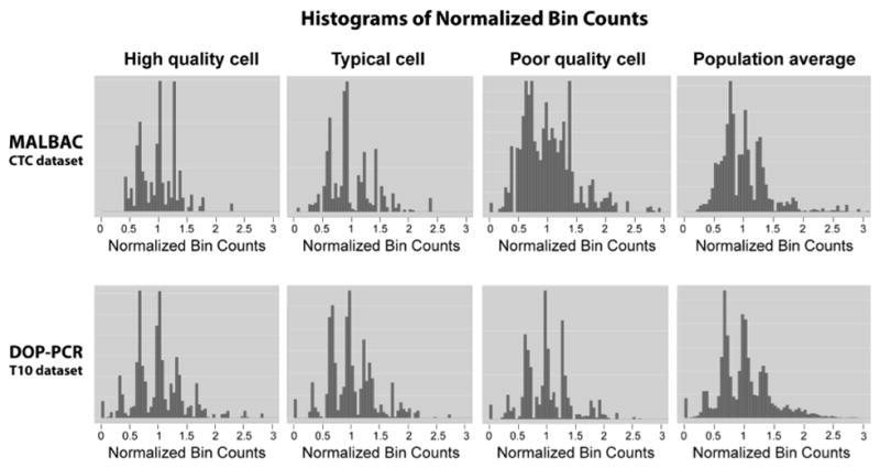
Histograms of normalized bin counts across the CTC and T10 datasets, for a high-, typical-, and poor-quality cell. The rightmost column contains histograms of high quality cell population averages. Distinct peaks are representative of clean data from which accurate copy number calls can be made.

4. Simulation analysis of copy number accuracy

To test the accuracy of the copy number and clustering analysis by Ginkgo, we simulated single cell sequencing of 90 cells with 100 total copy-number events per cell. We modeled the cells after a population comprised of 9 distinct clonal populations, with 10 cells per population (Fig. 5a). We began by generating 3 primary clonal populations by introducing 80 copy-number events compared to the parent diploid cell. Next, for each of the 3 primary clones, we generated 3 subclonal populations by introducing an additional 20 non-overlapping copy-number events to the original clones. Overall, this resulted in 9 distinct subclones belonging to 3 larger clonal populations with a total of 100 CNVs with respect to the human reference genome (hg19).

Figure 5.

(a) Model representation of the 9 distinct subclones generated by simulation of 100 copy number events with respect to the reference. (b) Hierarchical clustering of the 90 samples by Ginkgo. Ginkgo perfectly recovers the underlying subclonal population structure.

The genome positions of CNVs were non-overlapping and generated from a uniform random distribution across the genome. The lengths of CNVs were generated from an exponential distribution with a mean of 5Mb and bounded between the range of 200kb and 20Mb to approximate the CNVs observed in the genuine data. The copy-number state of the CNVs were generated from a Poisson distribution with a mean of 2.5 excluding the value 2.

We generated 10 cells from each of the 9 subclones (90 cells in total) by simulating reads from the subclone reference sequences generated above. For each cell, we simulated 200k, 101bp, single-end reads from the subclone reference sequence using dwgsim (https://github.com/nh13/DWGSIM) (dwgsim –n 101 –z -1 –e .01 –d 1 –r 0 -1 101 -2 0). For each cell, the simulated reads were then mapped to the hg19 human reference genome using the command “bowtie hg19.fa –S –t –m --best –strata” and filtered for only uniquely mappable high scoring reads (quality > 25). The SAM output was then converted to BED format and all 90 cells were uploaded and analyzed directly within Ginkgo with variable length 50kb bins.

Ginkgo is able to accurately reproduce the population structure through hierarchical clustering (Fig. 5b). In addition, we examined Ginkgo’s ability to call CNVs by examining the false negative and false positive rates for all 90 cells at three different read counts (2M, 1.5M, 1M) across three different bin sizes (100kb, 50kb, 25kb) (Supplementary Table 2). We measured Ginkgo to have a 0.15% negative and 0.08% false positive rate excluding those bins that are partially spanned by a copy number alteration. When the entire genome is considered, including partially spanned bins, Ginkgo still has only an ~2% false negative and ~1.2% positive rate. Hence, as expected, errors are almost exclusively concentrated at the boundaries of CNVs where the precise end of the event cannot be determined due to the extremely low coverage available or partially spanning of a bin.

We compared these results to the widely used CNVnator algorithm (http://sv.gersteinlab.org/cnvnator) for bulk sequencing CNV analysis and find that Ginkgo performs CNV calls with higher accuracy (Supplementary Table 2). Furthermore, CNVnator and other bulk sample analysis programs do not attempt to assign integer copy number states, but in this analysis we have measured Ginkgo’s accuracy with this more strict requirement while for CNVnator we could only evaluate if an amplification or deletion had been identified. Ginkgo also has numerous features for evaluating population-wide CNV relationships (heatmaps & hierarchical clusters, multi-sample GC & Lorenz plots, etc) that are also not present in CNVnator or other bulk sample programs that we could not evaluate. Finally, in a practical sense, we also find Ginkgo to be substantially faster than CNVnator, requiring a few hours via a simple web-interface rather than many days in a very difficult to install console program for the 90 cell evaluation.

References

- 1.Shapiro E, Biezuner T, Linnarsson S. Single-cell sequencing-based technologies will revolutionize whole-organism science. Nature reviews. Genetics. 2013;14:618–630. doi: 10.1038/nrg3542. [DOI] [PubMed] [Google Scholar]
- 2.Wigler M. Broad applications of single-cell nucleic acid analysis in biomedical research. Genome Med. 2012;4:79. doi: 10.1186/gm380. [DOI] [PMC free article] [PubMed] [Google Scholar]
- 3.McConnell MJ, et al. Mosaic copy number variation in human neurons. Science. 2013;342:632–637. doi: 10.1126/science.1243472. [DOI] [PMC free article] [PubMed] [Google Scholar]
- 4.Blainey PC. The future is now: single-cell genomics of bacteria and archaea. FEMS Microbiol Rev. 2013;37:407–427. doi: 10.1111/1574-6976.12015. [DOI] [PMC free article] [PubMed] [Google Scholar]
- 5.Wang J, Fan HC, Behr B, Quake SR. Genome-wide single-cell analysis of recombination activity and de novo mutation rates in human sperm. Cell. 2012;150:402–412. doi: 10.1016/j.cell.2012.06.030. [DOI] [PMC free article] [PubMed] [Google Scholar]
- 6.Gundry M, Li W, Maqbool SB, Vijg J. Direct, genome-wide assessment of DNA mutations in single cells. Nucleic Acids Research. 2012;40:2032–2040. doi: 10.1093/nar/gkr949. [DOI] [PMC free article] [PubMed] [Google Scholar]
- 7.Navin N, et al. Tumour evolution inferred by single-cell sequencing. Nature. 2011;472:90–94. doi: 10.1038/nature09807. [DOI] [PMC free article] [PubMed] [Google Scholar]
- 8.Ni XH, et al. Reproducible copy number variation patterns among single circulating tumor cells of lung cancer patients. P Natl Acad Sci USA. 2013;110:21083–21088. doi: 10.1073/pnas.1320659110. [DOI] [PMC free article] [PubMed] [Google Scholar]
- 9.Lu S, et al. Probing meiotic recombination and aneuploidy of single sperm cells by whole-genome sequencing. Science. 2012;338:1627–1630. doi: 10.1126/science.1229112. [DOI] [PMC free article] [PubMed] [Google Scholar]
- 10.Navin N, et al. Inferring tumor progression from genomic heterogeneity. Genome research. 2010;20:68–80. doi: 10.1101/gr.099622.109. [DOI] [PMC free article] [PubMed] [Google Scholar]
- 11.Henrichsen CN, Chaignat E, Reymond A. Copy number variants, diseases and gene expression. Hum Mol Genet. 2009;18:R1–8. doi: 10.1093/hmg/ddp011. [DOI] [PubMed] [Google Scholar]
- 12.Alkan C, Coe BP, Eichler EE. Genome structural variation discovery and genotyping. Nature reviews. Genetics. 2011;12:363–376. doi: 10.1038/nrg2958. [DOI] [PMC free article] [PubMed] [Google Scholar]
- 13.Baslan T, et al. Genome-wide copy number analysis of single cells. Nat Protoc. 2012;7:1024–1041. doi: 10.1038/nprot.2012.039. [DOI] [PMC free article] [PubMed] [Google Scholar]
- 14.Smits SA, Ouverney CC. jsPhyloSVG: a javascript library for visualizing interactive and vector-based phylogenetic trees on the web. PLoS One. 2010;5:e12267. doi: 10.1371/journal.pone.0012267. [DOI] [PMC free article] [PubMed] [Google Scholar]
- 15.Zong C, Lu S, Chapman AR, Xie XS. Genome-wide detection of single-nucleotide and copy-number variations of a single human cell. Science. 2012;338:1622–1626. doi: 10.1126/science.1229164. [DOI] [PMC free article] [PubMed] [Google Scholar]
- 16.Ross MG, et al. Characterizing and measuring bias in sequence data. Genome Biology. 2013;14:R51. doi: 10.1186/gb-2013-14-5-r51. [DOI] [PMC free article] [PubMed] [Google Scholar]
- 17.Navin NE. Cancer genomics: one cell at a time. Genome Biology. 2014;15:452. doi: 10.1186/s13059-014-0452-9. [DOI] [PMC free article] [PubMed] [Google Scholar]
- 18.Cai X, et al. Single-cell, genome-wide sequencing identifies clonal somatic copy-number variation in the human brain. Cell Rep. 2014;8:1280–1289. doi: 10.1016/j.celrep.2014.07.043. [DOI] [PMC free article] [PubMed] [Google Scholar]
- 19.Chen M, et al. Comparison of multiple displacement amplification (MDA) and multiple annealing and looping-based amplification cycles (MALBAC) in single-cell sequencing. PLoS One. 2014;9:e114520. doi: 10.1371/journal.pone.0114520. [DOI] [PMC free article] [PubMed] [Google Scholar]
- 20.de Bourcy CF, et al. A quantitative comparison of single-cell whole genome amplification methods. PLoS One. 2014;9:e105585. doi: 10.1371/journal.pone.0105585. [DOI] [PMC free article] [PubMed] [Google Scholar]
Associated Data
This section collects any data citations, data availability statements, or supplementary materials included in this article.