Incorporating Local Land Use Regression And Satellite Aerosol Optical Depth In A Hybrid Model Of Spatio-Temporal PM_2.5 Exposures In The Mid-Atlantic States

Abstract

Satellite-derived Aerosol Optical Depth (AOD) measurements have the potential to provide spatio-temporally resolved predictions of both long and short term exposures, but previous studies have generally shown moderate predictive power and lacked detailed high spatio-temporal resolution predictions across large domains. We aimed at extending our previous work by validating our model in another region with different geographical and metrological characteristics, and incorporating fine scale land use regression and nonrandom missingness to better predict PM_2.5 concentrations for days with or without satellite AOD measures. We start by calibrating AOD data for 2000–2008 across the Mid-Atlantic. We used mixed models regressing PM_2.5 measurements against day-specific random intercepts, and fixed and random AOD and temperature slopes. We used inverse probability weighting to account for nonrandom missingness of AOD, nested regions within days to capture spatial variation in the daily calibration, and introduced a penalization method that reduces the dimensionality of the large number of spatial and temporal predictors without selecting different predictors in different locations. We then take advantage of the association between grid-cell specific AOD values and PM_2.5 monitoring data, together with associations between AOD values in neighboring grid cells to develop grid cell predictions when AOD is missing. Finally to get local predictions (at the resolution of 50m), we regressed the residuals from the predictions for each monitor from these previous steps against the local land use variables specific for each monitor. “Out-of-sample” ten-fold-cross validation was used to quantify the accuracy of our predictions at each step. For all days without AOD values, model performance was excellent (mean “out-of-sample” R²=0.81, year-to-year variation 0.79–0.84). Upon removal of outliers in the PM_2.5 monitoring data, the results of the cross validation procedure was even better (overall mean ”out of sample” R² of 0.85). Further, cross validation results revealed no bias in the predicted concentrations (Slope of observed vs. predicted = 0.97–1.01). Our model allows one to reliably assess short-term and long-term human exposures in order to investigate both the acute and effects of ambient particles, respectively.

Graphical abstract

1. Introduction

Fine Particulate Matter (PM) is a complex mixture of particles primarily composed of sulfate (SO4), nitrates (NO3), ammonium (NH4), elemental carbon (EC), organic compounds (OC), and various metals (1). PM originates from a variety of stationary and mobile sources and may be directly emitted (primary emissions) or formed in the atmosphere by transformation of gaseous emissions (secondary emissions).

Multiple studies have demonstrated the association between both short and long term exposures to PM_2.5 (particulate matter that is 2.5 micrometers or smaller in diameter) and adverse health effects. Multiple health effects have been shown including asthma (2, 3), cardiovascular problems (4, 5), respiratory infections (4, 6), mortality (7–9) and lower birth weights (10–13). This adverse association has been demonstrated for a wide range of concentration levels in various regions of the world, yet an important limitation of most previous studies is that they all rely upon a limited number of PM_2.5 monitoring sites placed within the study area. Because these sites do not measure individual-specific exposure, this approach introduces exposure error, and likely biases the effect estimates downward (14). In addition, a key limitation is that they are unable to produce estimates in locations without monitors nearby, and people who live in more densely populated areas are unlikely to be representative of those who do not.

Land use (LU) regression exposure models are commonly used in health studies, yet since the LU terms are generally not time varying, their temporal resolution tends to be limited, and based on the spatial resolution of the available PM_2.5 monitoring network (15–18). Land use terms capture traffic and point sources, but spatial smoothing is required to capture variation in secondary aerosols. In addition the coefficients of the land use terms are determined by land patterns around ambient monitoring stations, whose locations may be non-representative of LU in general in the U.S. These same locations drive the spatial smoothing of LU. Hence extrapolation of predictions from these models to other areas involves error and may yield biased estimates of exposure. A further limitation of LU models is that they do not provide predictions for acute (short term exposure) studies.

Satellite data in general and particularly satellite derived aerosol optical depth (AOD) data provides another important tool for monitoring aerosols due to its large spatial coverage and reliable repeated physical measurements, particularly for areas and exposure scenarios where surface PM_2.5 monitors are not available (19–22). We have recently published a novel hybrid method to predict daily temporally and spatially resolved PM_2.5 across New-England for the years 2000–2008 (22). These predictions, which are based on land use regression plus a daily calibration of PM_2.5 ground measurements and MODIS (Moderate Resolution Imaging Spectroradiometer) satellite AOD, allow for the prediction of daily PM_2.5 concentration levels at the resolution of a 10×10 km spatial grid. Model performance was excellent, even for days having no AOD data. Ten-fold out-of-sample cross validation yielded a mean “out-of-sample” R² of 0.81. By averaging our estimated daily exposures at each location we can generated long term exposures. This enabled us to generate both the short term and long term effects of ambient particles, respectively. We have used those estimates to assess the association of PM_2.5 with both hospital admissions in New England and birth weight for all births in Massachusetts.

Although our model performance was excellent, it is important to validate it in another region with different geographical and meteorological characteristics. In addition, there is room for further methodological improvements in our model. For example, AOD data availability is much greater in the summer periods compared to the winter period. This is mostly due to heavily clouded days or snow cover in winter periods which results in missing AOD data. This non-random missingness of AOD readings could cause selection bias, which could in turn negatively affect predictive performance. Also, treating large areas, such as the Mid-Atlantic region of the United States, as one region can add additional bias since there may be geographic variations in the daily calibration between PM_2.5 and AOD. Finally, land use regressions typically start with a large number of land use terms, and choose a subset by methods that risk overfitting and result in different variable choices in different models. In addition, space time interactions are rarely accommodated.

Thus in this paper we extend our previous work in New-England by upgrading and validating our model using the Mid-Atlantic area in the eastern part of the USA. Specifically, we developed and validated models to predict daily PM_2.5 at a 10×10 km resolution and at local addresses across the Mid-Atlantic region for the years 2000–2008. We updated the model by adding inverse probability weights to account for missing days when AOD cannot be included in the primary analysis due to its missingness. We divided the Mid-Atlantic area into 7 regions based on the geography of the region and incorporate nested day-specific calibration of the AOD-PM_2.5 relation by region. Additionally we developed an approach that allows us to include all land use and meteorological variables and their interactions, with appropriate shrinkage back to their mean effect by category (e.g. land use, temporal and interaction).

2. Material and Methods

2.1 Study domain

The spatial domain of our study included the Mid-Atlantic region in the USA comprising the states of Delaware, Maryland, New Jersey, Pennsylvania, Washington D.C., Virginia, New York, West Virginia, (Figure 1). They cover an area of 495,486 km² and have a population of 57,303,316 (23). The Mid-Atlantic States include some of the largest metropolitan areas in the USA including among others: Baltimore, Washington, Philadelphia, New York, Newark and Pittsburgh.

Figure 1.

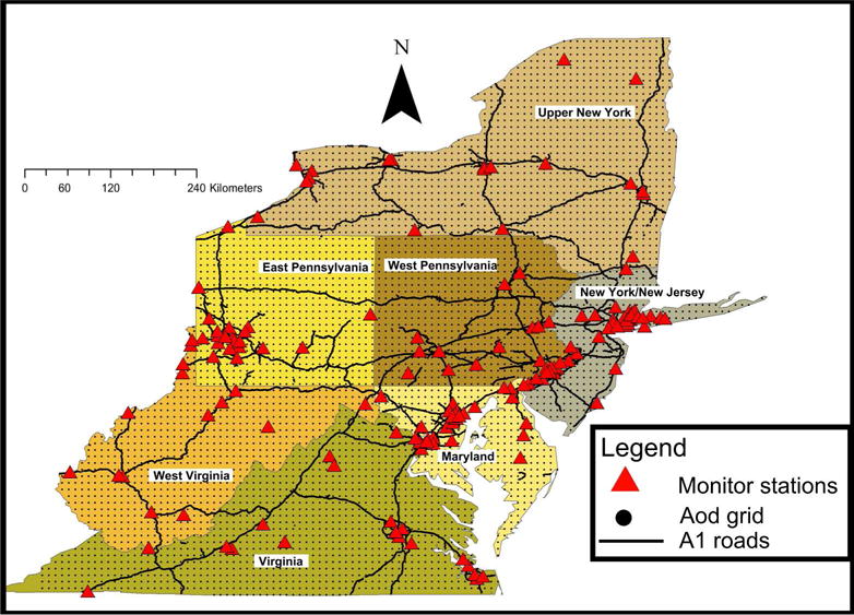
Map of the study area showing the full AOD grid, the regions and all PM_2.5 monitor station across the Mid-Atlantic.

2.2 AOD Data

The Moderate Resolution Imaging Spectroradiometer (MODIS) sits aboard the Earth Observing System (EOS) satellites (24, 25). The Terra and Aqua satellites were launched in December 18, 1999 and in May 4^th, 2002 respectively. The satellites are polar-orbiting satellites and operate at an altitude of approximately 700 km. Their sensors scan the swath of 2330 km (cross-track) by 10 km (along-track at nadir). For Terra, the local equatorial crossing time is approximately 10:30 A.M. while for Aqua it is 13:30 P.M. Both satellites perform measurements in the visible to thermal infrared spectrum region. One of the fundamental aerosol products from MODIS is spectral AOD (also known as Aerosol Optical Thickness-AOT). MODIS level 2 files are produced daily, and represent the first level of MODIS aerosol retrieval. Bands 1 through 7 are devised to study aerosols, and a number of other bands help with cloud rejection and other screening procedures. The aerosol algorithm relies on calibrated, geo-located reflectance Level 1B data (25).

More details about MODIS satellite data have been reported (26, 27). Daily data are freely available online through the NASA website (28). For the analysis presented here daily MODIS level 2 files from the Terra satellite for the years 2000–2008 were used at the spatial resolution of 10 km × 10 km at nadir. MODIS AOD pixel centroids constantly shift daily between orbits, thus we created a fixed 10×10 km grid. Daily values of AOD were assigned to the grid cell where the AOD retrieval’s centroid was located. Aqua satellite data was not used since it was only launched late 2002. Although there are other satellites that measure AOD, the MODIS satellite was used since it is the most validated (using AERONET), accessible and accurate dataset available today (Remer et al. 2005).

2.3 Monitoring data

Data for daily PM_2.5 mass concentrations across the Mid-Atlantic region (see Figure 1) for the years 2000–2008 were obtained from the US Environmental Protection Agency (EPA) Air Quality System (AQS) database as well as the IMPROVE (Interagency Monitoring of Protected Visual Environments) network. IMPROVE monitor sites are located in national parks and wilderness areas while EPA monitoring sites are located across the Mid-Atlantic including urban areas such as New York city, Washington DC, Baltimore etc. There were 161 monitors with unique locations operating in the Mid-Atlantic during the study period. The Mean PM_2.5 across the Mid Atlantic during the study period was 13.59 μg/m³ with a standard deviation of 8.52 μg/m³ and a 10.10 μg/m³ interquartile range (IQR).

2.4 Spatial Predictors of PM_2.5

The available spatial predictors for our model were percent of open space, population density, elevation, traffic density, PM_2.5 point emissions and area-source PM_2.5 emissions. Percent of open spaces: Percent of open spaces data were obtained through the 2001 national land cover data (NLCD) multi-resolution land characteristics consortium (MRLC) (30). Data were obtained as raster files with 30 m cell size. Percent of open space included all areas such as parks, forestry, golf courses, and vegetation planted in developed settings for recreation, erosion control, or aesthetic purposes.

Elevation

Elevation data were obtained through the national elevation dataset (NED) (31). NED is distributed by the U.S. Geological Survey (USGS) and provides seamless raster elevation data of the conterminous United States. The NED is released in geographic coordinates at a resolution of 1 arc sec.

Traffic Density

Road data were obtained through the US census 2000 topologically integrated geographic encoding and referencing system (TIGER)(32). We calculated the total A1 road length (class 1 roads that are hard surface highways including Interstate and U.S. numbered highways, primary State routes, and all controlled access highways) across the Mid-Atlantic. The A1 roads were intersected with the 10×10 grid cell and the resulting attribute tables contained the density of all A1 road segment lengths in the 10 km grid.

PM _2.5 point emissions

PM_2.5 point emissions were obtained through the 2005 USEPA National Emissions Inventory (NEI) facility emissions report (33). Because the distributions of point source emissions were highly right-skewed, the emission values were log transformed. Locations reporting zero emissions within the appropriate grid were assigned a value of one half of the minimum value among all monitoring locations.

Area-source PM_2.5 emissions

Area-source PM_2.5 emissions data were obtained through the 2005 USEPA -NEI tiered emissions reports (33), which provide estimates of total area-source emissions of PM_2.5 by county and year. Intersecting source emission areas for each 10×10 km grid were weight averaged and similarly log-transformed.

2.5 Temporal Predictors of PM_2.5

Meteorologic data

All meteorological variables used in the analysis (temperature, wind speed, visibility and relative humidity) were obtained through the national climatic data center (NCDC) (34). Only continuous operating stations with daily data running from 2000–2008 were used (26 stations). Grid cells were matched to the closest weather station for meteorological variables.

2.6 Statistical Methods

All modeling was done using the R statistical software version 2.15.0 and SAS (Statistical Analysis System) version 9.3.

In our prediction models we accommodate the two most common data types in health studies: small area (census areas, postal code areas etc…) geocoded data (SAGD) and residence-specific latitude and longitude geocoded data (RGD). When using SAGD we use only our grid cell model (at a 10×10km spatial resolution) while when RGD are available, we use a local land use regression component.

To estimate PM_2.5 concentrations in each grid cell on each day we run the prediction process in four stages. We first summarize the stages here before presenting the regression model used at each stage. The stage 1 model calibrates the AOD grid-level observations to the PM_2.5 monitoring data collected within 10km of an AOD reading by regressing PM2.5 monitoring data on AOD values and other predictors. Because the relationship between AOD and PM_2.5 varies day to day (due to differences in mixing height, relative humidity, particle composition, vertical profiles etc), this calibration is performed on a daily basis. Further, because the mid-Atlantic area of the US is relatively large and this PM-AOD relationship can vary spatially, we partitioned mid-Atlantic study area is divided into seven regions and assumed this calibration additionally varied by region. In stage 2 we predict PM_2.5 concentrations in grid cells without monitors but with available AOD measurements using the stage 1 fit. This is achieved by simply applying the estimated prediction equation obtained from the model fit in stage 1 to these additional AOD values. In stage 3, to estimate PM_2.5 concentrations in cells where no AOD data is missing, we fit a model that uses predicted levels of PM_2.5 from stage 2 and spatial associations among PM_2.5 levels on a given day to estimate daily PM_2.5 in cells not having AOD on a given day.

These first three steps are applied to the data at the 10 km × 10km grid cell level. To calculate the local PM_2.5 concentrations in studies using RGD, we take the residuals of the stage 3 model at each monitoring site and regress them against local (50 m buffer) LU terms at each monitor. The fitted values from this local regression stage are then added back to the grid-level predictions obtained in Stage 3 to produce residence-level predictions.

Stage 1

The base model (stage 1) consists of a mixed model that regresses PM_2.5 monitoring data on grid-level AOD values, temperature, and other land-use regression terms. To perform this PM_2.5-AOD calibration on a day-specific and region-specific basis, the coefficients in this model were assumed to be random effects, meaning these terms vary across the population of days and regions according to some random distribution. These day-region terms are nested, such that a coefficient for a given region-day combination varies randomly around an overall coefficient specific to that day, which itself varies across the entire population of days in which AOD is available. This structure is assumed for the intercepts, AOD slopes, and temperature slopes in the model.

In addition, a moderately large number of additional spatial, temporal (daily), and spatio-temporal predictors are included as predictors in the PM_2.5 model. Because use of many predictors can lead to overfitting and lack of precision of the resulting estimates, we allow the effect of each variable to be unique but shrink groups of these effects back to a common mean, which represents a form of regularization, or penalization, of the resulting coefficients that can stabilize estimation and avoid overfitting. We group these coefficients into the spatial terms, the temporal terms, and the spatio-temporal terms, and shrink each set of coefficients back towards a mean for each of these three groups of variables. The shrinkage is accomplished by treating the coefficient of each variable as a random slope, and shrinking coefficient back to the group-specific mean. We standardize each of these variables to have standard deviation 1. Therefore, this mean coefficient, represented in the model as a fixed effect, represents the mean effect on PM_2.5, averaged across the variables in that group of covariates. In the final model we leave only the random slopes for the spatio-temporal terms since the separate spatial and temporal terms have a relatively small number of covariates and were not statistically significant. However, we present the full model here for cases in which more predictors are candidates for inclusion in the model. Taken all together, the first stage of the model can be written as:

$${\mathrm{PM}}_{\mathrm{ij}}=(\mathrm{\alpha }+{\mathrm{u}}_{\mathrm{j}+}{\mathrm{g}}_{\mathrm{j}(\text{reg})})+({\mathrm{\beta }}_1+{\mathrm{v}}_{\mathrm{j}}+{\mathrm{h}}_{\mathrm{j}(\text{reg})}){\text{AOD}}_{\mathrm{ij}}+({\mathrm{\beta }}_2+{\mathrm{k}}_{\mathrm{j}}){\text{Temperature}}_{\mathrm{ij}}+{\sum }_{m=1}^3{\gamma }_{1m}{X}_{1mi}+{\sum }_{m=1}^6{\gamma }_{2m}{X}_{2mj}+{\sum }_{m=1}^{18}{\gamma }_{3m}{X}_{3\mathit{mij}}+{\mathrm{\epsilon }}_{\mathrm{ij}}$$

$$({\mathrm{u}}_{\mathrm{j}}{\mathrm{v}}_{\mathrm{j}}{\mathrm{k}}_{\mathrm{j}})~N[(000),\sum ]$$

$$({\mathrm{g}}_{\mathrm{j}(\text{reg})},{\mathrm{h}}_{\mathrm{j}(\text{reg})})~\mathrm{N}[(00),{\sum }_{\text{REG}}]$$

$$({\gamma }_{11,\dots }{\gamma }_{1,3})~\mathrm{N}[{\gamma }_1,{{\mathrm{\sigma }}^2}_1]$$

$$({\gamma }_{21,\dots }{\gamma }_{2,6})~\mathrm{N}[{\gamma }_2,{{\mathrm{\sigma }}^2}_2]$$

$$({\gamma }_{31,\dots }{\gamma }_{3,18})~\mathrm{N}[{\gamma }_3,{{\mathrm{\sigma }}^2}_3]$$

where PM_ij is the measured PM_2.5 concentration at a spatial site i on a day j; α and u_j are the fixed and random day-specific intercepts, respectively, AOD_ij is the AOD value in the grid cell corresponding to site i on a day j; β₁ and v_j are the fixed and random day-specific slopes, respectively. Temperature_ij is the temperature value in the grid the cell corresponding to site i on a day j (β₂ and k_j are the fixed and random slopes for temperature).X_1mi is the value of the mth spatial predictor at site i, X_2mj is the value of the mth temporal predictor on day j, and X_3mij is the value of the mth spatial-temporal predictor at site i on day j. g_j(reg) and h_j(reg) are the daily random intercepts and AOD slopes specific to each study area region. Here, we assume Σ is a 3 × 3 diagonal matrix with diagonal elements σ²_u, σ²_v, σ²_k and Σ_REG is a 2 × 2 diagonal matrix with diagonal elements σ²_g, σ²_h.

Second, to accommodate the fact that daily AOD data missingness is not random, the first-stage model incorporated inverse probability weighting (IPW) to potentially avoid bias in the regression coefficient estimates and thus in the resulting predictions. This approach effectively up-weights dates and grid cells which are under-represented due to a large degree of missing data. To obtain the weights that account for the non-random missingness in AOD values, we fit the following model for the probability (p) of observing an AOD value in cell i on day j, fit separately from the stage 1 model:

$$\mathit{ln}(\frac{\widehat{\mathit{p}}}{1-\widehat{\mathit{p}}})={\mathrm{\beta }}_0+{\mathrm{\beta }}_1{\text{Elevation}}_{\mathrm{i}}+{\mathrm{\beta }}_2\text{Sea Line}{\text{Pressure}}_{\mathrm{ij}}+{\mathrm{\beta }}_3{\text{Temperature}}_{\mathrm{ij}}+\text{Month},$$

where (p) is the probability of AOD availability on each day in each grid cell in each year. We then use the inverse probability weights in the above mixed model. There were no observations which had a disproportionate influence in the yearly models.

$$\mathit{IPW}=(\frac{1}{\widehat{p}})$$

The stage 1 model was fit to data from each year (2000–2008) separately. To validate the first stage of our model, the dataset was repeatedly randomly divided into 90% and 10% splits. Predictions for the held-out 10% of the data were made from the model fit of the remaining 90% of the data. This “out of sample” process was repeated ten times and cross-validated (CV) R² values were computed. To check for bias we regressed the measured PM_2.5 values against the predicted values in each held out site on each day. Overall temporal R² was calculated by regressing Delta PM against Delta predicted where: Delta PM is the difference between the observed PM_2.5 at a given site on a given day and the annual mean PM_2.5 at that location, and Delta predicted is defined similarly for the predicted values generated from the model. Overall spatial R² was calculated by regressing the annual mean PM_2.5 at a given site against the annual mean predicted PM_2.5 at that location.

We also tested the model performance (CV) for a test year (2001) without including AOD (only MET and LU variables were regressed against PM_2.5 with a random intercept by date and a random slope for temperature) and by using a traditional kriging method.

Stage 2

The next stage (stage 2), uses the fit of the stage 1 model to predict a PM_2.5 concentration for each day and grid at which we have an observed AOD value. This resulted in yearly datasets with PM_2.5 prediction for all day-AOD cell available combinations yet still no predictions in day-cell combinations with missing AOD data.

Stage 3

In stage 3 of the model, we estimated daily PM_2.5 concentration levels for all grid cells in the study domain for days when AOD data were unavailable. Using the PM_2.5 predictions obtained from the first stage of the model as the response, we fit a model containing a smooth function of latitude and longitude (of the grid cell centroid) and a random intercept for each cell. This is similar to universal kriging, extended to include the mean of the PM_2.5 monitors on that day (the average PM_2.5 concentrations measured at all the available PM_2.5 monitors in the region on each day) and random cell-specific slope. To allow for temporal variations in the spatial correlation, a separate spatial surface was fit for each two-month period of each year. Using this method provides additional information about the concentration in the missing grid cells that simple kriging would not. Specifically this stage (stage 3) fits the following semiparametric regression model:

$${\text{PredPM}}_{\mathrm{ij}}=(\mathrm{\alpha }+{\mathrm{u}}_{\mathrm{i}})+({\mathrm{\beta }}_1+{\mathrm{v}}_{\mathrm{i}}){\mathrm{MPM}}_{\mathrm{j}}+\text{Smooth}(\mathrm{X},\mathrm{Y}){}_{\mathrm{k}(\mathrm{j})}+{\mathrm{\epsilon }}_{\mathrm{ij}},$$

$$({\mathrm{u}}_{\mathrm{j}}{\mathrm{v}}_{\mathrm{j}})~[(\mathbf{0}\mathbf{0}),{\Omega }_{\beta }]$$

where PredPM_ij is the predicted PM_2.5 concentration at a spatial site i on a day j from the 2^nd stage model; MPM_j is the mean PM in the relevant region on a day j; α and u_i are the fixed and grid-cell specific random intercepts, respectively; β₁ and v_i are the fixed and grid-cell specific random slopes, respectively. The smooth X,Y is a thin plate spline fit to the latitude and longitude, k(j) denotes the two-month period in which day j falls (that is, a separate spatial smooth was fit for each two-month period).

To estimate the goodness of fit, we dropped “all observations” at a particular site each time (ten times and taking out 10% of specific monitors). Then the cross validation was performed against PM_2.5 stations that were left out altogether from the analysis. This “out of sample” process was repeated ten times and CV R² values were computed.

Stage 4

Finally, for cases in which health outcomes are resolved to the specific longitude and latitude for a given study subject residence, we fit a local PM stage (stage 4) that takes the residuals constructed by taking the difference between a given monitored PM_2.5 concentration and the 10km × 10km grid prediction from Stage 3 for the grid in which that monitor is located, and regresses these residuals on location-specific predictors of pollution. Specifically, we fit the following model

$$\mathit{Resid}P{M}_{ij}=f_1({\mathit{\text{Traffic Density}}}_i,{\mathit{\text{Population Density}}}_i)+f_2({\mathit{\text{Elevation}}}_i)+f_3({\mathit{\text{Percent Urban}}}_i)+f_4(\mathit{\text{Distance to}}A1{\mathit{\text{roads}}}_i)++f_5({\mathit{\text{Distance to Point emissions}}}_i)+{\epsilon }_{\mathit{ij}}$$

where ResidPM_ij is the residual at a spatial monitor site i on day j; f₁ denotes a penalized spline for an interaction between traffic density and population density; f₂–f₅ denote (potentially nonlinear) effects of elevation, percent urbanicity, distance to A1 road, and distance to point emissions, respectively, on these residuals, and ε_ij is the error. In contrast to stage 1, where land use terms were grid cell averages, for this model land use terms were all computed for a 50 m radius about the monitor, to capture local effects. The models used cubic penalized splines within a mixed model framework, as implemented in the GAMM function in R. We used the default amount of smoothing for each nonlinear term in the model.

We calculated prediction errors for the spatial components in each stage (to be comparable to all previous available model which don’t have daily measurements) by subtracting retained observations from the model predictions. We estimated the model prediction precision by taking the square root of the mean squared prediction errors (RMSPE) (35).

3. Results

Figure 2 presents a scatter plot of the AOD-PM_2.5 relationship before (Fig. 2a) and after (Fig. 2b) the stage 1 calibration showing the significant fit improvement gained by calibrating with our stage 1 model.

Figure 2.

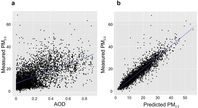
A scatter map of the AOD-PM relationship before and after the calibration.

Table 1 presents the results from the stage 1 analysis. The yearly models all presented very good out-of-sample predictive performance for each year and the entire study period, with a mean out of sample R² of 0.81 (year to year variation 0.76–0.86), and as expected a highly significant association between PM _2.5 and the main explanatory variable AOD (Table 1).

Table 1.

Prediction accuracy: Ten-fold cross validated R² for PM_2.5 stage 1 predictions (Calibration stage for 2000–2008).

Yearly Dataset	CV R2	Intercepta	Slope a	CV R2Spatial	CV R2Temporal	RMSPE b
2000	0.83	0.23 ± 0.10	0.98 ± 0.01	0.73	0.84	1.57 μg/m3
2001	0.81	0.42 ± 0.09	0.97 ± 0.01	0.69	0.82	1.35 μg/m3
2002	0.79	0.52 ± 0.11	0.97 ± 0.01	0.77	0.79	1.30 μg/m3
2003	0.86	− 0.15 ± 0.10	1.01 ± 0.01	0.74	0.87	1.50 μg/m3
2004	0.81	0.19 ± 0.10	0.99 ± 0.01	0.70	0.82	1.50 μg/m3
2005	0.78	− 0.11 ± 0.12	1.01 ± 0.01	0.69	0.80	1.70 μg/m3
2006	0.84	0.26 ± 0.09	0.98 ± 0.01	0.76	0.85	1.22 μg/m3
2007	0.82	0.06 ± 0.09	1.00 ± 0.01	0.82	0.82	1.08 μg/m3
2008	0.76	0.01 ± 0.11	1.00 ± 0.01	0.74	0.76	1.20 μg/m3
Mean 2000–2008	0.81			0.74	0.82	1.38 μg/m3

^aPresented as parameter estimate ± SE from linear regression of held out observations versus predictions.

^bRoot of the mean squared prediction errors.

In addition the stage 1 results revealed that adding the IPW in the model greatly reduced the bias in our cross validation results (Slope of observed vs. predicted = 0.97–1.01).

The spatial and temporal out of sample results also presented very good fits to the held out data (Table 1): For the temporal model the mean out of sample R² was 0.82 (year to year variation 0.76–0.87) and for the spatial model the mean out of sample R² was 0.74 (year to year variation 0.69–0.82).

The results for the 2001 test models excluding AOD, showed that using standard LU regression models (LU+MET) results in much lower CV predictive power (R2=0.67 compared to 0.81 in our AOD models). Using traditional Kriging methods our predictive R² was even lower (0.53). These results indicate that by using the AOD measurements we can improve our model fit quite significantly. The results of the 2001 test model without the weights revealed a R² of 0.79 which is almost 2% less than the model with the weights. Also the bias increases a bit without the weights (slope of 0.96 vs 0.97 with the weights).

The stage 3 models are presented in Table 2. All models performed well with a mean out of sample R² of 0.81 (year to year variation 0.78–0.85), which is relatively high considering that these were days with neither ground PM data nor satellite AOD data in the grid cells being predicted. Again the spatial and temporal out of sample results were very good (Table 2): For the temporal model the mean out of sample R² was 0.83 (year to year variation 0.79–0.85) and for the spatial model the mean out of sample was 0.73 (year to year variation 0.68–0.77).

Table 2.

Prediction accuracy: Ten-folds cross validated R² for Stage3 PM_2.5 predictions (Final prediction model including locations without AOD for 2000–2008).

Yearly Dataset	CV R2	CV R2Spatial	CV R2Temporal	RMSPEa
2000	0.79	0.76	0.79	1.31 μg/m3
2001	0.83	0.80	0.83	1.22 μg/m3
2002	0.85	0.72	0.85	1.17 μg/m3
2003	0.82	0.80	0.82	1.05 μg/m3
2004	0.80	0.75	0.81	1.14 μg/m3
2005	0.80	0.83	0.80	1.13 μg/m3
2006	0.83	0.80	0.84	1.04 μg/m3
2007	0.83	0.80	0.83	0.88 μg/m3
2008	0.78	0.80	0.78	0.88 μg/m3
Mean 2000–2008	0.81	0.78	0.82	1.09 μg/m3

^aRoot of the mean squared prediction errors.

Both the stage 1 and stage 3 models yielded very small predictions errors (RMSPE-Root of the mean squared prediction errors) −1.09 [μg/m3 and 1.38 [μg/m3 respectively, indicating a strong model performance.

Figure 3 shows the spatial pattern of predicted PM_2.5 concentrations from the AOD models, averaged over the entire study period. Mean predicted PM_2.5 concentrations range from 6.48 μg/m³ to 20.80 μg/m³ showing a good range of variability for our model. As expected, predicted PM_2.5 concentrations are higher in urban areas such as New York etc. compared to rural areas such as in upper New York. Increased concentrations along major interstate highways are also clear.

Figure 3.

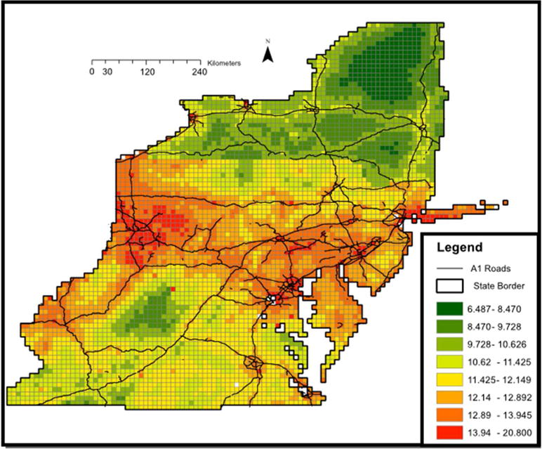
Mean PM_2.5 concentrations in each 10×10 km grid during the entire modeling period (2000–2008) predicted by the AOD models.

By incorporating the local stage (stage 4) we see an increase of 1.9% across all years in mean prediction performance (R²) of the model (compared to the without the local PM stage).

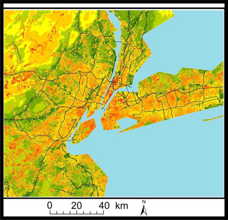
Figure 4 shows the difference of the estimated local pollution (stage 4) from the average PM_2.5 concentrations at a very fine resolution (200×200m). Figure 4a presents the Baltimore Metropolitan area while figure 4b presents the city of New York.

Figure 4.

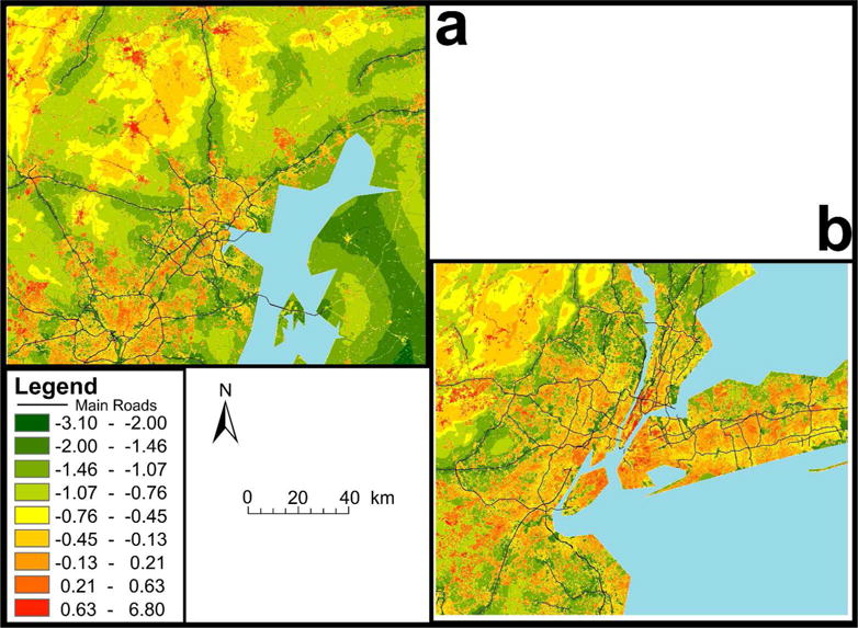
The difference of the estimated local pollution from the average overall annual PM_2.5 concentrations at a very fine resolution (200×200m). Figure 4a presents the Baltimore Metropolitan area while figure 4b presents the city of New York.

4. Discussion

In this paper we examined the relationship between PM_2.5 ground measurements and MODIS AOD data in the Mid Atlantic during the period 2000–2008. This study is an extension of our previous study (22) which we wanted to validate in a different region with different geographic and climatic characteristics. In addition, in the new model we introduce some significant methodological improvements in a few key areas. First, by adding IPW into the first stage calibration, we addressed the issue of selection bias. To account for the varying region characteristics (since the Mid-Atlantic area is a very large area) we divided the Mid-Atlantic into 7 regions and incorporate them as nested regions within days in the model. This allowed us to better address the different spatial-temporal individual characteristics of each separate region and resulted in better predictive performance. Also importantly, we improved on how the different LU and MET (Meteorologic) variables were treated in the model by developing aggregate LU and MET variables (and all their interactions) combining all available LU/MET variables which allow us to include all available spatial and temporal predictors, and shrink them back toward their respective aggregates, instead of stepwise approaches. This helped eliminate the problems of only choosing a subset of available LU/MET terms (often decided subjectively by different researchers) and also helped improve prediction performance.

It is important to emphasize that the predictions of our models perform significantly better than other prediction models which assumed that the relationship between PM_2.5 and MODIS AOD data remains constant over time and much better than models using LU regression alone (16, 36–38). The use of daily measurements of AOD (as opposed to other models) allows better assessment of space time interactions than models that only have spatially resolved time invariant LU terms, since we have actual daily spatial measurements that can show differences in short term particle concentrations between grid cells. This allows us to use the model to make predictions for studies of the acute effects (short term) of air pollution as well as chronic (long term) effects, as well as for studies that attempt to capture both effects.

Multiple studies in recent years have presented models predicting PM_2.5 including some that have established quantitative relationships between satellite-derived AOD and PM_2.5 (35, 39–41). However, all these previous models present either moderate predictive power, or lack detailed high spatial and temporal resolution predictions across large domains. For example, Yanosky and colleagues (35) developed PM_2.5 models which included smooth spatial and regression terms of GIS and meteorological predictors. The predictive performance was good (CV R² 0.77−0.69) and their model only generates monthly predictions. Our model in comparison generates daily predictions with a higher predicative performance (CV R² 0.79–0.84).

It is important to note that we noticed a small group of outliers in our data with extremely high PM_2.5 values corresponding to days with low AOD values. Upon close investigation of these outliers we found that they were are all centered around the major Mid-Atlantic Highway (the I-95) where the relatively coarse 10×10km grid cell for AOD cannot always capture highly polluted days around the highway. The results of the cross validation results without these outliers are much better (overall mean out of sample R² of 0.85 vs. 0.82 with the outliers). On most days, our model performs well in these locations, and we speculate these outlier days are due to a low level inversion, which our model does not capture. We will try to address this in the future by obtaining and incorporating the height of the boundary layer data into our models.

Our model could be applied in various disciplines, particularly in epidemiology. Our PM_2.5 exposure model allows us to gain spatial resolution in the acute effects and an assessment of long-term effects in the entire population, rather than a selective sample from urban locations as commonly done in current epidemiological studies. Studies looking into the association between PM _2.5 and mortality, reduced birth weight etc. thus could greatly benefit from our models for both chronic and acute effects.

The main limitation of the present study is the relatively coarse spatial resolution of 10 × 10 km obtained through the MODIS satellite. However, as satellite remote sensing evolves, higher spatial resolution data, e.g., 1 × 1 km, should become available which will further reduce exposure error. We address this limitation somewhat by using our fourth stage model (the local PM step for RGD) where we generate local predictions at individual addresses. Another limitation is the lack of data on the composition of AOD particles. Future analysis may allow us to develop exposure estimation for specific PM components and other pollutants.

In summary, we have clearly demonstrated how AOD can be used reliably to predict daily PM_2.5 mass concentrations in the Mid-Atlantic area, validating our previous model in another area. We have also shown how our model improves further by adding methodological improvements, allowing us to address some of the shortcoming of the first iteration of the model. Importantly, our model allows us to assess short term and long term human exposures in order to investigate both the acute and effects of ambient particles, respectively.

References

- 1.Seinfeld JH, Pandis SN. Atmospheric Chemistry and Physics: From Air Pollution to Climate Change. Wiley-Interscience; 1998. [Google Scholar]
- 2.Sheppard L, Levy D, Norris G, Larson TV, Koenig JQ. Effects of ambient air pollution on nonelderly asthma hospital admissions in Seattle, Washington, 1987–1994. Epidemiology. 1999:23–30. [PubMed] [Google Scholar]
- 3.Schwartz J, Slater D, Larson TV, Pierson WE, Koenig JQ. Particulate air pollution and hospital emergency room visits for asthma in Seattle. American Journal of Respiratory and Critical Care Medicine. 1993;147:826–831. doi: 10.1164/ajrccm/147.4.826. [DOI] [PubMed] [Google Scholar]
- 4.Kloog I, Coull BA, Zanobetti A, Koutrakis P, Schwartz JD. Acute and chronic effects of particles on hospital admissions in new-England. PloS one. 2012;7:e34664. doi: 10.1371/journal.pone.0034664. [DOI] [PMC free article] [PubMed] [Google Scholar]
- 5.Wellenius GA, Bateson TF, Mittleman MA, Schwartz J. Particulate air pollution and the rate of hospitalization for congestive heart failure among medicare beneficiaries in Pittsburgh, Pennsylvania. Am J Epidemiol. 2005;161:1030–6. doi: 10.1093/aje/kwi135. [DOI] [PMC free article] [PubMed] [Google Scholar]
- 6.Zanobetti A, Franklin M, Koutrakis P, Schwartz J. Fine particulate air pollution and its components in association with cause-specific emergency admissions. Environ Health. 2009;8:58. doi: 10.1186/1476-069X-8-58. [DOI] [PMC free article] [PubMed] [Google Scholar]
- 7.Dockery D, Pope C, Xu X, Spengler J, Ware J, Fay M, Ferris B, Speizer F. An association between air pollution and mortality in six US cities. The New England journal of medicine. 1993;329:1753–1759. doi: 10.1056/NEJM199312093292401. [DOI] [PubMed] [Google Scholar]
- 8.Franklin M, Zeka A, Schwartz J. Association between PM2.5 and all-cause and specific-cause mortality in 27 US communities. Journal of Exposure Science and Environmental Epidemiology. 2006;17:279–287. doi: 10.1038/sj.jes.7500530. [DOI] [PubMed] [Google Scholar]
- 9.Pope C, III, Burnett R, Thun M, Calle E, Krewski D, Ito K, Thurston G. Lung cancer, cardiopulmonary mortality, and long-term exposure to fine particulate air pollution. Jama. 2002;287:1132–1141. doi: 10.1001/jama.287.9.1132. [DOI] [PMC free article] [PubMed] [Google Scholar]
- 10.Bonzini M, Carugno M, Grillo P, Mensi C, Bertazzi PA, Pesatori AC. Impact of ambient air pollution on birth outcomes: systematic review of the current evidences. La Medicina del lavoro. 2010;101:341. [PubMed] [Google Scholar]
- 11.Morello-Frosch R, Jesdale BM, Sadd JL, Pastor M. others Ambient air pollution exposure and full-term birth weight in California. Environmental Health. 2010;9:44–44. doi: 10.1186/1476-069X-9-44. [DOI] [PMC free article] [PubMed] [Google Scholar]
- 12.Kloog I, Melly SJ, Ridgway WL, Coull BA, Schwartz JD. Using New Satellite Based Exposure Methods to Study the Association Between Pregnancy PM 2.5 Exposure, Premature Birth And Birth Weight In Massachusetts. Environmental Health. 2012 doi: 10.1186/1476-069X-11-40. In print. [DOI] [PMC free article] [PubMed] [Google Scholar]
- 13.Ritz B, Yu F, Chapa G, Fruin S. Effect of air pollution on preterm birth among children born in Southern California between 1989 and 1993. Epidemiology. 2000;11:502. doi: 10.1097/00001648-200009000-00004. [DOI] [PubMed] [Google Scholar]
- 14.Zeger SL, Thomas D, Dominici F, Samet JM, Schwartz J, Dockery D, Cohen A. Exposure measurement error in time-series studies of air pollution: concepts and consequences. Environ Health Perspect. 2000;108:419–26. doi: 10.1289/ehp.00108419. [DOI] [PMC free article] [PubMed] [Google Scholar]
- 15.Ross Z, English PB, Scalf R, Gunier R, Smorodinsky S, Wall S, Jerrett M. Nitrogen dioxide prediction in Southern California using land use regression modeling: potential for environmental health analyses. Journal of exposure science & environmental epidemiology. 2006;16:106–14. doi: 10.1038/sj.jea.7500442. [DOI] [PubMed] [Google Scholar]
- 16.Aguilera I, Sunyer J, Fernández-Patier R, Hoek G, Aguirre-Alfaro A, Meliefste K, Bomboi-Mingarro MT, Nieuwenhuijsen MJ, Herce-Garraleta D, Brunekreef B. Estimation of Outdoor NOx, NO2, and BTEX Exposure in a Cohort of Pregnant Women Using Land Use Regression Modeling. Environmental science & technology. 2007;42:815–821. doi: 10.1021/es0715492. [DOI] [PubMed] [Google Scholar]
- 17.Gryparis A, Paciorek CJ, Zeka A, Schwartz J, Coull BA. Measurement error caused by spatial misalignment in environmental epidemiology. Biostatistics. 2009;10:258–74. doi: 10.1093/biostatistics/kxn033. [DOI] [PMC free article] [PubMed] [Google Scholar]
- 18.Yanosky JD, Paciorek CJ, Suh HH. Predicting chronic fine and coarse particulate exposures using spatiotemporal models for the Northeastern and Midwestern United States. Environ Health Perspect. 2009;117:522–9. doi: 10.1289/ehp.11692. [DOI] [PMC free article] [PubMed] [Google Scholar]
- 19.Engel-Cox JA, Holloman CH, Coutant BW, Hoff RM. Qualitative and quantitative evaluation of MODIS satellite sensor data for regional and urban scale air quality. Atmospheric Environment. 2004;38:2495–2509. [Google Scholar]
- 20.Gupta P, Christopher SA, Wang J, Gehrig R, Lee YC, Kumar N. Satellite remote sensing of particulate matter and air quality assessment over global cities. Atmospheric Environment. 2006;40:5880–5892. [Google Scholar]
- 21.Koelemeijer RBA, Homan CD, Matthijsen J. Comparison of spatial and temporal variations of aerosol optical thickness and particulate matter over Europe. Atmospheric Environment. 2006;40:5304–5315. [Google Scholar]
- 22.Kloog I, Koutrakis P, Coull BA, Lee HJ, Schwartz J. Assessing temporally and spatially resolved PM2. 5exposures for epidemiological studies using satellite aerosol optical depth measurements. Atmospheric Environment. 2011;45:6267–6275. [Google Scholar]
- 23.USCB United States Census Bureau of 2010. http://www.census.gov/geo/www/tiger/index.html.
- 24.King MD, Kaufman J. Remote sensing of cloud, aerosol, and water vapor properties from the Moderate Resolution Imaging Spectrometer (MODIS) IEEE Transactions on Geoscience and Remote Sensing. 1992;30 [Google Scholar]
- 25.Salomonson VV, Barnes WL, Maymon PW, Montgomery HE, Ostrow H. MODIS-Advanced facility instrument for studies of the earth as a system. IEEE Transactions on Geoscience and Remote Sensing. 1989;27:145–153. [Google Scholar]
- 26.Levy R, Remer L, Mattoo S, Vermote E, Kaufman Y. Second-generation operational algorithm: Retrieval of aerosol properties over land from inversion of Moderate Resolution Imaging Spectroradiometer spectral reflectance. J Geophys Res. 2007;112:D-13211. [Google Scholar]
- 27.Remer LA, Kaufman YJ, Tanré D, Mattoo S, Chu DA, Martins JV, Li R-R, Ichoku C, Levy RC, Kleidman RG, Eck TF, Vermote E, Holben BN. The MODIS Aerosol Algorithm, Products, and Validation. Journal of the Atmospheric Sciences. 2005;62:947–973. [Google Scholar]
- 28.NASA MODIS- Moderate Resolution Imaging Spectroradiometer. 2012 [Google Scholar]
- 29.Remer LA, Kaufman YJ, Tanré D, Mattoo S, Chu DA, Martins JV, Li R-R, Ichoku C, Levy RC, Kleidman RG, Eck TF, Vermote E, Holben BN. The MODIS Aerosol Algorithm, Products, and Validation. Journal of the Atmospheric Sciences. 2005;62:947–973. [Google Scholar]
- 30.Homer C, Huang C, Yang L, Wylie B, Coan M. Development of a 2001 national landcover database for the United States. Photogrammetric Engineering and Remote Sensing. 2004;70:829–840. [Google Scholar]
- 31.Maune D. Digital elevation model technologies and applications: The DEM users manual. American Society for Photogrammetry and Remote Sensing: Maune, DF; 2007. [Google Scholar]
- 32.TIGER Topologically Integrated Geographic Encoding and Referencing system. 2006 [Google Scholar]
- 33.EPA USEPA National Emissions Inventory. 2010 [Google Scholar]
- 34.NCDC The national climatic data center data inventories. 2010 [Google Scholar]
- 35.Briggs DJ, de Hoogh C, Gulliver J, Wills J, Elliott P, Kingham S, Smallbone K. A regression-based method for mapping traffic-related air pollution: application and testing in four contrasting urban environments. Sci Total Environ. 2000;253:151–67. doi: 10.1016/s0048-9697(00)00429-0. [DOI] [PubMed] [Google Scholar]
- 36.Gryparis A, Paciorek CJ, Zeka A, Schwartz J, Coull BA. Measurement error caused by spatial misalignment in environmental epidemiology. Biostatistics. 2009;10:258–74. doi: 10.1093/biostatistics/kxn033. [DOI] [PMC free article] [PubMed] [Google Scholar]
- 37.Ryan PH, Lemasters GK, Levin L, Burkle J, Biswas P, Hu S, Grinshpun S, Reponen T. A land-use regression model for estimating microenvironmental diesel exposure given multiple addresses from birth through childhood. Sci Total Environ. 2008;404:139–47. doi: 10.1016/j.scitotenv.2008.05.051. [DOI] [PubMed] [Google Scholar]
- 38.Yanosky JD, Paciorek CJ, Suh HH. Predicting Chronic Fine and Coarse Particulate Exposures Using Spatio-temporal Models for the Northeastern and Midwestern US. Environmental Health Perspectives. 2008 doi: 10.1289/ehp.11692. [DOI] [PMC free article] [PubMed] [Google Scholar]
- 39.Yanosky JD, Paciorek CJ, Schwartz J, Laden F, Puett R, Suh HH. Spatio-temporal modeling of chronic PM10 exposure for the Nurses’ Health Study. Atmospheric Environment. 2008;42:4047–4062. doi: 10.1016/j.atmosenv.2008.01.044. [DOI] [PMC free article] [PubMed] [Google Scholar]
- 40.Liu Y, Paciorek CJ, Koutrakis P. Estimating Regional Spatial and Temporal Variability of PM2.5 Concentrations Using Satellite Data, Meteorology, and Land Use Information. Environ Health Perspect. 2009;117:886–892. doi: 10.1289/ehp.0800123. [DOI] [PMC free article] [PubMed] [Google Scholar]
- 41.Lee HJ, Liu Y, Coull BA, Schwartz J, Koutrakis P. A novel calibration approach of MODIS AOD data to predict PM 2.5 concentrations. Atmos Chem Phys. 2011;11:7991–8002. [Google Scholar]