Methods of model accuracy estimation can help selecting the best models from decoy sets: assessment of model accuracy estimations in CASP11

Abstract

The paper presents assessment of the model accuracy estimation methods participating in CASP11. The results of the assessment are expected to be useful to both – developers of the methods and users who way too often are presented with structural models without annotations of accuracy.

The main emphasis is placed on the ability of techniques to identify the best models from among several available. Bivariate descriptive statistics and ROC analysis are used to additionally assess the overall correctness of the predicted model accuracy scores, the correlation between the predicted and observed accuracy of models, the effectiveness in distinguishing between good and bad models, the ability to discriminate between reliable and unreliable regions in models, and the accuracy of the coordinate error self-estimates. A rigid-body measure (GDT_TS) and three local-structure based scores (LDDT, CADaa, and Sphere Grinder) are used as reference measures for evaluating methods' performance.

Consensus methods, taking advantage of the availability of several models for the same target protein, perform well on the majority of tasks. Methods that predict accuracy on the basis of a single model perform comparably to consensus methods in picking the best models and in the estimation of how accurate is the local structure.

More groups than in previous experiments submitted reasonable error estimates of their own models, most likely in response to a recommendation from CASP and the increasing demand from users.

Introduction

Estimation of protein model accuracy is of great practical interest in structural biology^1-3 and remains an active area in bioinformatics research. Since the introduction of this category in CASP in 2006, more than eighty specialized papers have been published in peer-reviewed journals (compared to practically none before that) and more than thirty QA methods are being tested every other year in CASP experiments^3-6. In addition to this, the CAMEO experiment (http://cameo3d.org) evaluates the performance of the automatic estimators of model accuracy on the continuous basis, and 16 public and development servers have been tested in the CAMEO-QE category since its introduction in May 2014 [CAMEO paper – THIS ISSUE]. Besides the standalone techniques, more and more structure prediction groups are implementing or improving global and local accuracy estimators for their own structure prediction pipelines.

The current paper presents an evaluation of model accuracy estimation methods in the latest, eleventh round of CASP, and assesses progress in the field. In the paper we discuss a number of technical issues affecting the results in order to help predictors improve their methods. The overall conclusions derived here are expected to be of interest also to a broader research community. Users of specific structure modeling servers would be better served if the models were annotated with their expected accuracy. Several servers using different methodologies are available and selecting from among the available models can be helped by using the evaluations described in the present work. Prediction methods that return a list of models can be aided by the CASP-evaluated techniques to improve the rankings of their results. Last, but not least, crystallographers using models in molecular replacement can be assisted by the included expected accuracy of models at the level of individual residues.

In this paper, we suggest moving towards the term of “estimation of model accuracy (EMA)” rather than “model quality assessment (MQA)” to avoid some ambiguity associated with the words “quality” and “assessment”. Nevertheless we still use the “QA” notation in many of the dataset designations, as used in the CASP11 experiment.

Materials and Methods

Subcategories of prediction and testing procedure

Accuracy estimation methods in CASP11 were evaluated in three subcategories: (1) QAglob: estimation of the global accuracy of models (33 QA groups assessed), where a single score is assigned to a model, (2) QAloc: estimation of the local accuracy of models (21 QA groups assessed), where each residue is annotated with its expected location error, and (3) QAself: per-residue estimation of coordinate errors in own structural models (96 tertiary structure prediction groups assessed), where local accuracy estimates are assigned by the groups submitting the models.

For testing methods in the first two subcategories we utilized the two-stage procedure introduced in CASP10 ⁶. In stage1, we were releasing twenty server models per target spanning the whole range of accuracy, and subsequently in stage2 - the top 150 server models, as estimated by our in-house Davis-QAconsensus method (see the description provided later). In each stage, predictors were asked to estimate both the global and local accuracy of the provided models. In the QAglob assessment mode, each model had to be assigned a score between 0 and 1 expected to reproduce the model's GDT_TS score. In the QAloc and QAself modes, each residue in the model had to be assigned an estimated distance error in Ångströms as would have been seen for that residue in the optimal model-target superposition^*. Details of the submission format and an example target release timeframe can be found at the Prediction Center web page http://predictioncenter.org/casp11/index.cgi?page=format#QA.

Targets and predictions

One hundred prediction targets were released in CASP11. Eight of those (T0778, 779, 791, 809, 842, 844, 846 and 850) were cancelled by the organizers [CASP11 TARGET paper, Kinch, Grishin et al – THIS ISSUE] and also excluded from this assessment. We additionally excluded three targets that were specifically released for multimeric prediction (T0797, 798 and 825) and had coordinates of their constituent monomers known at the time of the experiment. Also, since QAglob and QAloc evaluations are performed at the target level, we excluded from these analyses target T0820, which consisted of two domains differently oriented in the two molecules found in the unit cell. The remaining 88 targets were assessed. For these targets, we evaluated 6294 QA predictions, out of 6950 total submitted in CASP11 (and accessible at http://predictioncenter.org/download_area/CASP11/predictions). The evaluated predictions contain accuracy estimates for a subset of 1760 server TS models in stage1 and 13144 server models in stage2 (see http://predictioncenter.org/casp11/qa_analysis.cgi). Only groups that submitted correctly formatted predictions on at least half of the targets were included in the result tables/graphs in this paper.

The analysis in the QAself category was performed on the assessor-defined domains [CASP11 TARGET paper – Kinch, Grishin et al, THIS ISSUE] separately for server groups on all targets (“all group” + “server only”), and for all participating groups on a subset of “all-group” targets. Only the models designated as Model_1 were considered, and only the groups that submitted at least two different numerical values in the B-factor field for at least 40 Model_1 predictions for the subset of "all-group" targets or 84 Model_1 predictions for all evaluated targets, were assessed^†. All in all, the CASP11 QAself evaluation was run on 4567 server predictions submitted by 38 servers on 125 domains taken from 86 targets, and 6731 predictions submitted by 96 human-experts and servers on 77 domains from 46 “all-group” targets.

Evaluation principles and measures

In CASP11, we significantly expanded the number of QA reference measures. In addition to the comparison of predicted global accuracy scores with the GDT_TS values⁷ (basic approach), we compared them with the scores obtained using the recently developed “non-rigid-body based” structure comparison measures such as LDDT⁸, CAD-score⁹ and Sphere Grinder¹⁰. Adding these measures to the evaluation package improves the quality of the assessment, as they are known to be less sensitive to the relative domain orientation. Combining three non-rigid body-based scores - CADaa (a variant of the CAD-score), LDDT and SG - with one rigid-body score - GDT_TS - implicitly rewards methods that are more accurate in recognizing models with better local geometry or local structure context.

Detailed analysis of the general techniques used in the assessment of accuracy estimates can be found in our previous assessment papers ^3,6.

Reference consensus method: Davis-QAconsensus (QAglob and QAloc)

The reference consensus quality predictor Davis-QAconsensus⁶ assigns quality score to a TS model based on the average pair-wise similarity of the model to other models in the dataset. For each TS model, the quality score is calculated by averaging the GDT_TS scores from all pair-wise comparisons followed by multiplying the result by the ratio between the number of residues in the model and target.

Throughout the paper this method is treated as just another EMA technique participating in CASP, and therefore is included in all result tables and statistical significance tests. Comparing results of other clustering methods to those of the reference method is meant to show whether the methodology of the evaluated technique goes beyond a simple clustering approach. Since Davis-QAconsensus method has not changed since CASP10, it is also used as a reference for assessing progress in the field (see section 5 in Results).

Results and Discussion

1. Classification of methods

From a user's perspective, accuracy estimation techniques can be broadly divided into two classes: those that accept a single model as an input and those that require multiple models. The first class of methods can be further subdivided into pure single-model methods (i.e. those that can generate an accuracy estimate for a model without relying on external information from evolutionarily related proteins or specially generated ensembles of structural models) and quasi-single methods (i.e. those generating accuracy estimates for a single model also using these types of external information). The second class of methods is usually referred to as “clustering methods” and includes approaches exploiting consensus information extracted from a set of input models. The class of clustering methods also includes hybrid methods that combine single-model strategies (i.e., approaches based on geometry, energy or scoring functions) with some clustering steps. Meta-methods, which combine scores from different accuracy estimators, stand separately.

The classification and a brief description of methods participating in CASP11 are provided in Table I.

Table I.

Classification and short description of CASP11 QA methods. (For a more detailed description please consult CASP11 Methods Abstracts - http://predictioncenter.org/casp11/doc/CASP11_Abstracts.pdf).

Method	C/S	L/G	Short description
BITS	S*	G	Structural quality of predicted binding sites; if no binding site is identified - global structural comparison with a model predicted using multiple templates; if no templates - scoring with a knowledge-based potential.
ConsMQAPsingle	S*M	G	0.8*MQAPsingleA + 0.1*MQAPSingleC + 0.1*MetaMQAP.
DAVIS-QAconsensus	C	LG	Average GDT-TS score to all other models in a decoy set with subsequent target length normalization.
FUSION	S	LG	Probability of the torsional angles against an Input-Output Hidden Markov Model conditioned on protein sequence and predicted secondary structures of the model.
Keasar	S*	G	Standard energy terms, solvation, and metaterms that compare the distributions of per-atom energy values to the ones observed in native structures (using the in-house MESHI package).
LNCCUnB	S*	LG	Overall atomic burial similarity (mutual information) between the submitted structures and the in-house predictions.
ModFOLD5	C	LG	Clustering of models in CASP datasets together with IntFOLD3 models using ModFOLDclust2 approach.
ModFOLD5-single	S*	LG	Comparing every model in the CASP dataset against the pool of IntFOLD3 models using a global and local scoring approach similar to that used by ModFOLDclust2.
ModFOLDclust2	C	LG	Global: mean of the QA scores obtained from the ModFOLDclustQ method and the original ModFOLDclust method; local: the per-residue score taken from ModFOLDclust.
MQAPmulti (MQAPsingleC)	S	G	Linear regression of all the afore-mentioned single-model QA-metrics.
MQAPsingle	S*M	G	Compares models in the test set against models generated by GeneSilico metaserver using the MQAPmulti algorithm.
MQAPsingleA	S*M	G	Average GDT_TS distance of the model to GeneSilico models.
MQAPsingleB	S*M	G	0.8*MQAPsingleA + 0.2*MQAPsingleC.
MUFOLD-QA	C	G	Average pair-wise similarity of the model to all models in a test set with complement of models generated by MUFOLD server.
MUFOLD-server	C	G	Combination of single scoring functions (secondary structure, solvent accessibility, torsion angles) with consensus GDT.
MULTICOM-clust	S	LG	An SVM-based score combining predicted secondary structure, solvent accessibility and PSICOV and DNcon contact scores.
MULTICOM-constr	C	LG	The features used by MULTICOM-cluster (above) + a normalized pairwise score.
MULTICOM-novel	S	LG	Combination of the density maps of physical-chemical features, and four single-model energy scores.
MULTICOM-refine	C	LG	Global: average GDT-TS score from the pairwise comparison for easy targets and the Model Evaluator score for harder ones; local: random forest based on physical-chemical features of each residue.
myprotein-me	S*	LG	Random forest combining agreement of top-ranked predicted contacts, secondary structure prediction by PSIPRED, and four statistical potentials: dDFIRE, RW/RW+ and ORDER_AVE.
NNS	S*	G	Similarity to in-house structure models in combination with a single-model score based on random forest approach.
PconsD	C	LG	Fast, superposition-free method based on consensus of inter-residue distance matrices.
Pcons-net	CM	LG	Structural consensus of models.
ProQ2	S	LG	Combination of evolutionary information, multiple sequence alignment and structural features of a model using SVM
ProQ2-refine	S	LG	Sidechain repacking to find the optimal ProQ2 score given the current backbone.
Raghavagps-qaspro	SM	G	Regression model combining secondary structure and evolutionary features.
RFMQA	S*	G	Random forest machine learning using secondary structure, solvent accessibility and potential energy terms.
VoroMQA	S	LG	Comparing inter-atomic contact areas and solvent contact areas using a knowledge-based potential.
Wallner	C	LG	Pcomb=0.2*ProQ2+0.8*Pcons.
Wang_deep_1,2,3	S	LG	Deep learning algorithm (stacked denoising autoencoders) based on PSI-BLAST profile, SS and residue-residue contact comparisons.

Legend:

G – a global quality estimator (one score per model).

L – a local quality estimator (per-residue reliability scores).

S – a single model method capable of generating the quality estimate for a single model without relying on consensus between models or templates.

C – a clustering (consensus) method that utilizes information from a provided set of models.

S* - a quasi-single model method capable of generating the quality estimate for a single model but only by means of preliminary generation of auxiliary ensembles of models or finding evolutionary related proteins and then measuring similarity of the sought model to the structures in the ensemble.

M – a meta-method combining scores from different quality assessment methods.

This is just a placeholder for references from Table I (provided as a separate file): ^11,12,13 This summary was generated form the authors' descriptions of methods (http://predictioncenter.org/casp11/doc/CASP11_Abstracts.pdf) followed by a classification consistency check by the authors of this paper. To verify whether a method is genuinely a single-model method, we checked if it generates the same (or very similar^‡) accuracy estimates for a model independently of the size and composition of the dataset the model belongs to. To ensure that all single-model methods declared in CASP11 comply with this requirement, we compared their scores on common models from stage1 (sel20) and stage2 (best150) datasets. Figure 1 shows the average absolute difference diff between the predicted stage-specific accuracies of the common models:

Figure 1.

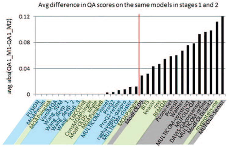
Average difference in global accuracy estimates submitted by CASP11 predictors on the same models in two different stages of the EMA experiment. Groups are sorted by the increasing average absolute difference between the stage 1 and stage 2 scores. The red vertical line (corresponding to a difference of 0.02) separates methods that generate approximately the same accuracy scores for the same models in both stages of the experiment (left) and those that do not (right). Single-model methods (blue) and clustering methods (grey) are on different sides of the line. Quasi-single methods (green) can be found on the both sides of the separation line.

$$\mathit{\text{diff}}(\mathit{\text{METHOD}})=\frac{1}{N}{\sum }_{n\in S_1\cap S_2}|{\mathit{\text{QAscore}}}_1(n)-{\mathit{\text{QAscore}}}_2(n)|,$$

where S_i is the dataset of all models (on all targets) released in the i^th stage of the experiment (i.e., S₁=sel20 and S₂=best150); QAscore_i (n) is METHOD's accuracy estimate for model n in the i^th stage; n=1,…,N – common models from S₁ and S₂ datasets. As one can see from Figure 1, the diff parameter for CASP11 methods gradually increases from 0 to 0.012, and then jumps to 0.03 at the position where the first clustering method (ModFOLD5) is found. Thus, the data provide a natural separation (shown as a vertical red line in Figure 1) between the methods generating very similar accuracy scores for the same models in both stages of the experiment and those that do not. In other words, methods on the left of the vertical line can provide accuracy estimates using a single model, while the remaining ones require a set of models as input. This diff-based separation perfectly corresponds to the methodology-based classification, with all single-model methods being to the left of the separation line and all clustering methods to the right. Quasi-single methods can be found on both sides of the separation line thus showing their different levels of dependency on the number and distribution of the models in the data set.

2. Estimation of global accuracy of models

An a-priori estimate of the global accuracy of a model can serve as a first filter in determining the usefulness of the model to address a specific problem. In this paper we assess the effectiveness of QA methods to assign overall accuracy score to a model by evaluating their ability to (1) find the best model amongst many others, (2) discriminate between good and bad models, (3) assign a correct relative score to a model (i.e., correctly rank the models) and (4) assign a correct absolute score.

2.1. Identifying the best models (QAglob.PT)

One of the most important tasks for accuracy estimation methods is identifying the best models from among several available. To assess the “best selector” performance, we calculated the difference in scores between the models predicted to be the best and the actual best models, i.e. those with the highest similarity to the native structure for each target and dataset. We used the GDT_TS, CADaa, LDDT and SG scores for this analysis (see Methods). The results showed that the correlation between the different measures can be as low as 0.61 (between the GDT_TS and CADaa on the best150 datasets), indicating that the addition of local similarity measures provides information not readily identified by the GDT_TS alone^§. As the GDT_TS score is more sensitive to the relative orientation of domains than the rigid-body superposition-free measures, it could be surmised that the difference is the result of the fact that the accuracy scores are assigned to whole targets, while the similarity of the model with the native structure is computed for each domain separately. Our analysis, though, does not support this hypothesis since the evaluations on all targets (AT) and single-domain targets only (SDT) generate very similar results by all measures, including GDT_TS (CC_{GDT_TS}[AT_vs_SDT]=0.99), and therefore the difference in the scores is apparently due to differences in the methods and not to the specific assessment procedure.

Clearly, measuring the difference in accuracy between the predicted best model and the actual best makes sense only if the best model is of good quality itself. Consequently we performed this analysis only on targets for which at least one model scored above cutoffs set to 40 for GDT_TS and SG scores, and to 0.4 for CADaa and LDDT.

2.1.1. How far away are the best EMA models from the best available?

Figure 2 illustrates the accuracy of CASP11 methods in selecting the best models according to the GDT_TS score. The figure shows that two EMA methods (Wallner and Pcons-net, both clustering-based) are capable of identifying the best models in the best150 datasets with an average error (i.e. difference between the GDT_TS of the model selected as the best and the actual best one) smaller than 5 GDT_TS units, which translates into a 7% difference on the relative scale. The best single-model method (ProQ2) is forth in the ranking, just 1.4 GDT_TS units behind the best method. Pcons-net, ModFOLD5-single and ModFOLD5 are the three methods that exhibit smaller than 3 GDT_TS unit loss in accuracy on the sel20 datasets. Results of the assessment according to other scores are provided in the Supplementary Material (Figure S1) and summarized in the ranking table (Table II). The data show that some of the groups that perform best according to the GDT_TS score are consistently in the top part of the result tables according to other scores. In particular, Table II shows that five groups, including three single-model methods (ProQ2, ProQ2-refine, Multicom-novel) are among the best 10 selectors on the best150 datasets according to all four evaluation measures. Four additional groups, including one single-model method -Multicom_cluster – are in the “top 10” according to three of the measures. The relatively good performance of single-model methods is also confirmed by the data shown in Figure 3, which summarizes the performance of all CASP11 methods in terms of the cumulative z-score on the four evaluation measures. The three single-model methods closely follow the top two clustering methods. The “top 12” list includes five single-model methods, four quasi-single methods, and three clustering methods. All these methods are ranked higher than the reference Davis-QAconsensus method, which is only 15^th on the best150 datasets. It is worth mentioning that the single-model methods would have been ranked even higher (in the top four positions of the final ranking table) if only the measures based on local similarities were used for the ranking. We attribute this result to the fact that single-model methods are usually based on geometry and energy functions that pay more attention to the local correctness of models, which is the conceptual basis of non-rigid-body based similarity measures such as LDDT (which rewards the similarity of local distances), CAD (similarity of contact areas), and SG (similarity of local substructures). This hypothesis is supported by the analysis of the EMA scores of single-model methods on models with good and bad local accuracy as judged by the Molprobity¹⁴ scores. Results in Figure S2 (Supplementary material) show that correlation between the EMA scores and Molprobity scores is practically negligible for all types of methods (the highest Pearson correlation coefficient is 0.23) on both - locally good and poor models, thus indicating no significant dependency of the EMA scores on the models' local properties. Nevertheless, comparison of mean EMA scores on both subsets of data shows that single-model methods do tend to produce somewhat higher scores on stereo-chemically accurate models (thus reasonably giving an edge to the models with better local properties), while clustering and quasi-single methods are practically insensitive to local accuracy.

Figure 2.

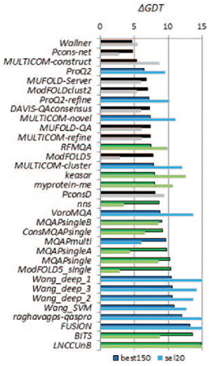
Average difference in accuracy between the models predicted to be the best and the actual best according to the GDT_TS score. For each group, the differences are averaged over all predicted targets for which at least one structural model had a GDT_TS score above 40. The graph shows the results on two datasets: best150 (upper bars, darker color) and sel20 (lower bars, lighter color). Clustering methods are in black, single-model methods in blue and quasi-single model methods in green. Groups are sorted according to the accuracy loss on the best150 datasets. Lower scores indicate better group performance. According to the global GDT_TS score alone, clustering methods occupy the top three places in the results table. The accuracy difference in identifying the best models with the best clustering method and with the best single-model method is within the 2 GDT_TS tolerance threshold used here to define similar models.

Table II.

Rankings of CASP11 QA methods based on the average loss from the best model on (A) best150 and (B) sel20 datasets according to four evaluation measures. Groups in each panel are sorted according to the increasing cumulative rank. Single-model methods are in bold, quasi-single – in italic. Results in the top ten are shaded grey.

(A, best150)					(B, sel20)
	GDT	LDDT	CAD	SG		GDT	LDDT	CAD	SG
ProQ2	4	3	4	2	Pcons-net	1	1	1	2
Wallner	1	8	1	5	nns	4	4	4	1
Pcons-net	2	11	2	3	ModFOLD5	2	12	2	3
ProQ2-refine	7	4	5	4	MQAPsingleA	5	3	5	5
MULTICOM-novel	9	1	9	7	Wallner	7	2	6	6
MULTICOM-cluster	14	2	3	8	ModFOLD5_single	3	13	3	4
MULTICOM-construct	3	10	6	9	ModFOLDclust2	6	5	7	10
RFMQA	12	5	7	6	DAVIS-QAconsensus	8	9	8	12
myprotein-me	16	6	12	1	MUFOLD-QA	11	6	11	11
nns	18	9	8	10	MUFOLD-Server	9	10	9	13
VoroMQA	19	7	11	11	ConsMQAPsingle	13	8	13	7
MUFOLD-Server	5	19	10	15	MQAPmulti	10	16	10	8
ModFOLDclust2	6	18	13	18	MULTICOM-refine	12	7	12	14
keasar	15	12	17	13	MULTICOM-construct	16	15	18	9
MUFOLD-QA	10	21	14	22	ProQ2	19	11	16	15
DAVIS-QAconsensus	8	22	15	23	MQAPsingleB	15	17	15	16
MULTICOM-refine	11	25	18	25	MQAPsingle	14	22	14	19
Wang_SVM	29	13	21	16	ProQ2-refine	21	14	17	18
PconsD	17	24	16	24	myprotein-me	22	18	19	17
Wang_deep_2	28	16	20	17	RFMQA	20	19	20	21
Wang_deep_1	26	14	22	20	BITS	17	26	21	20
Wang_deep_3	27	15	24	19	MULTICOM-novel	23	20	23	22
MQAPsingleA	23	17	25	21	PconsD	18	23	22	27
ConsMQAPsingle	21	20	32	14	MULTICOM-cluster	24	21	24	24
ModFOLD5	13	28	19	28	Wang_SVM	26	24	25	23
MQAPsingleB	20	23	33	12	VoroMQA	28	25	27	25
MQAPmulti	22	26	27	26	keasar	25	27	26	30
MQAPsingle	24	30	26	27	Wang_deep_2	27	28	28	26
ModFOLD5_single	25	32	23	30	Wang_deep_3	29	29	29	28
raghavagps-qaspro	30	27	28	29	Wang_deep_1	30	30	30	29
BITS	32	29	30	31	raghavagps-qaspro	32	31	32	31
FUSION	31	31	29	32	FUSION	31	32	31	33
LNCCUnB	33	33	31	33	LNCCUnB	33	33	33	32

Figure 3.

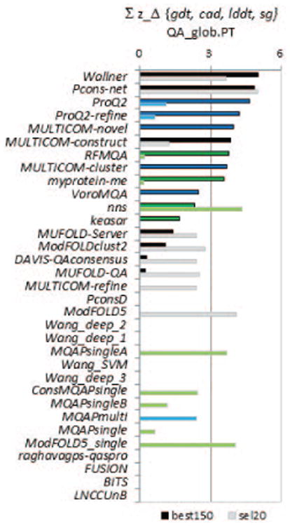
Comparison of group performance based on cumulative z-scores of the GDT_TS errors for CASP11 groups on the best150 (upper bars, darker color) and sel20 (lower bars, lighter color) datasets. The higher the score (i.e., the longer the bar), the better the group performance. Z-scores for each of the four evaluation measures (GDT_TS, LDDT, CADaa, and SG) are calculated from the distributions of the corresponding average errors and then added. Groups are sorted according to the decreasing z-scores on the best150 datasets and bars are shown only for groups with above average performance (i.e., with cumulative z_score>0). The color scheme used for the methods is the same as in Figure 2. Efficiency of the best single-model methods is comparable with that of clustering methods as three single-model methods are among the best five.

While single-model methods show a relatively good performance on the best150 datasets, quasi-single model methods show accuracy comparable to clustering methods on the sel20 datasets. Three quasi-single methods (ModFOLD5-single, nns and MQAPsingleA) together with two clustering methods (Pcons-net and ModFOLD5) appear in the “top5 lists” according to 3 out of 4 evaluation measures (Table II) and show the highest cumulative z-scores (Figure 3). Better relative performance of quasi-single methods on the sel20 datasets can be associated with the specifics of the training procedure for this type of methods, more effectively utilizing the larger spreads in model accuracy.

To establish the statistical significance of the differences in performance we performed two-tailed paired t-tests on the common sets of predicted targets and models. Table S1 in the Supplementary Material shows the results of the t-tests for each measure and each dataset separately (panels A-H), and summarizes the results for the groups appearing on the “top 15” list according to all four evaluation measures (panels I,J). The individual t-tests (panels A-H) show that, for all measures and methods, there is at least another method statistically indistinguishable from the selected method at the p=0.05 significance level, and at least five similar methods at the p=0.01 significance level. The summary table on the best150 datasets (panel I) shows that no method from the “all-measure top 15 list” can be proved significantly better than others from the same list according to the majority of the evaluation scores. As the “top performer” list includes four single-model methods alongside with three clustering methods (and one quasi-single), the tests suggest that the best performing CASP11 single-model methods perform on-par with the clustering methods in identifying the best models. On the sel20 datasets, the dominance of clustering methods is also challenged, this time by quasi-single methods, as half of the top eight significantly similar methods in panel J are quasi-single methods.

2.1.2. How often EMA methods succeed or fail in recognizing the best models?

In complement to the previous subsection and using the same evaluation data we analyze the success rate of CASP11 EMA methods in identifying the best models. We assume that a method succeeds if the difference in scores between the best EMA model and the actual best model is small (within 2 score units) and fails if the difference is bigger than 10^**. As high success rate and low failure rate are the desired features of an EMA method, we use the difference between these rates as a criterion to assess the methods' efficiency.

Figure 4 shows the percentage of targets for which the models identified as the best were 0-2, 2-10 and >10 GDT_TS units away from the actual best models. It can be seen that the top-performing EMA methods can identify the best model with an error of less than 2 GDT_TS units (green bars) for approximately one-third of the targets on the best150 sets. At the same time, these methods miss the best models by much (>10 GDT_TS units, red bars) for approximately 20% of the targets, with two methods (Pcons-net and Wallner) being an exception (failing only on 7% of the targets). Results according to other evaluation measures are shown in Figure S3 (panels A-C) of the Supplementary Material. Table III summarizes the relative performance of the groups providing ranks of their efficiency according to each of the evaluation measures. Panel A of the table confirms that single-model methods hold leading positions in the selection of the best models, with three methods of this type (Multicom-cluster, Multicom-novel and ProQ2-refine) being at the top. Similarly to the analysis in the previous section, the “top 12” list includes five single-model methods, four quasi-single methods and three clustering methods, and does not include the reference Davis-QAconsensus method.

Figure 4.

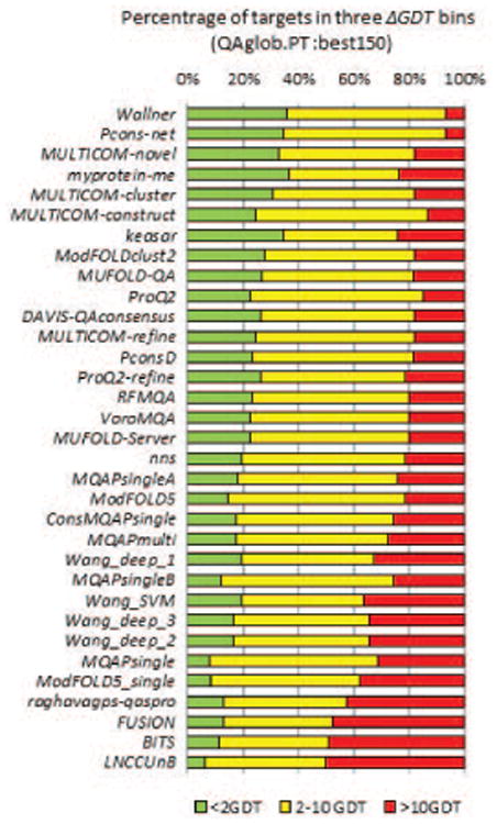
Success rates of CASP11 methods in identifying the best models. The percentage of targets where the best EMA model is less than 2 (green bars), more than 2 and less than 10 (yellow) and more than 10 (red) GDT_TS units away from the actual best model on the best150 datasets. The percentages are calculated on targets for which at least one structural model had a GDT_TS score above 40. Groups are sorted by the difference between the green and red bars. Top performing groups can correctly identify the best models in roughly one in three test cases.

Table III.

Ranking of CASP11 QA methods by the difference between the percentages of well predicted and poorly predicted targets (green bars minus red bars in Figures 4 and S2). The target is assumed to be well predicted if the best QA model is 0–2 units away from the actual best model according to the selected evaluation measure, and poorly predicted if it is more than 10 units away (LDDT and CADaa scores are preliminary multiplied by 100). The results are provided on (A) best150 and (B) sel20 datasets for four evaluation measures. Groups in each panel are sorted according to the increasing cumulative rank. Single-model methods are in bold, quasi-single – in italic. Results in the top ten are shaded grey.

(A, best150)					(B, sel20)
	GDT	LDDT	CAD	SG		GDT	LDDT	CAD	SG
MULTICOM-cluster	5	1	1	2	Pcons-net	3	1	1	1
MULTICOM-novel	3	10	2	4	Wallner	6	4	2	3
ProQ2-refine	14	4	3	1	nns	4	5	6	2
Pcons-net	2	2	11	9	MQAPsingleA	5	6	3	6
myprotein-me	4	11	4	6	ModFOLD5	2	2	15	4
Wallner	1	3	12	10	ModFOLD5_single	1	3	16	5
ProQ2	10	6	5	5	ModFOLDclust2	7	7	5	8
RFMQA	15	5	6	3	ConsMQAPsingle	9	13	4	7
MULTICOM-construct	6	9	8	13	MUFOLD-QA	12	12	7	9
keasar	7	12	10	8	MQAPmulti	8	8	11	14
VoroMQA	16	8	7	7	MUFOLD-Server	11	9	9	12
nns	18	7	9	11	DAVIS-QAconsensus	10	10	10	13
ModFOLDclust2	8	14	20	20	MULTICOM-refine	13	11	8	11
MUFOLD-Server	17	13	19	18	ProQ2	18	16	12	10
MUFOLD-QA	9	17	24	21	MQAPsingleB	14	14	17	15
DAVIS-QAconsensus	11	16	22	24	MULTICOM-construct	17	18	13	18
PconsD	13	15	23	22	ProQ2-refine	19	17	14	17
Wang_deep_1	23	25	14	15	PconsD	15	19	21	19
Wang_SVM	25	23	15	14	MQAPsingle	16	15	23	22
MQAPsingleA	19	20	17	23	myprotein-me	21	20	22	16
Wang_deep_2	27	22	16	17	MULTICOM-novel	22	21	18	21
MULTICOM-refine	12	18	29	25	RFMQA	23	22	19	20
Wang_deep_3	26	26	13	19	MULTICOM-cluster	24	24	20	25
ConsMQAPsingle	21	30	26	12	BITS	20	23	26	26
ModFOLD5	20	19	30	27	Wang_SVM	25	26	24	23
MQAPmulti	22	27	25	26	Wang_deep_2	26	25	27	27
MQAPsingleB	24	32	28	16	VoroMQA	28	28	25	24
raghavagps-qaspro	30	29	18	29	Wang_deep_3	27	27	28	28
MQAPsingle	28	24	31	28	keasar	29	29	29	29
ModFOLD5_single	29	21	33	30	Wang_deep_1	30	30	30	30
BITS	32	33	21	31	FUSION	31	31	33	32
FUSION	31	28	27	32	LNCCUnB	33	32	32	31
LNCCUnB	33	31	32	33	raghavagps-qaspro	32	33	31	33

Data for the sel20 datasets are provided in panels D-G of Figure S3 and in panel (B) of Table III. Comparing these with the best150 data, three major differences can be observed: (1) a different group of methods on the top, (2) a higher success rate of the best methods (usually above 70%), and (3) a lower failure rate (usually around 10%). The higher efficiency of the methods on the sel20 datasets is apparently related to the smaller number of models in the dataset and the larger separation in accuracy between the models.

2.1.3. Additional analysis outside of the regular CASP assessment: Identifying high accuracy outlier models

During the evaluation of model accuracy predictions it was brought to our attention by the free modeling assessor that one of the groups participating in tertiary structure prediction (G064, Baker) submitted outstanding high accuracy models for two difficult targets – T0806 and T0824. We thought it interesting to check if methods for estimation of model accuracy would be able to recognize the high level of accuracy of these models. As these models were submitted in the expert-predictor track and therefore outside of the regular server model-based assessments in the model accuracy estimation category, we asked the authors of the historically well-performing methods (Jianlin Cheng, Arne Elofsson, Liam McGuffin and Bjorn Wallner) to generate accuracy estimates for these additional models. We did not reveal the specific purpose of the request, the identity of the structure prediction group, nor the structures of the targets. Therefore, even though they were not part of the regular CASP11 EMA evaluation, the results of this exercise were generated in a blind prediction regime. Figure 5 shows that two of the single-model methods used in this exercise (ProQ2 and ProQ2-refine) were able to identify the outstanding structural models in the sets of over 450 models submitted for each of these two targets, while two other single-model methods (Multicom-cluster and Multicom-novel) succeeded on one of them (T0806). All clustering methods and a quasi-single model method from the selected research centers failed this test on both targets.

Figure 5.

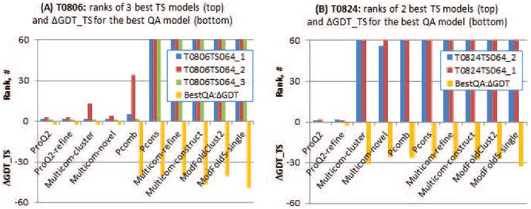
Results of ten EMA methods on two free modelling targets - T0806 (panel A) and T0824 (panel B). The top portions of the graphs show ranks of the models denoted as superior by the assessors, while the bottom portions show the difference in GDT_TS between the model with the highest predicted accuracy and the model with the highest GDT_TS score. Bars reaching the top of the scale in upper portions of the graphs indicate that the corresponding EMA methods assigned scores to the outstanding models outside the best 60. Two single-model methods, ProQ2 and ProQ2-refine, were able to correctly identify outstanding structural models among the 450 submitted on each of the targets, and assigned ranks 1 to 3 to the superior three models on T0806 and ranks 1 and 2 to the best two models on T0824.

2.1.4. Additional analysis outside of the regular CASP assessment: Model selection

We have also noticed that some well-performing groups are better than others in selecting the first model (which is expected to be the best) out of the five submitted to CASP (see Figure 6). Similar to the above (2.1.3), outside-of-the-regular-CASP analysis shows that single-model methods could have helped some of the well-performing CASP11 structure predictors in identifying their best models (Figure 7). In particular, the Baker group could have improved the accuracy of its first models by 2 GDT_TS points per target on average by using ProQ2 or ProQ2-refine method to rank the models. At the same time, using these methods for selecting Model_1 would only (slightly) worsen the results for the Zhang group, indicating that this group uses a reliable accuracy estimation method in their own structure prediction pipeline.

Figure 6.

Difference in the GDT_TS scores between the models designated as #1 and the best models (out of the five submitted) for four well performing CASP11 structure prediction groups. Each data point corresponds to one domain. Domains are sorted according to the increasing difference score for each group. Data is plotted on 78 “all-group” domains for human-expert groups (Baker and Zhang) and 126 domains for server groups. Data show that the Zhang and Zhang-server groups were able to select the best models better than the Baker and Rosetta groups. In particular, the Zhang group correctly identified the best model on 31 domains, while Baker only on 18; at the same time the Zhang group missed their best models by more than 10 GDT_TS only in 4 cases, while the Baker group in 23. The Zhang-server selected the first models within 2 GDT_TS units from the best in 82 cases (out of 126), while Rosetta for 53.

Figure 7.

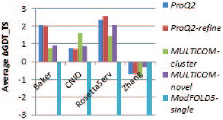
Average per-target difference in GDT_TS scores between the model with the highest accuracy score as assigned by five EMA methods and Model_1 as submitted by four structure prediction groups (x-axis of the graph). Three out of the four tested groups could have improved the accuracy of their first models using ProQ2 or ProQ2-refine method to rank their models.

2.2. Distinguishing between good and bad models (QAglob.All)

In order to assess the ability to discriminate between good and bad models, we pulled together the models for all targets (QAglob.All) and then calculated the scores on the all-model evaluation sets. This differs from the approach used in the previous section, where we first calculated scores on a per-target basis (QAglob.PT mode) and only afterwards we averaged them. The conceptual difference between these two approaches is discussed in our previous EMA evaluation paper⁶ and relates to the difference between a relative and an absolute ranking. Both analyses were performed separately on the best150 and sel20 datasets, and the area under the curve (AUC) of the Receiver Operating Characteristic (ROC) analysis was used as a measure of the methods' accuracy.^††

Figure 8 shows the ROC curves for the best 12 groups, using a threshold of GDT_TS=50 to separate good and bad models. The ROC curves according to the other evaluation measures are presented in Figure S4 of the Supplementary Material. The ROC curves for the top performing groups often look very similar, suggesting similar discriminatory power. The DeLong tests for each pair of ROC curves⁶ were performed to establish statistical significance of differences in group performance (see Table S2 in Supplementary Material). Figure 9 provides a summary in terms of the cumulative z-scores calculated on the areas under the ROC curves for the four evaluation measures.

Figure 8.

ROC curves for the best performing EMA groups according to the GDT_TS score on (A) best150 and (B) sel20 datasets. The separation threshold between good and bad models is set to GDT_TS=50. Group names are ordered according to decreasing AUC scores. The data are shown for the best 12 groups only. For clarity, only the left upper quarters of ROC curves are shown (FPR≤0.5, TPR≥0.5). Top performing groups show similar discriminatory power with clustering methods and perform slightly better than single-model methods.

Figure 9.

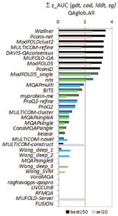
Cumulative z-scores of the AUCs for CASP11 groups on best150 (upper bars, darker colors) and sel20 (lower bars, lighter color) datasets. Z-scores for each of the four evaluation measures (GDT_TS, LDDT, CADaa and SG) are calculated from the distributions of the corresponding AUCs and then added. The higher the score, the better the group performance. Groups are sorted according to the decreasing z-scores on the best150 datasets and bars are shown only for groups with above the average performance (i.e., cumulative z_score>0). The color scheme for the methods is the same as in Figure 2. Clustering methods are shown to be superior in this analysis.

The results suggest that clustering methods are superior in this task, holding top eight positions in the ranking. This indicates that, when many models are available and need to be partitioned in two classes (good/bad), clustering methods are particularly good. Quasi-single methods can compete with clustering methods if models in the datasets are widely spread in terms of their accuracy (as in the sel20 datasets). According to the results of the DeLong statistical significance tests on the best150 datasets, the Wallner method is shown to be better than other methods (except for the statistically similar Pcons-net method) according to the majority of the measures. On the sel20 datasets this group also performs very well, while other top groups are more similar to each other.

2.3. Assigning relative model accuracy estimates (QAglob.PT & QAglob.All)

This aspect of accuracy assessment was evaluated by computing the correlation between the predicted and observed model accuracy according to the four evaluation measures.

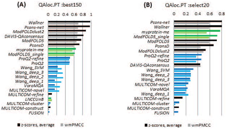
Figure 10 shows the GDT_TS-based correlation for all participating groups (A) in the per-target based mode and (B) when all models are pulled together. The best performing EMA predictors reach a wmPMCC of 0.7 on the best150 datasets and 0.9 on the sel20 datasets in the per-target assessment mode, and a PMCC of around 0.9 on both datasets in the “all models pulled together” mode. Results according to other evaluation measures (see Figure S5 of the Supplementary Material) show approximately the same values of the correlation coefficients for the top groups according to these measures. This similarity indicates that, independently of the reference measure, EMA methods are usually quite reliable (correlation coefficient above 0.8) in ranking models in diverse datasets (such as QAglob.PT:sel20, QAglob.All:best150 or QAglob.All:sel20), and somewhat less reliable when the provided models span a narrower range of accuracy (as in QAglob.PT:best150). The magnitude of the drop in the correlation scores in the second case depends on the level of similarity inside the model dataset – see our paper³. As in CASP10, the top performing EMA methods are consensus-based, with Wallner and Pcons-net leading the rankings according to the majority of scores on the best150 datasets. The dominant position of these methods is confirmed by the data in Figure 11, which shows the cumulative z-scores over four evaluation measures, and in Table S3 (Supplementary Material) where we list the results of the statistical tests on the correlation coefficients. Figure 11 also demonstrates that two single-model methods (Multicom-novel and VoroMQA) exhibit good overall correlation on the best150 datasets, mostly because they achieve high scores according to the CADaa measure (see also Figure S5(C) and Table S3(C)). This perhaps is not surprising for VoroMQA, as this method is based on the same principle as the CADaa measure (similarity of contact areas).

Figure 10.

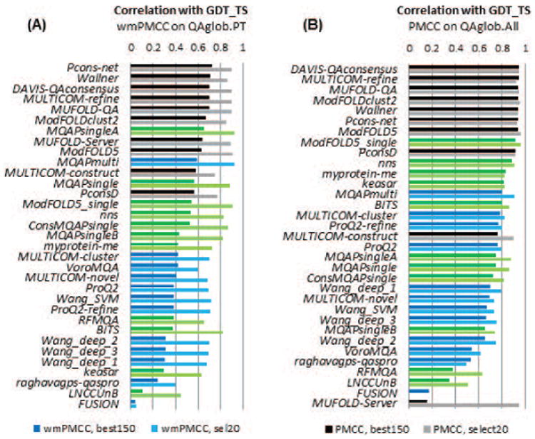
(A) Weighted means of per-target Pearson correlation coefficients (wmPMCC) and (B) Pearson correlation coefficients (PMCC) computed on the datasets comprising all models in the best150 and sel20 datasets. Each panel shows the data for two datasets: best150 (darker colors) and sel20 (lighter colors). Groups are sorted according to the decreasing correlation on the best150 datasets. The color scheme for the methods is the same as in Figure 2. The best performing methods are well equipped to correctly rank models in the datasets, showing high correlation between the predicted and actual model accuracy scores.

Figure 11.

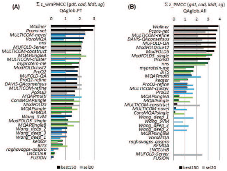
Cumulative z-scores of the correlation coefficients for CASP11 groups on best150 (upper bars, darker colors) and sel20 (lower bars, lighter colors) datasets. Z-scores for each of the four evaluation measures (GDT_TS, LDDT, CADaa and SG) were calculated from the distributions of the corresponding correlation coefficients and then summed up. The higher the score, the better the group performance. Groups are sorted according to the decreasing z-scores on the best150 datasets and bars are shown only for the groups with above the average performance (i.e., cumulative z_score>0). The color scheme for the methods is the same as in Figure 2. Two clustering methods (Wallner and Pcon-net) are apparent leaders in ranking the models. Two single-model methods (Multicom-novel and VoroMQA) hold positions 3 and 4 in ranking due to their relatively high scores on one of the local evaluation measures (CADaa).

2.4. Assigning absolute model accuracy estimates (QAglob.All)

Assigning of the model global accuracy scores was evaluated by computing the average differences between the predicted and observed model accuracies according to the four evaluation measures. These scores were calculated for all models evaluated in best150 and sel20 datasets and then averaged separately for each dataset.

Figure 12A shows the average deviation between the predicted scores and the GDT_TS score for each participating group (only positive scores are shown). The best performing EMAs predict GDT_TS score of models with an average error of 6 GDT_TS units on both datasets. Similarly to the results in relative performance analysis (2.3), all top-performing EMAs are consensus-based, with MUFOLD-QA, DAVIS-QAconsensus and MULTICOM_refine holding the lead. The best performing non-clustering methods are ModFOLD5_single and MQAPmulti, with an average error of 11 GDT_TS units. Results according to other evaluation measures are presented in Figure S6 of the Supplementary Material and summarized as z-scores in Figure 12B. The picture on the best150 datasets is clear – the top seven positions in the rankings are occupied by clustering methods and they are well separated from the following two single-model methods in terms of performance.

Figure 12.

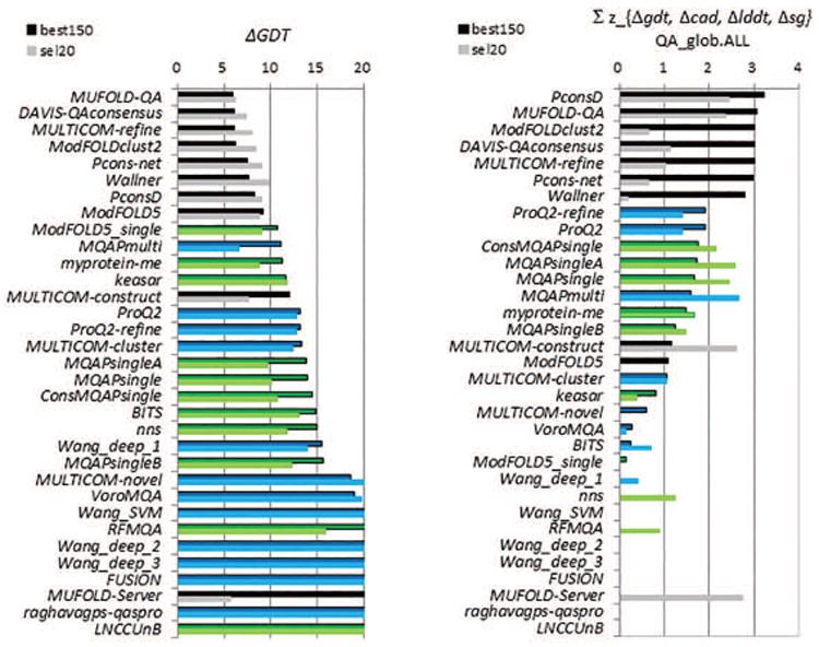
(A) Average deviations of accuracy estimates from GDT_TS scores of the assessed models. For each group, the deviations are calculated for each model and then averaged over all predicted models. Lower scores indicate better group performance. (B) Cumulative z-scores of the deviations of absolute accuracy estimates for the CASP11 groups. Z-scores for each of the four evaluation measures (GDT_TS, LDDT, CADaa, and SG) are calculated from the distributions of the corresponding average errors and then added. The higher the score, the better the group performance. Data bars are shown only for groups with above the average performance. In both panels, graphs show the results for two datasets: best150 (upper bars, darker color) and sel20 (lower bars, lighter color). Clustering methods are in black, single-model methods in blue and quasi-single model methods in green. Groups are sorted according to the results on the best150 datasets. The best performing methods are capable of predicting the absolute accuracy of models with an average per-target error of 6 GDT_TS.

3. Estimation of local accuracy of models

While the global model accuracy scores provide estimates of overall model quality, per-residue scores offer estimates of the correctness of the local structure and geometry. The local accuracy estimates can help recognize the well-modeled regions in relatively bad models and, vice versa, poorly modeled regions in overall good models. Here we assess the effectiveness of local estimators by verifying how well these methods (1) assign correct distance errors at the residue level, and (2) discriminate between reliable and unreliable regions in a model.

3.1. Assigning proper error estimates to the modeled residues (QAloc.PT)

For the twenty-one groups that submitted model confidence estimates at the level of individual residues, we measured the correlation between predicted and observed distance errors, setting all values exceeding 5Što 5ų.

Panels A and B in Figure 13 show the mean z-scores and weighted means for PMCCs for the participating groups on the best150 and sel20 model sets, respectively. As in CASP10, two clustering methods (Pcons-net and Wallner) achieve the highest scores on both datasets. On the best150 datasets, these groups are significantly better than all the others; on the sel20 datasets they are statistically indistinguishable from each other and from two other groups -ModFOLD5 and ModFOLD5_single, and better than the remaining groups (see Table S4, Supplementary Material). Two quasi-single methods (myprotein-me and ModFOLD5_single) reach correlation coefficients around 0.6 on both datasets, a figure just slightly smaller than that for the best pure clustering methods.

Figure 13.

Correlation analysis for 20 individual groups and the Davis-QAconsensus reference method for the per-residue accuracy prediction category. Correlation analysis results are calculated on a per-model basis and subsequently averaged over all models and all targets in the (A) best150 and (B) sel20 datasets. The color scheme for the methods is the same as in Figure 2. The best methods show a correlation of just above 0.6 in local accuracy estimates.

3.2. Discriminating between good and bad regions in the model (QAloc.All)

To evaluate the accuracy with which the correctly predicted regions can be identified, we pulled the submitted estimates for all residues from all models and all targets (over 3,300,000 residues from over 13,000 models per EMA predictor in the best150 datasets and approximately 440,000 residues from over 1,700 models in the sel20 sets). We calculated the Matthews correlation coefficient for these residues and carried out the ROC analysis (see our CASP10 assessment paper⁶ for details). Similarly to global classifiers (i.e., good/bad models), the ranking of local classifiers (reliable/unreliable residues) appears to be very similar according to the Matthews correlation coefficient and the ROC analysis, therefore we only discuss here the results of the ROC analysis.

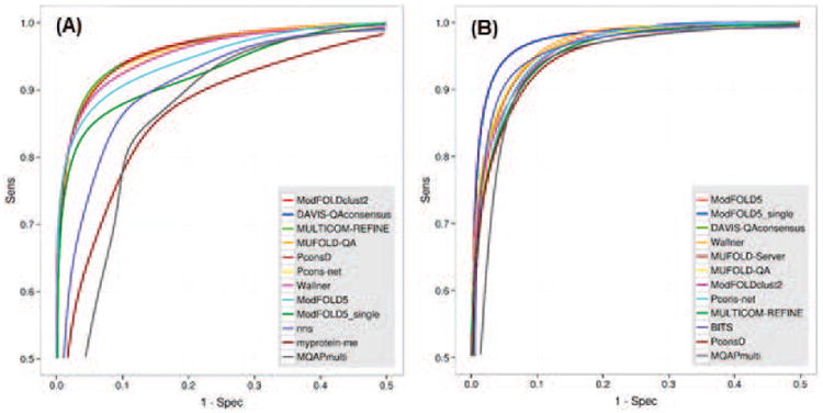
Figure 14 demonstrates that, similarly to CASP10, two methods from the L. McGuffin group (University of Reading, UK), namely ModFOLDclust2 and ModFOLD5, are on top of the list of the local classifiers. In general, the difference between the best predictors in terms of the AUC is very small as the AUC bars in the insets of Figure 14 are practically of equal height for the first five groups on the best150 datasets and for the first four groups on the sel20 datasets. The reference DAVIS-QAconsensus method is among the best methods on both datasets, indicating that no method can significantly outperform the simple clustering approach. The best quasi-single method (ModFOLD5_single) just slightly lags behind the top 5 methods on the best150 datasets and is the third on the sel20 datasets, which is a reasonably good result. Single-model methods are in the bottom part of the result tables according to both evaluation procedures (i.e., 3.1 and 3.2) of the QAloc analysis.

Figure 14.

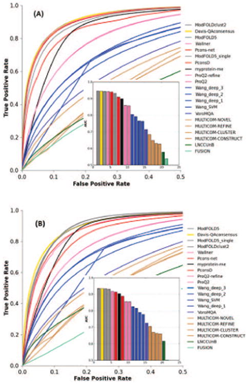
Accuracy of the binary classifications of residues (reliable/unreliable) based on the results of the ROC analysis for (A) best150 and (B) sel20 datasets. A residue in a model is defined to be correct when its Cα is within 3.8Å from the corresponding residue in the target. For clarity, only the left half of a typical ROC-plot is shown (FPR≤0.5). Group names are ordered according to decreasing AUC scores; the inset shows the AUC38 scores for the corresponding ROC curves. (AUC38 = AUC with the 3.8Å cutoff). The ModFOLDclust2 and ModFOLD5 methods are on top of the list of the local classifiers; the reference Davis_QAconsensus method shows comparable results.

4. Ability to self-assess the reliability of model coordinates in TS modeling (QAself)

Providing realistic error estimates for residues in structural models increases the usefulness of structure prediction methods and is an essential guide for real-life applications.

To evaluate the ability of TS predictors to assign realistic error estimates to the coordinates of their own models, we computed the log-linear Pearson correlation between the observed and predicted residue errors and performed a ROC analysis. The assessment was performed separately for all participating groups on a subset of “all-group” targets (Figure 15), and for server predictors on all targets (Figure S7 in Supplementary Material). Two groups (Pcons-net and IntFOLD3, both servers) lead all ranking lists in the QAself category. They show correlation coefficients above 0.6 on a subset of “all-group” targets, and of around 0.75 on all assessed targets. Their AUCs are above 0.8 on “all-group” targets and at the 0.9 level for all targets (ROC curves themselves are shown in Figure S8). These two groups are statistically indistinguishable from each other according to the results of the DeLong and z-tests with 0.05 significance level, and better than all other QAself estimators, except for one correlation-based similarity case (see Table S5 in Supplementary Material). As the QAloc and QAself categories are conceptually similar, it is not surprising that the best-performing predictors in these two categories were developed by the same research groups (led by A. Elofsson and L. McGuffin).

Figure 15.

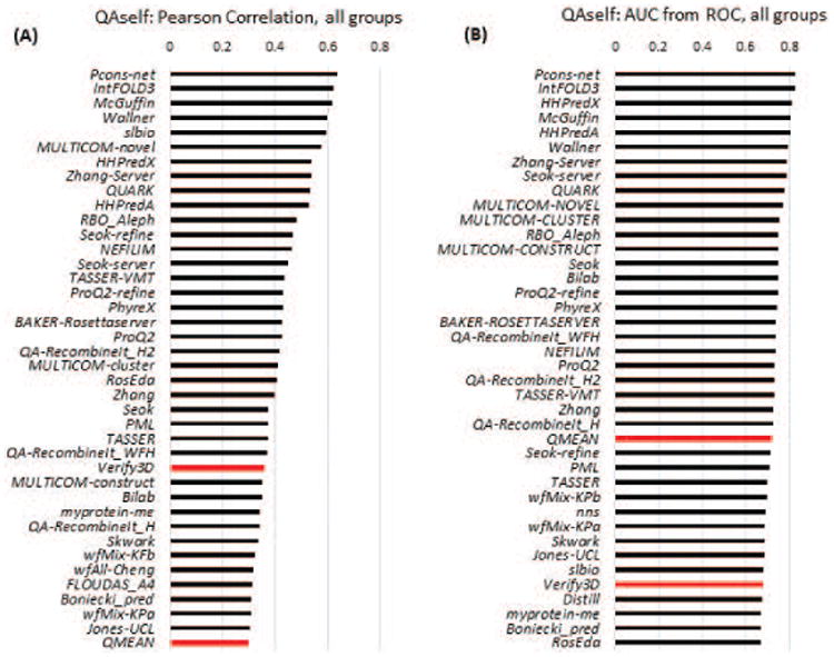
Assessment of per-residue confidence estimates (QAself) on “all-group” targets. Data are provided for the top 38 groups and two baseline single-model EMA methods - Verify3D and QMEAN (red bars). (A) Log-linear Pearson correlation coefficients. (B) AUC values from the ROC curve analysis with the cutoff of 3.8 Å separating correctly/incorrectly modeled residues.

In order to provide a baseline estimate of the accuracy of the QAself predictions, we compared them with the per residue accuracy estimates from two single-model EMA methods not participating in CASP: QMEAN¹⁵ and Verify3D¹⁶. Figures 15 and S6, and Table S5 demonstrate that the top ranked CASP11 methods perform better than these baseline methods.

Figure 16 (panels A and B) visualizes the striking difference, in terms of PMCC, between the local error estimates provided by one of the leading QAself groups, Pcons-net (TS410), and the group LEER (TS044), which ranks among the best in the TBM category. One can easily notice the good correlation between the observed and predicted error values for the first group, and essentially no correlation for the second. We believe that assigning confidence estimates to the coordinates should be common practice for structure predictors, and strongly encourage predictors to provide such estimates.

Figure 16.

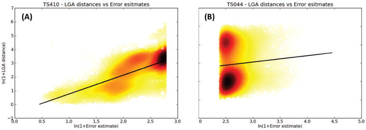
Predicted residue errors vs. observed distances for two CASP11 groups: (A) TS410 (Pcons-net) and (B) TS044 (LEER). The straight black lines represent the least-squares fitted curves described by first-degree polynomials.

To conclude this section we want to mention that not all the values provided in the B-factor field of the models could be sensibly interpreted as distances. In particular, 49 out of 96 groups submitted values higher than 99 at least once, and 44 groups submitted values averaging 20 or higher (see Table S6). As these numbers are too high to be considered reasonable distance estimates, some groups have either misinterpreted the format or perhaps attempted predicting crystallographic B-factors rather than position errors.

To give these groups the benefit of doubt and to attempt a correct interpretation of the submitted values, we calculated the RMSD between the predicted errors and (1) the actual Cα -Cα distances d between the corresponding atoms in the optimal model-target LGA superposition, and (2) pseudo B-factors derived from these distances using the formula B = 8π² d²/3 ¹⁷. Only six predictors (TS193, TS212, TS171, TS452, TS335, TS414 – see CASP11 web site for the group names) submitted confidence estimates that are more similar to crystallographic B-factors than distances (green-shaded cells in Table S6). For these six groups this analysis nevertheless showed that even with the benefit of doubt they would not be among the best performers.

5. Progress and comparison with the reference methods

Estimation of the CASP-to-CASP progress is always somewhat tricky as it is difficult to disentangle the effect of methodological advances from the differences in target difficulty and assessment procedures, or the evolution of databases. The CASP11 vs. CASP10 comparison is not an exception since the target sets appear to be of identifiably different predictive difficulty (see Figure 17); the databases grew; the experiment conditions changed (different number of servers resulted in different percentage of models included in the QA datasets, thus affecting the overall model quality spread); and the assessment procedures evolved.

Figure 17.

(A) Average minimum (lower margin of the bar), average mean (black line in the middle of the bar) and average maximum GDT_TS score (upper margin of the bar) for the models included in the best150 and sel20 datasets. CASP11 bars are in green, CASP10 in blue. The data for the best150/sel20 sets are shown in the left/right half of the graph in darker/lighter colors, respectively. It can be seen that structural models in the CASP11 QA datasets have, on average, lower accuracy and larger spread than those in the corresponding CASP10 sets. (B,C) Range of GDT_TS scores for models in CASP11 and CASP10 sel20 datasets. Each bar corresponds to one target. Targets are sorted by increasing maximum GDT_TS. It can be seen that the sel20 datasets contained inaccurate models for all targets in CASP11 (resulting in a low average mean around 10 – see panel A), and only for some in CASP10 (average mean around 30).

To provide a baseline for QAglob and QAloc methods' performance, we used the in-house developed DAVIS-QAconsensus method that has not changed since its first implementation in CASP9. Ratio between the scores of this method in different rounds of CASP may serve as an estimate of the expected change in performance due to non-methodological factors. If this change is small compared with the results of the best methods (i.e., if the CASP-to-CASP ratio of scores of the best methods exceeds that of the reference method), it may indicate progress in the field. In QAself, we used single-model EMA methods QMEAN and Verify3D as baseline methods.

5.1. Progress in estimation of overall model accuracy (QAglob)

Figure 18 shows the results of the comparison of the best methods and the reference DAVIS-QAconsensus method in CASP11 and CASP10 in the QAglob (first five scores along the x-axis) and QAloc (last two scores) analyses. The best150 datasets in CASP11 were more challenging than those in CASP10 for identifying best models as scores of the reference method (blue bars) dropped by more than 30% in both components of this analysis (Loss, 2.1.1 and Efficiency, 2.1.2). At the same time, these datasets appeared approximately of the same difficulty for good/bad model separation task (AUC, 2.2) and all-model correlation analysis (PMCC, 2.3), and easier for the per-target correlation analysis (wmPMCC, 2.3). Results of the best methods (red bars) remained practically unchanged for the “loss” and improved by 15% for the “efficiency”, thus suggesting relative progress according to both measures. There was no improvement in performance according to the AUC and PMCC analyses (bars very close to 1.0 and very similar to the reference method). Per-target correlation (wmPMCC) of the best methods improved by 18% (from 0.62 to 0.73 – absolute data are not shown on the graph), but the correlation for the reference method also grew by the same amount, thus suggesting that the increase in the correlation scores can be associated with the difference in the composition of the model datasets rather than with advancements in methodology. Data in panel (B) suggest conceptually similar conclusions on the progress of methods on the sel20 datasets, with the largest improvements in the loss-based analysis (average loss decreased by 27% from 3.40 to 2.67) and efficiency (increased by 39% from 0.52 to 0.73). Again, we underscore that these data should be taken with a grain of salt as the composition of sel20 datasets is very different in CASP10 and CASP11 (compare panels B and C in Fig.17).

Figure 18.

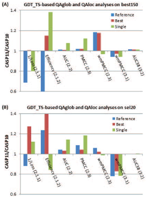
CASP11/CASP10 ratio in scores for the reference DAVIS-QAconsensus method and the best QAglob and QAloc methods in the GDT_TS-based evaluations on (A) best150 and (B) sel20 datasets. The first five scores along the x-axis are for the QAglob analysis (sections 2.1-2.3 in the text), the last two – for the QAloc (sections 3.1.-3.2). The ratio for the loss (2.1.1) is calculated on the inversed scores since in this case a lower value corresponds to better performance; the efficiency of recognizing the best models is evaluated in terms of the difference between the success and failure rates (see section 2.1.2). Values above 1.0 indicate better results in CASP11 than in CASP10. Cases where the ratios for the best methods are higher than those for the reference method may indicate methodological improvements.

Relative increase in scores for the best single model methods was higher than that for the reference method in four out of five components of the QAglob analysis (except for wmPMCC) on the best150 datasets, and in three out of five components (except for wmPMCC and efficiency) on the sel20 datasets, which can be indicative of the progress in the development of this type of methods.

5.2. Progress (or lack thereof) in estimation of local model accuracy (QAloc)

The data for QAloc show that the correlation on the per-residue distances (wmPMCC, 3.1) dropped in CASP11 for all types of methods on both datasets (red and green bars in the second to last column in Figure 18 are below the 1.0 line). As correlation for the reference method also dropped by approximately the same rate (blue bars), this suggests a “no change” conclusion. The same conclusion can be drawn from the analysis of the ability to differentiate between the reliable and unreliable regions in models (AUC38, 3.2) as the results for the reference method and the best methods did not change much since CASP10.

5.3. Progress in estimation of errors in own structural models (QAself)

In general, more predictors submitted reasonable per-residue error estimates for their models in CASP11 than in CASP10. Figure 19 shows that more ROC curves in CASP11 run closer to the left upper corner of the plot, indicating more successful predictors (i.e. those with low false positive rate and high true positive rate). The data also shows that many more methods in CASP11 are doing better than the baseline method: while in CASP10 the QMEAN method was #7 on the human/server targets, and #3 on all targets (according to the AUC), in CASP11 it was correspondingly #23 and #12 (see Figures 15 and S6). The median correlation coefficient between the actual and estimated distances rose from around 0.10 in the two previous CASPs to 0.25 in CASP11, supporting the ROC-based conclusion.

Figure 19.

Comparison of the ROC curves for QAself predictors in (A) CASP11 and (B) CASP10. In CASP10, there were only 6 groups from 2 research centers (L.McGuffin and A.Elofsson) with reasonably predicted distance errors. A big gap between ROC curves for these 6 top methods and the remaining ones is noticeable. In CASP11 there are many more predictors generating reasonable distance error scores than in previous experiments.

Figure 20 shows the results of the comparison of the best methods and the reference method (QMEAN) in CASP11 and CASP10 for the QAself estimates. It can be seen that red bars dropped slightly below the 1.0 line in all four cases, indicating the decreasing evaluation scores. In particular, the correlation scores (PMCC, 4.1) dropped for the best groups on a subset of “all-group” targets by 9% (from 0.70 to 0.64) and for server groups on all targets by 3% (from 0.78 to 0.76). As the scores for the reference method decreased much more (31% for all groups (0.44 to 0.30) and 23% for servers (0.52 to 0.40)), we can conclude that the drop in the correlation for the best CASP methods is more than offset by the change in targets' difficulty for this type of the analysis.

Figure 20.

CASP11/CASP10 ratio in scores for the reference QMEAN method and the best QAself methods for (A) all groups on “all-group” targets and (B) server groups on all CASP11 targets. Values above 1.0 indicate better results in CASP11 than in CASP10. Cases where ratios for the best methods are higher than those for the reference method may indicate methodological improvements.

Conclusions

The detailed analysis presented here will hopefully be valuable for developers of the methods for estimation of model accuracy to understand the bottlenecks to progress and where they should focus their future efforts, but it also contains useful suggestions for other scientists, users and developers of structure prediction methods in general. In the following, we summarize conclusions and some rules of thumb that should be taken into account when selecting the appropriate method to use.

1. When models from more than one structure prediction server are available or when a server produces a list of models and the task is to choose the most plausible ones, a user can take advantage of either single-model or clustering EMA methods since they are equally effective in identifying the best models. The expected selection error for the best methods is around 7% in terms of the GDT_TS score. The most successful single-model method available as a public server is ProQ2.

2. If a user wishes to filter out “worse” models from a set, the suggestion deriving from this analysis is to take advantage of clustering methods. The same is true if a ranked list of the models is needed. Pcons-net and Wallner methods consistently appear among the leading groups across the board of assessment modes and evaluation scores.

3. If a user has a single model, clustering EMA methods are not applicable. To estimate the overall correctness of the model's backbone, the best choice would be the quasi-single method ModFOLD5_single. The expected estimate error, though, is quite high, at 11 GDT_TS units. If a user is interested not only in the overall fold accuracy, but also in local features of the model (e.g., correctness of reproducing contacts), methods from the ProQ2 and MQAP series would be the best bet.

4. Accuracy at the level of individual residues is usually better predicted by clustering methods, including methods from the Pcons and ModFold family. Nevertheless, quasi-single methods, such as myprotein-me and ModFOLD5_single show accuracy just slightly lower than that of the best pure clustering methods. These methods can be helpful for assigning residue reliability scores for models selected as candidates for molecular replacement experiments in X-ray crystallography.

5. More structure predictors (15 in CASP11 vs 6 in CASP10) put effort in assigning local error estimates to their models. This speaks well about the development of the field. We expect that more and more often users will receive models annotated with expected accuracy. We prompt the users to take advantage of this information when it is available. In CASP11, the Pcons-net and IntFOLD3 methods showed the best performance in this category according to all evaluation scores.

6. It is important to notice that scores for the best global and local accuracy prediction methods did (slightly) improve in CASP11 compared to CASP10. We showed that this is not necessarily due to methodological improvements, but to other factors. On one side, this is not very satisfactory and should prompt predictors to explore other avenues. On the other, users can expect that the predictions they obtain will continue to improve as, for example, the size of databases increases.

In summary, we hope that the results of the thorough analysis of the results of this large world-wide experiment will be instrumental to direct the future development of the field and be informative for model users. In particular, we would like to stress that the observed progress in selecting the best model from a set is welcome and interesting, but should also be complemented by more efforts in annotating quality at the residue level. Some progress has been observed in this area, but perhaps some pressure from the users in requiring that a model is regularly provided together with an accuracy estimate might also help pushing the field in the right direction.

Supplementary Material

Supp TableS1-S6 & FigureS1-S8

Figure S1. Average difference in accuracy between models predicted to be the best and the actual best according to the (A) LDTT, (B) CADaa and (C) SG scores. For each group, the differences are averaged over all predicted targets for which at least one structural model had a score above 40 (LDDT and CADaa scores multiplied by 100). The graph shows results for two datasets: best150 (upper bars, darker colors) and sel20 (lower bars, lighter colors). Clustering methods are in black, single-model methods in blue, and quasi-single model methods in green. Groups are sorted according to the increasing accuracy loss on the best150 datasets. Lower scores indicate better group performance.

Figure S2. Comparison of the EMA scores for single, clustering and quasi-single methods on models with the relatively good and the relatively bad stereo-chemical characteristics. (A, B)- analysis on models with inaccurate coordinates (GDT_TS<50); (C, D)- analysis on models with quite accurate coordinates (GDT_TS≥50). (A, C) Pearson correlation coefficients between EMA scores and Molprobity scores for models of good and poor stereo-chemistry (i.e., models with the bottom 20% and top 20% Molprobity scores, correspondingly). The correlation was computed for the sets of five diverse better-performing methods in each of the categories: single-model methods (ProQ2, ProQ2-refine, Multicom-cluster, Multicom-novel, VoroMQA), quasi-single methods (ModFOLD5_single, MQAP_singleA, myprotein-me, RFMQA, Keasar) and clustering methods (Wallner, Pcons-net, ModFOLD5, ModFOLDclust2, Multicom-refine). The results show that the correlation is practically negligent for all types of methods on both - locally good and poor models, thus indicating no significant dependency of the EMA scores on models' local properties. (B, D) Mean EMA scores for single-model, clustering and quasi-single methods computed on models of good and poor stereo-chemistry separately. Single-model methods do tend to produce noticeably higher scores (though not significantly higher) on stereo-chemically accurate models thus reasonably giving an edge to the models with better local properties, while clustering and quasi-single methods are less sensitive to local accuracy.

Figure S3. The percentage of targets where the best EMA model is less than 2 (green bars), more than 2 and less than 10 (yellow) and more than 10 units away from the actual best model on the best150 datasets according to the (A) LDTT, (B) CADaa and (C) SG scores. The percentages are calculated on targets for which at least one structural model had a GDT_TS score above 40 (LDDT and CADaa scores are multiplied by 100). Groups are sorted by the difference between the green and red bars.

Figure S4. ROC curves for the best performing EMA groups according to the LDTT (panels A,B), CADaa (panels C,D) and SG scores (panels E,F) on the best150 and sel20 datasets. The separation threshold between good and bad models is set to 0.5 (50 for SG). Group names are ordered according to decreasing AUC scores. The data are shown for the best 12 groups only. For clarity, only the left upper quarters of ROC curves are shown (FPR≤0.5, TPR≥0.5).

Figure S5. Correlation coefficients for the 32 participating groups and the reference Davis-QAconsensus benchmarking method according to LDTT (panels A,B), CADaa (panels C,D) and SG scores (panels E,F) on the best150 and sel20 datasets. Each panel shows the data for two datasets: best150 (darker colors) and sel20 (lighter colors). Groups are sorted according to the decreasing correlation on the best150 datasets. The color scheme for the methods is the same as in Figure 2.

Figure S6. Average deviations of model accuracy estimates from (A) LDTT, (B) CADaa and (C) SG scores of the models. For each group, the deviations are calculated for each model and then averaged over all predicted models. The graph shows results for two datasets: best150 (upper bars, darker colors) and sel20 (lower bars, lighter colors). Clustering methods are in black, single-model methods in blue, and quasi-single model methods in green. Groups are sorted according to the increasing accuracy loss on the best150 datasets. Lower scores indicate better group performance.

Figure S7. Assessment of per-residue confidence estimates (QAself) for server groups. Data are provided for the top 38 groups and two baseline single-model EMA methods - Verify3D and QMEAN (red bars). (A) Log-linear Pearson correlation coefficients. (B) AUC values from the ROC curve analysis with the cutoff of 3.8 Å separating correctly/incorrectly modeled residues.

Figure S8. ROC curves for the participating CASP11 methods and two baseline single-model EMA methods – Verify3D and QMEAN. (A) All groups on “all-group” targets. (B) Server groups on all targets. The data for the two baseline methods are plotted as thicker black lines; the Verify3D curve is dashed. The lines in color refer to the methods that performed better than the QMEAN (in terms of AUC); the grey lines refer to those that performed worse. Methods from the same research center are plotted in the same color.

Abbreviations

EMA

Estimation of Model Accuracy

MQA

Model Quality Assessment

QAglob.PT

per-target global quality assessment

QAglob. All

all models pooled together global quality assessment

QAloc.PT

per-target local quality assessment

QAloc.All

all models pooled together local quality assessment

QAself

self-assessment of residue error estimates

best150

a dataset comprised of the best 150 models submitted on a target according to the benchmark consensus method

sel20

a dataset comprised of 20 models spanning the whole range of server model difficulty on each target

TS

Tertiary Structure

ROC

Receiver Operating Characteristic

GDT_TS

Global Distant Test – Total Score

CC

Correlation Coefficient

PMCC

Pearson's product-Moment Correlation Coefficient

MCC

Matthews' Correlation Coefficient

wmPMCC

weighted mean of PMCC

References

- 1.Schwede T, Sali A, Honig B, Levitt M, Berman HM, Jones D, Brenner SE, Burley SK, Das R, Dokholyan NV, Dunbrack RL, Jr, Fidelis K, Fiser A, Godzik A, Huang YJ, Humblet C, Jacobson MP, Joachimiak A, Krystek SR, Jr, Kortemme T, Kryshtafovych A, Montelione GT, Moult J, Murray D, Sanchez D, Sosnick TR, Standley DM, Stouch T, Vajda S, Vasquez M, Westbrook JD, Wilson IA. Outcome of a workshop on applications of protein models in biomedical research. Structure. 2009;17(2):151–159. doi: 10.1016/j.str.2008.12.014. [DOI] [PMC free article] [PubMed] [Google Scholar]
- 2.Kryshtafovych A, Fidelis K. Protein structure prediction and model quality assessment. Drug Discov Today. 2009;14(7/8):386–393. doi: 10.1016/j.drudis.2008.11.010. [DOI] [PMC free article] [PubMed] [Google Scholar]
- 3.Kryshtafovych A, Fidelis K, Tramontano A. Evaluation of model quality predictions in CASP9. Proteins. 2011;79(Suppl 10):91–106. doi: 10.1002/prot.23180. [DOI] [PMC free article] [PubMed] [Google Scholar]
- 4.Cozzetto D, Kryshtafovych A, Ceriani M, Tramontano A. Assessment of predictions in the model quality assessment category. Proteins. 2007;69(Suppl 8):175–183. doi: 10.1002/prot.21669. [DOI] [PubMed] [Google Scholar]
- 5.Cozzetto D, Kryshtafovych A, Tramontano A. Evaluation of CASP8 model quality predictions. Proteins. 2009;77(Suppl 9):157–166. doi: 10.1002/prot.22534. [DOI] [PubMed] [Google Scholar]
- 6.Kryshtafovych A, Barbato A, Fidelis K, Monastyrskyy B, Schwede T, Tramontano A. Assessment of the assessment: Evaluation of the model quality estimates in CASP10. Proteins. 2014;82(Suppl 2):112–126. doi: 10.1002/prot.24347. [DOI] [PMC free article] [PubMed] [Google Scholar]
- 7.Zemla A. LGA: A method for finding 3D similarities in protein structures. Nucleic Acids Res. 2003;31(13):3370–3374. doi: 10.1093/nar/gkg571. [DOI] [PMC free article] [PubMed] [Google Scholar]
- 8.Mariani V, Biasini M, Barbato A, Schwede T. lDDT: a local superposition-free score for comparing protein structures and models using distance difference tests. Bioinformatics. 2013;29(21):2722–2728. doi: 10.1093/bioinformatics/btt473. [DOI] [PMC free article] [PubMed] [Google Scholar]
- 9.Olechnovic K, Kulberkyte E, Venclovas C. CAD-score: a new contact area difference-based function for evaluation of protein structural models. Proteins. 2013;81(1):149–162. doi: 10.1002/prot.24172. [DOI] [PubMed] [Google Scholar]
- 10.Kryshtafovych A, Monastyrskyy B, Fidelis K. CASP prediction center infrastructure and evaluation measures in CASP10 and CASP ROLL. Proteins. 2014;82(Suppl 2):7–13. doi: 10.1002/prot.24399. [DOI] [PMC free article] [PubMed] [Google Scholar]
- 11.McGuffin LJ, Buenavista MT, Roche DB. The ModFOLD4 server for the quality assessment of 3D protein models. Nucleic Acids Res. 2013;41(Web Server issue):W368–372. doi: 10.1093/nar/gkt294. [DOI] [PMC free article] [PubMed] [Google Scholar]
- 12.Skwark MJ, Elofsson A. PconsD: ultra rapid, accurate model quality assessment for protein structure prediction. Bioinformatics. 2013;29(14):1817–1818. doi: 10.1093/bioinformatics/btt272. [DOI] [PubMed] [Google Scholar]
- 13.Ray A, Lindahl E, Wallner B. Improved model quality assessment using ProQ2. BMC Bioinformatics. 2012;13:224. doi: 10.1186/1471-2105-13-224. [DOI] [PMC free article] [PubMed] [Google Scholar]
- 14.Chen VB, Arendall WB, 3rd, Headd JJ, Keedy DA, Immormino RM, Kapral GJ, Murray LW, Richardson JS, Richardson DC. MolProbity: all-atom structure validation for macromolecular crystallography. Acta Crystallogr D Biol Crystallogr. 2010;66(Pt 1):12–21. doi: 10.1107/S0907444909042073. [DOI] [PMC free article] [PubMed] [Google Scholar]
- 15.Benkert P, Kunzli M, Schwede T. QMEAN server for protein model quality estimation. Nucleic Acids Res. 2009;37(Web Server issue):W510–514. doi: 10.1093/nar/gkp322. [DOI] [PMC free article] [PubMed] [Google Scholar]
- 16.Eisenberg D, Luthy R, Bowie JU. VERIFY3D: assessment of protein models with three-dimensional profiles. Methods Enzymol. 1997;277:396–404. doi: 10.1016/s0076-6879(97)77022-8. [DOI] [PubMed] [Google Scholar]
- 17.Wilmanns M, Nilges M. Molecular replacement with NMR models using distance-derived pseudo B factors. Acta Crystallogr D Biol Crystallogr. 1996;52(Pt 5):973–982. doi: 10.1107/S0907444996003393. [DOI] [PubMed] [Google Scholar]
Associated Data
This section collects any data citations, data availability statements, or supplementary materials included in this article.
Supplementary Materials