Hierarchical Distributed-Lag Models: Exploring Varying Geographic Scale and Magnitude in Associations Between the Built Environment and Health

Abstract

It is well known that associations between features of the built environment and health depend on the geographic scale used to construct environmental attributes. In the built environment literature, it has long been argued that geographic scales may vary across study locations. However, this hypothesized variation has not been systematically examined due to a lack of available statistical methods. We propose a hierarchical distributed-lag model (HDLM) for estimating the underlying overall shape of food environment–health associations as a function of distance from locations of interest. This method enables indirect assessment of relevant geographic scales and captures area-level heterogeneity in the magnitudes of associations, along with relevant distances within areas. The proposed model was used to systematically examine area-level variation in the association between availability of convenience stores around schools and children's weights. For this case study, body mass index (weight kg)/height (m)²) z scores (BMIz) for 7th grade children collected via California's 2001–2009 FitnessGram testing program were linked to a commercial database that contained locations of food outlets statewide. Findings suggested that convenience store availability may influence BMIz only in some places and at varying distances from schools. Future research should examine localized environmental or policy differences that may explain the heterogeneity in convenience store–BMIz associations.

Research to identify contributors to the childhood obesity epidemic is dramatically increasing, given the health consequences of this condition (1–3). Beyond individual factors, area-level characteristics may also contribute to poor diet, inactivity, and high body weight (4). Children spend a large amount of time in and around schools; thus, the food environment surrounding schools may contribute to body weight. Indicators of the food environment can range from food advertisements to more detailed information such as the quality and quantity of available foods. The role of convenience stores has received increased attention as a marker of poor food environment, because such outlets provide ready access to cheap and unhealthy foods. Convenience stores may influence body mass index (BMI) via students' purchase and consumption of high-caloric-density foods on their way to and from school (5) and through excess exposure to advertising that may shape children's dietary choices (6, 7).

However, empirical evidence of a link between the availability of convenience stores around schools and children's obesity has been inconsistent (8–11), potentially because of inherent variability in those associations. Such variability may arise for at least 3 reasons. First is the choice of geographic scale used to measure the food environment (12, 13); for example, some studies use counts of convenience stores within a circular area, or “buffer,” centered at locations of interest with a prespecified radius. Others use zip code, census tract, or county-level counts. The question of how to choose the geographic scale to construct such measures is widely known as the modifiable areal unit problem (14, 15). Incorrect selection of the appropriate geographic scale can lead to severe bias in the association of interest (16, 17). Second, it is possible that individuals' true geographical context varies across study locations. This is often referred to as the uncertain geographic context problem (18). For instance, children's actual activity spaces are usually unobserved and may vary according to the degree of street connectivity or availability of sidewalks or use of active school transport. Not accounting for differences in activity spaces translates to measurement error in the covariate of interest and thus results in bias and incorrect inference. While the modifiable areal unit problem may induce bias in the association due to incorrect statistical modeling (i.e., selection of geographic scale), the uncertain geographic context problem may cause bias or introduce heterogeneity in the association due to unobserved information. Third, other forms of unobserved information may also introduce bias and/or variation in food environment–obesity associations. For instance, if the distributions of convenience stores were similar across school neighborhoods, the convenience store–obesity association might still vary according to the varying quality of foods available in the stores (19).

Our goal in this study was to systematically examine variations in the association between the food environment and children's body weights across assembly districts (ADs) in California that may arise due to the modifiable areal unit problem, the uncertain geographic context problem, or other potentially unobserved modifiers. California ADs have differing levels of urbanicity (and thus street connectivity, sidewalk availability, and patterns of active school transport) which may contribute to the modifiable areal unit problem and/or the uncertain geographic context problem. ADs also vary in terms of quality of the food environment (19), which may contribute to different magnitudes of association. In contrast to census tracts or zip codes, ADs may be important given their high relevance for policy-making. Within each AD, the population elects its respective representative to the state legislature (California State Assembly); therefore, ADs are politically active units that have the potential to stimulate grass-roots regulation of food environments around schools (20). School districts could potentially also be used for this analysis, but school districts as compared with ADs have smaller numbers of schools and children; thus, an analysis at that level would potentially yield less precise school-district-level estimates. In contrast, the substantially different county sizes would mask differences observed within large counties, such as Los Angeles County.

To achieve our goal, we developed a hierarchical distributed-lag model (HDLM) that extended a distributed-lag model recently applied in built environment research (17). Distributed-lag models are useful for 1) examining how built environment attributes and health associations vary according to distance from locations of interest (e.g., schools) and 2) calculating average buffer associations up to a chosen distance (e.g., a ½-mile (0.8-km) buffer) more accurately than traditional linear models (17). With the HDLM, we allow each AD to have its own environment-obesity association and geographic scale by modeling the magnitude and shape of the distributed-lag (DL) coefficients as random coefficients; thus, we agnostically investigate and quantify any potential variation in the magnitude and shape of associations across distances from schools.

In the air pollution literature (21–27), HDLMs have previously been implemented using a 2-stage estimation approach to reduce computational costs. However, a 2-stage approach in the present application would fail to control inflation of variance in the estimates from areas with sparse covariate information: Baek et al. (17) showed that when covariate information is sparse (e.g., few food outlets around schools in rural areas), the variance of the DL coefficients will increase (i.e., DL coefficients from rural ADs may have higher variance compared with urban ADs). In the current study, we jointly estimated the parameters of HDLMs using a 1-step procedure in a Bayesian framework; hence, the precision of DL coefficients in districts with less covariate information could be improved by borrowing strength from other districts.

METHODS

Data sources

We examined FitnessGram data (28) for all 7th grade children who attended public schools in California each year from 2001 to 2009. The FitnessGram data set is publicly available through investigators' requests to the California Department of Education and includes measures of children's weight, height, grade, age, sex, and race/ethnicity. Since the geocoded information is only available at the school level, in this study we focused on ecological associations between child weight and the built environment. We aggregated individual data at the school level. We averaged children's BMI z scores (BMIz) (29) within a school and used it as the outcome, and we averaged data on the characteristics of students participating in data collection to use as covariates: percentage of female students, percentage of Hispanic children, and percentage of children of other ethnicities (Asian, African-American, and Filipino combined).

Data for the locations of convenience stores in California during the years 2001–2009 were purchased from a commercial source, the National Establishment Time-Series Database (Walls & Associates, Denver, Colorado) (30). Since addresses of convenience stores around schools may change over time, we cross-referenced geocodes for schools and convenience stores for each year to obtain the number of convenience stores within 100 ring-shaped areas, each defined by concentric circles of 2 radii r_{l − 1} and r_l, l = 1, …, 100, from a school with a maximum lag distance of r₁₀₀ = 7 miles (11.2 km), resulting in yearly information on the availability of convenience stores around schools.

Information on each school's total student enrollment and percentage of children who participated in the California school free or reduced-price meal program was obtained from the California Department of Education. The percentage of adults with a bachelor's degree or higher residing in the schools' census tracts was obtained from the 2000 US Census. We used the AD boundaries set in 2001, which were obtained from the California Statewide Database (31).

Exploratory analysis

To guide our model-building strategy, we performed several exploratory analyses. First, using Moran's I, we found evidence of spatial correlation in the AD mean values for BMIz (P < 0.001), although the spatial patterns were similar across years (see Web Figure 1, available at http://aje.oxfordjournals.org/). Hence, modeling of spatially correlated district means might be needed, but modeling space-time interaction of district-specific means was unnecessary. We also explored the heterogeneity and smoothness of DL coefficients across ADs by fitting a separate distributed-lag model to each AD (17). Although it was possible that each AD required its own smoothness parameter (Web Figure 2A) to capture the degree of “wiggliness” of the relationship between the convenience stores and mean BMIz across distances from schools, allowing each district to have its own smoothness parameter increases model complexity. Instead, we considered grouping ADs into 2 groups of DL coefficient smoothness, since the stratified estimates of DL coefficients were either nearly linear or had similar degrees of smoothness (Web Figure 2B and 2C).

To determine whether associations estimated for one AD were similar to those in nearby areas, we used Moran's I to examine spatial correlation among the various buffer associations computed for each AD (¼ mile (0.4 km), ½ mile (0.8 km), and ¾ mile (1.2 km)) using the stratified distributed-lag models (above). We concluded that modeling spatial correlation of the AD-specific DL coefficients was not necessary (P values for Moran's I were 0.37, 0.35, and 0.32 at ¼ mile, ½ mile, and ¾ mile, respectively) (Web Figure 3).

Hierarchical distributed-lag models

Let Y_ijt be the average BMIz among n_ijt children attending school i in AD j at time t (schools are the unit of observation), and let X_ijt(r_{l − 1}; r_l), l =1, 2, …, L be the number of convenience stores between 2 radii r_{l − 1} and r_l around school i in AD j at time t. Time t is number of years since 2001, and it ranges from 0 to 8. The distance r_L is the maximum distance around schools after which we assume no further association between the measured feature and the outcome. Following the method of Baek et al. (17), the total number of lags is set to L = 100.

We build the model in a hierarchical fashion to increase flexibility in the way that the DL covariate coefficients are modeled. Our baseline HDLM (model 1) is assumed to have constant DL coefficients across ADs:

$$\begin{array}{rl}{Y}_{ijt}& ={\beta }_0+\sum _{l=1}^L\beta (r_{l-1};r_l)X_{ijt}(r_{l-1};r_l)+{\mathit{Z}}_{ijt}\gamma \\ & +{\mathit{T}}_{ij}{\mathit{s}}_{ij}+{\mathit{T}}_{ij}{\eta }_j+{ϵ}_{\mathrm{ijt}},\end{array}$$ (1)

where β₀ is the overall mean BMIz score, β(r_{l − 1}; r_l) is a DL coefficient of the environmental feature measured between 2 radii r_{l − 1} and r_l around schools, Z_ijt are the averaged characteristics of students, and time is modeled as a linear spline with a knot at the year 2005 (t = 4). Finally, ϵ_ijt represents a residual error assumed to follow a mean-zero normal distribution with variance τ². The change of slope for time is included because obesity rates have been shown to be associated with California's food and beverage policies, adopted in 2004 (32). A knot at the year 2005 instead of the year 2004 is used, since we expect some latency period for the food policy and a knot at year 2005 provides a better model fit. The covariate matrix, T_ij, is a subset of Z_ijt and includes an intercept, time, and spline time at year 2005 with corresponding school- and district-level random coefficients s_ij and η_j, assumed to be normally distributed. Including random spline times of schools and ADs may yield rather complex models, but our preliminary analysis showed that including all of those terms yielded a better model fit. Because there was large variability in the number of children per school, we adapted proposed models to include weights set equal to the number of children who participated within schools (17).

We constrain the coefficients β(r_{l − 1}; r_l) to vary as a smooth function of distance r_l, l = 1, 2, …, L, from schools using splines (17, 33, 34) to ensure that coefficients corresponding to adjacent ring-shaped areas are similar, because 1) we would not typically expect associations to change abruptly across distance and 2) we wish to control numerical problems that may arise when many schools have zero convenience stores between given radii r_{l − 1} and r_l. We use a cubic smoothing spline to constrain β(r_{l − 1}; r_l):

$$\beta (r_{l-1};r_l)={\alpha }_0+{\alpha }_1{r}_l+\sum _{k=1}^L{\tilde{\alpha }}_k|r_l-r_k{|}^3,$$ (2)

where α₀ is the global intercept of the lag coefficients, α₁ is the global average change rate of lag associations over distance, and the coefficients ${\tilde{\alpha }}_k$ are penalized to achieve smoothness of the global DL coefficients (see Web Appendix).

To allow variation in the DL coefficients across ADs, we include random DL coefficients in equation 1,

$$Y_{ijt}=\text{model}1+\sum _{l=1}^L{b}_j(r_{l-1};r_l)X_{ijt}(r_{l-1};r_l),$$ (3)

where $b_j(r_{l-1};r_l)={\alpha }_{0j}+{\alpha }_{1j}{r}_l+{\mathrm{\Sigma }}_{k=1}^L{\tilde{\alpha }}_{jk}|r_l-r_k{|}^3$ is AD-specific deviation from the global DL coefficients between radii r_{l − 1} and r_l.

On the basis of our exploratory analysis, several variants for the random DL coefficients in equation 3 were considered (see Table 1). Since models 1–5 were nested, we compared them using the deviance information criterion (DIC), which trades off between model fit and complexity (35).

Table 1.

Variations of a Hierarchical Distributed-Lag Model's Assumptions About the Area-Specific Associations Between Body Mass Index z Scores of 7th Grade Students and Number of Convenience Stores at Distances r_{l − 1} to r_l From Their Schools, and the Models' Deviance Information Criteria When Fitted to 2001–2009 California FitnessGram Data (28)

Modela	Interpretation	Assumptions About the Area-Specific Deviation in the Association Between Outcome and the Built Environment at Distance rl − 1, $b_j(r_{l-1};r_l)={\alpha }_{0j}+{\alpha }_{1j}{r}_l+\sum _{k=1}^L{\tilde{\alpha }}_{jk}|r_l-r_k{|}^3$	DIC
1	Built environment associations are the same across all areas.	bj(rl − 1; rl) = 0	60,196
2	Built environment associations vary across areas only in terms of the magnitude of the association at the first lag (α0 + α0j) and the average linear decline of the DL coefficients (α1 + α1j). The magnitude at the first lag is independent of the linear rate of decline.	$\left[\begin{array}{c}{\alpha }_{0j}\\ {\alpha }_{1j}\end{array}\right]\sim N\left(\left[\begin{array}{c}0\\ 0\end{array}\right],\left[\begin{array}{cc}{\sigma }_2^2& 0\\ 0& {\sigma }_3^2\end{array}\right]\right)$ and ${\tilde{\alpha }}_{jk}=0$	60,188
3	Same as model 2, but the magnitude of the association at the first lag (α0 + α0j) is correlated with the average linear decline of the DL coefficients (α1 + α1j).	$\left[\begin{array}{c}{\alpha }_{0j}\\ {\alpha }_{1j}\end{array}\right]\sim N\left(\left[\begin{array}{c}0\\ 0\end{array}\right],{\mathbf{\Sigma }}_{\alpha }\right)$, where ∑α is unstructuredb, and ${\tilde{\alpha }}_{jk}=0$	60,184
4	Built environment associations vary across areas in terms of the magnitude of the association at the first lag (α0 + α0j), the average linear decline of the DL coefficients (α1 + α1j), and the shape of the association. Area-specific variations in shape are captured by nonzero ${\tilde{\alpha }}_{jk}.$	$\left[\begin{array}{c}{\alpha }_{0j}\\ {\alpha }_{1j}\end{array}\right]\sim N\left(\left[\begin{array}{c}0\\ 0\end{array}\right],{\mathbf{\Sigma }}_{\alpha }\right)$, where ∑α is unstructuredb, and ${\tilde{\alpha }}_{jk}\sim N(0,{\sigma }_v^2)$	60,258
5	Same as model 4, but areas can be divided into 2 groups according to how smooth the pattern of the associations is (e.g., linearly decreasing with distance from schools or a nonlinear, more wiggly shape).	$\left[\begin{array}{c}{\alpha }_{0j}\\ {\alpha }_{1j}\end{array}\right]\sim N\left(\left[\begin{array}{c}0\\ 0\end{array}\right],{\mathbf{\Sigma }}_{\alpha }\right)$, where ∑α is unstructuredb, and ${\tilde{\alpha }}_{jkg}\sim N(0,{\sigma }_{vg}^2)$, g = 1, 2	60,287

Abbreviations: DIC, deviance information criterion; DL, distributed lag.

^a All models included covariates for the averaged characteristics of the 7th grade students.

^b Off-diagonal element of ∑_α represent possible nonzero correlation between assembly district-level coefficients at the first lag, α_0j, and average linear decline in the DL coefficients, α_1j.

We further examined whether a spatially structured random intercept of ADs improved model fit through a conditional autoregressive (CAR) prior distribution, ${\eta }_j\sim N({\mathrm{\Sigma }}_{j\sim j^{\mathrm{\prime }}}{w}_{j{j}^{\mathrm{\prime }}}{\eta }_{j^{\mathrm{\prime }}}/w_{j+},{\tau }_{\eta }^2/w_{j+})$, where j ∼ j′ denotes that AD j is a neighbor of AD j′ defined by sharing any boundary between 2 districts, w_jj′ = 1 if j ∼ j′ and 0 otherwise, and w_j+ is the total number of neighbors for AD j (36, 37).

As was done previously (17), we used the selected model to estimate the average difference in mean BMIz per 1 additional convenience store within a ½-mile (0.8-km) buffer area in each AD $j,{\overline{\beta }}_j(0;r_k)={\mathrm{\Sigma }}_{l=1}^k{\beta }_j(r_{l-1};r_l)\pi (r_l^2-r_{l-1}^2)/\pi r_k^2,$ where r_k = 1/2. Because the association between distances r_{l − 1} and r_l in the density scale for each AD j is ${\beta }_j(r_{l-1};r_l)\pi (r_l^2-r_{l-1}^2)$, the sum of the area-weighted associations, ${\mathrm{\Sigma }}_{l=1}^k{\beta }_j(r_{l-1};r_l)\pi (r_l^2-r_{l-1}^2)$, gives the total association within the buffer of radius r_k. Division by the total area of the buffer, $\pi r_k^2,$ yields the average association for the buffer area in each AD j.

For comparison, we also fitted a conventional multilevel linear model, with schools nested in ADs, and used the convenience store count with a ½-mile fixed buffer size as the predictor. We included AD-specific ½-mile buffer random coefficients (rather than only fixed coefficients) to mirror the HDLM. All other fixed and random coefficient terms were the same as those in the selected HDLM. We took a Bayesian approach for estimation and inference for all model parameters, including the AD-specific random coefficients (Web Appendix).

RESULTS

During 2001–2009, the average number of 7th grade children within schools was 228 (standard deviation (SD), 180) and the mean number of unique schools within the 80 ADs was 28 (SD, 16). Schools were densely located in metropolitan areas (Figure 1A). Geographically larger ADs tended to have more schools, while those in large metropolitan areas had fewer schools with a larger number of children per school. The overall mean BMIz was 0.71 (SD, 1.07), and the AD-specific mean BMIz values ranged from 0.32 to 0.98 (Figure 1B). The mean number of convenience stores within ½ mile of schools over the study time period was 0.62 (SD, 0.97), and the AD-specific mean values ranged from 0.09 to 1.96 (Figure 1C).

Figure 1.

Locations of unique schools (black dots) and numbers of schools within assembly districts (ADs) in the state of California (A) and in the Los Angeles (B) and San Francisco (C) metropolitan areas; AD mean body mass index z scores (BMIz), in standardized BMIz units, in California (D), Los Angeles (E), and San Francisco (F); and AD mean number of convenience stores within ½ mile (0.8 km) of schools in California (G), Los Angeles (H), and San Francisco (I). Data sources: 2001–2009 FitnessGram data for 7th grade children (California Department of Education) (28) and the National Establishments Time-Series database (30).

Table 2 shows descriptive statistics for BMIz and the number of convenience stores located within ¼ mile, ½ mile, and ¾ mile of schools, overall and by year. Mean BMIz increases up to 2005 and becomes stable after 2005, possibly due to food and beverage policies (32). The number of convenience stores within ¼, ½, or ¾ mile also increases up to 2005 and becomes stable afterwards.

Table 2.

Distributions of 7th Grade Children's Body Mass Index^a z Scores and Numbers of Convenience Stores Within ¼ Mile, ½ Mile, and ¾ Mile of Their Schools (FitnessGram Data (28)), California, 2001–2009

Year	No. of Children	No. of Schools	Mean (SD) BMIz	Mean (SD) No. of Convenience Stores Within…
				¼ Mile (0.4 km)	½ Mile (0.8 km)	¾ Mile (1.2 km)
All	3,193,184	2,188b	0.71 (1.07)	0.16 (0.44)	0.62 (0.97)	1.33 (1.66)
2001	283,227	1,238	0.66 (1.06)	0.13 (0.37)	0.45 (0.78)	0.97 (1.26)
2002	313,745	1,347	0.67 (1.07)	0.13 (0.39)	0.49 (0.83)	1.07 (1.38)
2003	350,323	1,454	0.70 (1.07)	0.13 (0.41)	0.53 (0.88)	1.16 (1.49)
2004	363,187	1,513	0.71 (1.07)	0.15 (0.44)	0.62 (0.96)	1.32 (1.60)
2005	370,634	1,589	0.73 (1.07)	0.15 (0.43)	0.62 (0.97)	1.34 (1.62)
2006	376,764	1,649	0.72 (1.08)	0.16 (0.45)	0.67 (1.02)	1.44 (1.75)
2007	379,263	1,719	0.72 (1.08)	0.17 (0.47)	0.68 (1.02)	1.45 (1.75)
2008	383,024	1,764	0.72 (1.07)	0.18 (0.48)	0.72 (1.07)	1.50 (1.86)
2009	373,017	1,711	0.71 (1.07)	0.18 (0.49)	0.72 (1.06)	1.53 (1.87)

Abbreviations: BMIz, body mass index z score; SD, standard deviation.

^a Weight (kg)/height (m)².

^b No. of unique schools in the data for the entire study period.

The last column of Table 1 shows DIC values for the models that adjusted for averaged characteristics of students. Model 3, which allowed the BMIz–convenience store associations to vary across ADs in terms of the magnitude at the first lag and the average linear decline of the DL coefficients, had the lowest DIC and was selected. The model with a spatially structured random intercept of ADs did not improve model fit (DIC = 60,209), probably because the features of the built environment, which are spatially correlated, explained the spatial pattern of the crude mean BMIz (Figure 1B and 1C).

Using model 3, we estimated the overall DL coefficients for the built environment and the AD-specific DL coefficients. The overall DL coefficients (Figure 2A) had wide 95% credible intervals at the first few lags (because many schools had no convenience stores within the first few lags) and became null at around 1.8 miles (2.9 km). AD-specific DL coefficients (Figure 2B) had the same general shape as the overall coefficient. However, some ADs had associations nearly twice as large as those for the overall mean within short distances, while others had associations that decreased faster towards zero, making it plausible for each AD to have its own relevant buffer size.

Figure 2.

A) Estimated overall distributed-lag (DL) coefficients for the relationship between convenience store availability and body mass index z score among 7th grade students in California, 2001–2009. Dashed gray lines represent 95% credible intervals. B) DL coefficients estimated within each California assembly district, 2001–2009. Data sources: 2001–2009 FitnessGram data for 7th grade children (California Department of Education) (28) and the National Establishments Time-Series database (30).

We also examined whether 95% credible intervals of AD-specific DL coefficients overlapped with 0 along distances up to 7 miles (11.2 km). Some ADs had “significant” DL coefficients (i.e., 95% credible interval excluded the null) at short or long distances (Web Figure 4). ADs with significant DL coefficients tended to be in more highly urbanized areas (Figure 3), primarily regions surrounding San Francisco and Los Angeles. Within these regions, districts with significant DL coefficients at shorter distances were mostly located in suburban areas, whereas inner-city areas had significant associations at longer distances.

Figure 3.

Mapped assembly districts in the state of California (A) and in the Los Angeles (B) and San Francisco (C) metropolitan areas where 95% credible intervals for the estimated distributed-lag associations (between convenience store availability and body mass index z score among 7th grade students) excluded the null value at shorter or longer distances from schools. Data sources: 2001–2009 FitnessGram data for 7th grade children (California Department of Education) (28) and the National Establishments Time-Series database (30).

The overall association between number of convenience stores within ½ mile of schools and children's body weight was 0.004 BMIz units per additional store within ½ mile (95% credible interval: −0.002, 0.009) using the traditional multilevel model and 0.004 BMIz units per additional store (95% credible interval: 0.001, 0.007) using the HDLM. Compared with the traditional model, the HDLM produced narrower 95% credible intervals for the built environment association (i.e., more precise estimates). We also examined AD-specific ½-mile built-environment associations, ${\overline{\beta }}_j(0;1/2),$ from both models (Web Figure 5A and 5B). The credible intervals were again narrower for the HDLM (the ratio of credible interval lengths for the traditional model versus the HDLM ranged from 1.78 to 2.97).

Furthermore, since it has previously been shown that traditional model estimates can be severely biased when the incorrect buffer size is chosen whereas distributed-lag models can generally estimate buffer associations accurately (17), we compared the estimated AD-specific ½-mile associations from both models. Figure 4 shows the estimates and illustrates the potential bias in the coefficients estimated using the traditional model. The ½-mile buffer associations obtained from the traditional model were probably overestimated in districts where convenience stores further than ½ mile from schools were important for BMI. In contrast, estimates from the traditional model may have been underestimated among districts with significant DL coefficients only at shorter distances.

Figure 4.

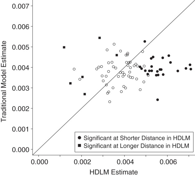
Scatterplot of assembly district-specific associations between convenience store availability within ½ mile (0.8 km) of schools and body mass index z scores of 7th grade students in California, 2001–2009. Associations estimated using the traditional model are shown on the y-axis, and those estimated from the hierarchical distributed-lag model (HDLM) are shown on the x-axis. Both models included school- and district-level random intercepts and slopes for time and spline time at the year 2005 and fixed coefficients for the averaged individual characteristics within schools. Black symbols represent assembly districts with significant associations at longer or shorter distances as identified in Figure 3. Data sources: 2001–2009 FitnessGram data for 7th grade children (California Department of Education) (28) and the National Establishments Time-Series database (30).

Additional adjustment for total student enrollment in a school, the percentage of children in a school that participated in the California school free or reduced-price meal program, and the percentage of adults with a bachelor's degree or higher residing in schools' census tracts resulted in attenuation of the DL coefficients, as might have been expected due to potential confounding and/or mediation (38, 39), and had a lower DIC of 59,831. However, there were still some ADs with DL coefficients that remained significant (See Web Figures 6 and 7).

DISCUSSION

To our knowledge, this was the first study to systematically evaluate differences in associations between the built environment and health across a large geographical area, namely the state of California. We used HDLMs to examine variability of the associations between convenience store availability around schools, a measure of the food environment, and children's BMIz averaged within schools. As expected, we found differences in the associations at the California AD level. Some ADs had associations approximately 2-fold higher than the overall mean, and there was some indication that the distances at which the associations were significant varied across districts. Our findings imply that the availability of convenience stores may matter for BMI only in some places, and at varying distances from schools. Our findings also raise the possibility that inconsistent evidence in the current literature may be due to the relationship itself varying across places. The observed variation in the convenience store–BMIz associations in this study was not spatially patterned across the state, suggesting that more localized environmental factors or policies may explain the observed differences across ADs. For example, unobserved variables that may modify the association across the state include open- versus closed-campus school policies, school bussing (which may limit exposure to poor food environments), street connectivity, walkability, and active transport to and from school, which may increase accessibility to convenience stores at longer or shorter distances from schools.

This study found that BMI–convenience store associations were strongest in urban and suburban ADs, although the relevant distances for the associations were greater in more central-city areas than suburban areas. Researchers have observed that youth living in urban areas are more likely to use active school transport (as opposed to passive transport, such as private vehicles) than their counterparts in rural and suburban areas (40, 41) and that users of active school transport have higher rates of corner-store purchasing before and after school than students using other methods of transportation (42). Thus, youth in more urban areas may have greater mobility, enabling them to access convenience stores at longer distances. In contrast, convenience stores at shorter distances may be more relevant for youth in less urban areas that have lower rates of active transport, who may access convenience stores during the school day to purchase food during lunch or recess.

Compared with a traditional multilevel model approach, the HDLM has several benefits and some limitations. While the traditional model requires a-priori specified distances (e.g., a ½-mile buffer) to construct measures of food stores around schools, the HDLM allows researchers to fully investigate how the food environment–health outcome association varies with distances from locations of interest. This approach provides more flexibility in the modeling of built environment predictors, particularly when the predictors may have associations with the outcome that vary with distance. The HDLM enables simultaneous examination of associations at various distances and is therefore particularly advantageous compared with traditional models, given that the current body of work in this area often lacks theory and empirical evidence to guide the selection of the appropriate buffer size. Although it is more complex, the HDLM enables us to begin to critically examine assumptions regarding the distances within which measures of the built environment are currently created. The HDLM also provides an approach to generate empirical evidence regarding relevant distances for built environment features that may differ according to broader characteristics of the environment and study participants (i.e., the uncertain geographic context problem). This may in turn add interpretability of associations observed across studies, and may enhance future research in this area.

The HDLM is inherently a more complex model than the traditional model; however, the HDLM has improved validity for estimating associations at predetermined buffer sizes. Specifically, the HDLM can be used to obtain accurate estimates of the association between built environment features at prespecified distances (e.g., within a ½-mile buffer) and health, whereas the traditional model can yield severely biased estimates, pointing away from the null, when the incorrect buffer size is chosen (13). Furthermore, given its flexibility, the HDLM can help improve knowledge (and/or generate hypotheses) about sources of variation in built environment associations across regions, particularly the distances within which built environment features may be more relevant for health outcomes. Similar to multilevel models, HDLMs can be extended to include spatially structured random intercepts and DL coefficients (43). In contrast to conventional multilevel models, it may be computationally intensive (but perhaps feasible) to further expand an HDLM to more levels of nesting, depending on the data size and structure and the number of levels.

There were limitations of the current study. Our analyses assumed that the built environment associations were the same across schools within a given AD, and the choice of ADs may still provide distinct results in comparison with studies using other areal units (census tracts or zip codes). We used census-tract-area measures of socioeconomic level as a proxy for the socioeconomic resources in school neighborhoods. This type of spatial interpolation may give rise to residual confounding, because the averaged value may not represent the resources closest to schools, particularly for large, heterogeneous census tracts. If socioeconomic indicators were available at very fine scales (e.g., street blocks), DL coefficients could also be used to model BMIz-SES associations in a similar fashion as for convenience stores. In urban areas where the convenience store–BMI association remained significant at longer distances, it is possible that the relationship between convenience store availability around schools and mean BMIz observed here may have captured associations with other environmental features (e.g., lack of supermarkets around children's homes). However, prior research found that children in urban areas purchased energy-dense, low-nutrient foods and sugary beverages from convenience stores before/after school and that these calories significantly contributed to children's dietary intakes, suggesting that convenience store availability en route to school could influence children's BMIs (5).

Future work should advance methods to improve our understanding of the complexity of the built environment and its potential associations with population health. New methods are needed that can incorporate the presence of multiple types of food outlets simultaneously, assess the relevance of different outlet types at different distances, and include variation in the associations across even more meaningful definitions of the broader environment in comparison with administrative areal units.

HDLM enables estimation of the underlying overall shape of food environment–health associations across a range of distances from locations of interest, as well as area-level heterogeneity of those associations across larger geographic areas. This approach serves to advance food environment–health research overall by helping to answer questions about whether, how, and in what places features of the built environment are associated with disease risk—questions regarding the uncertain geographic context problem and modifiable areal unit problem that have long been speculated about but seldom investigated systematically.

REFERENCES

- 1.Reilly JJ, Methven E, McDowell ZC et al. Health consequences of obesity. Arch Dis Child. 2003;889:748–752. [DOI] [PMC free article] [PubMed] [Google Scholar]
- 2.Reilly JJ, Kelly J. Long-term impact of overweight and obesity in childhood and adolescence on morbidity and premature mortality in adulthood: systematic review. Int J Obes (Lond). 2011;357:891–898. [DOI] [PubMed] [Google Scholar]
- 3.Daniels SR. The consequences of childhood overweight and obesity. Future Child. 2006;161:47–67. [DOI] [PubMed] [Google Scholar]
- 4.Sallis JF, Story M, Lou D. Study designs and analytic strategies for environmental and policy research on obesity, physical activity, and diet: recommendations from a meeting of experts. Am J Prev Med. 2009;36(2 suppl):S72–S77. [DOI] [PMC free article] [PubMed] [Google Scholar]
- 5.Borradaile KE, Sherman S, Vander Veur SS et al. Snacking in children: the role of urban corner stores. Pediatrics. 2009;1245:1293–1298. [DOI] [PubMed] [Google Scholar]
- 6.Gebauer H, Laska MN. Convenience stores surrounding urban schools: an assessment of healthy food availability, advertising, and product placement. J Urban Health. 2011;884:616–622. [DOI] [PMC free article] [PubMed] [Google Scholar]
- 7.Hillier A, Cole BL, Smith TE et al. Clustering of unhealthy outdoor advertisements around child-serving institutions: a comparison of three cities. Health Place. 2009;154:935–945. [DOI] [PubMed] [Google Scholar]
- 8.Rahman T, Cushing RA, Jackson RJ. Contributions of built environment to childhood obesity. Mt Sinai J Med. 2011;781:49–57. [DOI] [PubMed] [Google Scholar]
- 9.Sallis JF, Glanz K. The role of built environments in physical activity, eating, and obesity in childhood. Future Child. 2006;161:89–108. [DOI] [PubMed] [Google Scholar]
- 10.Kipke MD, Iverson E, Moore D et al. Food and park environments: neighborhood-level risks for childhood obesity in East Los Angeles. J Adolesc Health. 2007;404:325–333. [DOI] [PubMed] [Google Scholar]
- 11.Singh GK, Siahpush M, Kogan MD. Neighborhood socioeconomic conditions, built environments, and childhood obesity. Health Aff (Millwood). 2010;293:503–512. [DOI] [PubMed] [Google Scholar]
- 12.Black JL, Macinko J. Neighborhoods and obesity. Nutr Rev. 2008;661:2–20. [DOI] [PubMed] [Google Scholar]
- 13.Schaefer-McDaniel N, Caughy MO, O'Campo P et al. Examining methodological details of neighbourhood observations and the relationship to health: a literature review. Soc Sci Med. 2010;702:277–292. [DOI] [PubMed] [Google Scholar]
- 14.Fotheringham AS, Wong DWS. The modifiable areal unit problem in multivariate statistical analysis. Environ Plann A. 1991;237:1025–1044. [Google Scholar]
- 15.Openshaw S. Developing GIS-relevant zone-based spatial analysis methods. In: Longley P, Batty M, eds. Spatial Analysis: Modelling in a GIS Environment. New York, NY: John Wiley & Sons, Inc.; 1996:55–73. [Google Scholar]
- 16.Spielman SE, Yoo E-H. The spatial dimensions of neighborhood effects. Soc Sci Med. 2009;686:1098–1105. [DOI] [PubMed] [Google Scholar]
- 17.Baek J, Sánchez BN, Berrocal VJ et al. Distributed lag models: examining associations between the built environment and health. Epidemiology. 2016;271:116–124. [DOI] [PMC free article] [PubMed] [Google Scholar]
- 18.Kwan M-P. The uncertain geographic context problem. Ann Assoc Am Geogr. 2012;1025:958–968. [Google Scholar]
- 19. California Center for Public Health Advocacy. Searching for healthy food: the food landscape in California cities and counties. http://www.publichealthadvocacy.org/searchingforhealthyfood.html Published January 19, 2007. Accessed December 15, 2014.
- 20. California State Assembly. Your legislature. http://assembly.ca.gov/sites/assembly.ca.gov/files/2013-14_CaliforniaAsmPamphlet.pdf Published March, 2013. Accessed September 16, 2014.
- 21.Dominici F, Samet JM, Zeger SL et al. Hierarchical modelling strategy combining evidence on air pollution and daily mortality from the 20 largest US cities: a hierarchical modelling strategy. J R Stat Soc Ser A Stat Soc. 2000;1633:263–302. [Google Scholar]
- 22.Berhane K, Thomas DC. A two-stage model for multiple time series data of counts. Biostatistics. 2002;31:21–32. [DOI] [PubMed] [Google Scholar]
- 23.Huang Y, Dominici F, Bell ML. Bayesian hierarchical distributed lag models for summer ozone exposure and cardio-respiratory mortality. Environmetrics. 2005;165:547–562. [DOI] [PMC free article] [PubMed] [Google Scholar]
- 24.Rondeau V, Berhane K, Thomas DC. A three-level model for binary time-series data: the effects of air pollution on school absences in the Southern California Children's Health Study. Stat Med. 2005;247:1103–1115. [DOI] [PubMed] [Google Scholar]
- 25.Peng RD, Dominici F, Welty LJ. A Bayesian hierarchical distributed lag model for estimating the time course of risk of hospitalization associated with particulate matter air pollution. J R Stat Soc Ser C Appl Stat. 2009;581:3–24. [Google Scholar]
- 26.Madden LV, Paul PA. An assessment of mixed-modeling approaches for characterizing profiles of time-varying response and predictor variables. Phytopathology. 2010;10010:1015–1029. [DOI] [PubMed] [Google Scholar]
- 27.Zhao X, Chen F, Feng Z et al. The temporal lagged association between meteorological factors and malaria in 30 counties in south-west China: a multilevel distributed lag non-linear analysis. Malar J. 2014;13:57. [DOI] [PMC free article] [PubMed] [Google Scholar]
- 28. California Department of Education. Physical fitness testing (PFT). http://www.cde.ca.gov/ta/tg/pf/. Reviewed November 20, 2015. Accessed October 1, 2014. [Google Scholar]
- 29. Centers for Disease Control and Prevention. A SAS program for the 2000 CDC growth charts (ages 0 to <20 years). http://www.cdc.gov/nccdphp/dnpao/growthcharts/resources/sas.htm Published 2005. Accessed September 15, 2014. [Google Scholar]
- 30. Business Dynamics Research Consortium. National Establishment Time-Series (NETS) Database: 2012 Database Description. Denver, CO: Walls & Associates; 2013. http://exceptionalgrowth.org/downloads/NETSDatabaseDescription2013.pdf. Accessed April 5, 2015. [Google Scholar]
- 31. Berkeley Law, Center for Research. 2001 assembly districts [ArcGIS file] In: Statewide Database http://statewidedatabase.org/geography.html Published 2014. Accessed July 13, 2014.
- 32.Sanchez-Vaznaugh EV, Sánchez BN, Baek J et al. ‘Competitive’ food and beverage policies: are they influencing childhood overweight trends? Health Aff (Millwood). 2010;293:436–446. [DOI] [PubMed] [Google Scholar]
- 33.Hastie TJ, Tibshirani RJ. Generalized Additive Models. Boca Raton, FL: CRC Press; 1990. [Google Scholar]
- 34.Zanobetti A, Wand MP, Schwartz J et al. Generalized additive distributed lag models: quantifying mortality displacement. Biostatistics. 2000;13:279–292. [DOI] [PubMed] [Google Scholar]
- 35.Spiegelhalter DJ, Best NG, Carlin BP et al. Bayesian measures of model complexity and fit. J R Stat Soc Series B Stat Methodol. 2002;644:583–639. [Google Scholar]
- 36.Clayton D, Kaldor J. Empirical Bayes estimates of age-standardized relative risks for use in disease mapping. Biometrics. 1987;433:671–681. [PubMed] [Google Scholar]
- 37.Besag J, York J, Mollié A. Bayesian image restoration, with two applications in spatial statistics. Ann Inst Stat Math. 1991;431:1–20. [Google Scholar]
- 38.Chaix B, Leal C, Evans D. Neighborhood-level confounding in epidemiologic studies: unavoidable challenges, uncertain solutions. Epidemiology. 2010;211:124–127. [DOI] [PubMed] [Google Scholar]
- 39.Diez Roux AV. Estimating neighborhood health effects: the challenges of causal inference in a complex world. Soc Sci Med. 2004;5810:1953–1960. [DOI] [PubMed] [Google Scholar]
- 40.Babey SH, Hastert TA, Huang W et al. Sociodemographic, family, and environmental factors associated with active commuting to school among US adolescents. J Public Health Policy. 2009;30(suppl 1):S203–S220. [DOI] [PubMed] [Google Scholar]
- 41.Yang Y, Diez Roux AV, Bingham CR. Variability and seasonality of active transportation in USA: evidence from the 2001 NHTS. Int J Behav Nutr Phys Act. 2011;8:96. [DOI] [PMC free article] [PubMed] [Google Scholar]
- 42.Vander Veur SS, Sherman SB, Lent MR et al. Corner store and commuting patterns of low-income, urban elementary school students. Curr Urban Stud. 2013;14:166–170. [Google Scholar]
- 43.MacNab YC, Gustafson P. Regression B-spline smoothing in Bayesian disease mapping: with an application to patient safety surveillance. Stat Med. 2007;2624:4455–4474. [DOI] [PubMed] [Google Scholar]
Associated Data
This section collects any data citations, data availability statements, or supplementary materials included in this article.