False Appearance of Gene–Environment Interactions in Genetic Association Studies

Supplemental Digital Content is available in the text

Abstract

Under the assumption of gene–environment independence, unknown/unmeasured environmental factors, irrespective of what they may be, cannot confound the genetic effects. This may lead many people to believe that genetic heterogeneity across different levels of the studied environmental exposure should only mean gene–environment interaction—even though other environmental factors are not adjusted for. However, this is not true if the odds ratio is the effect measure used for quantifying genetic effects. This is because the odds ratio is a “noncollapsible” measure—a marginal odds ratio is not a weighted average of the conditional odds ratios, but instead has a tendency toward the null. In this study, the authors derive formulae for gene–environment interaction bias due to noncollapsibility. They use computer simulation and real data example to show that the bias can be substantial for common diseases. For genetic association study of nonrare diseases, researchers are advised to use collapsible measures, such as risk ratio or peril ratio.

INTRODUCTION

The occurrences of most human diseases are the result of complex interplay between genes and environmental exposures. In genetic association studies nowadays, it has become a common practice for researchers to examine any possible interaction between genes and environmental exposures, in addition to their respective independent effects.^1–5

For any person, his/her genes are constitutional (determined from birth), and environmental exposures, exogenous (acquired throughout life), and therefore the assumption of gene–environment independence is often tenable among the nondiseased subjects in the study population.^6–9 Under the assumption, unknown/unmeasured environmental factors will not confound genetic main effects. Taking a step further, one will believe that a simple stratified analysis which shows heterogeneous genetic effects across different levels of the environmental exposure under study is all that is needed to demonstrate gene–environment interaction—there is no need to further stratify on the levels of other environmental factors, because no matter what they are they will not confound the stratum-specific genetic effects in the study anyway.

Unfortunately, this is not true if the odds ratio is the effect measure used for quantifying genetic effects. Odds ratios are well known to be “noncollapsible,” that is, a marginal odds ratio, even without confounding, is not a weighted average of the conditional (stratum-specific) odds ratios, but instead has a tendency toward the null.^10–17 Hernán et al put it this way: “... a quantitative difference between conditional and marginal odds ratios in the absence of confounding is a mathematical oddity (no pun intended), not a reflection of bias.”¹⁶ It is less well recognized, though, that the odd behavior of the odds ratios (again no pun intended) can cause trouble: the stratum-specific genetic odds ratios may be homogeneous at first, but because of the noncollapsibility property they move toward the null to different degrees and appear heterogeneous in different levels of the environmental exposure, creating a false appearance of gene–environment interaction.

In this study, we derive formulae for gene–environment interaction bias due to noncollapsibility. We use computer simulation and real data example to show that the bias can be substantial for common diseases.

METHODS

Assume that the following 3 binary factors are associated with the disease under study (D): a gene (G) with an odds ratio of disease association of OR_GD, an environmental exposure (E) with OR_ED, and an unknown/unmeasured factor (U) with OR_UD, respectively. We assume that E and U (both are environmental factors) are independent of G (gene–environment independence). The E and U themselves can be independent of each other (OR_EU = 1, as in Figure 1A where U is an independent risk factor for D), or are associated (OR_EU ≠ 1, as in Figure 1B where U is a mediator, and 1C where U is a confounder, of the relation between E and D). In addition, we assume no interaction between any of them.

FIGURE 1.

Causal diagrams showing the relations between G (genetic factor), E (environmental factor), U (unknown/unmeasured factor), and D (disease).

Because U is unmeasured, the researchers can only stratify on E to obtain the stratum-specific odds ratios of disease association for G: the OR_GD|E=1 in the E = 1 stratum, and the OR_GD|E=0 in the E = 0 stratum, respectively. To quantify the extent of heterogeneity of the genetic odds ratios across the levels of E, we calculate the percent discrepancy between OR_GD|E=1 and OR_GD|E=0: 

A larger value of percent discrepancy means greater heterogeneity, and greater gene–environment interaction bias. (Here we assume no interaction, so a discrepancy between the 2 stratum-specific genetic odds ratios indicates bias.)

Percent discrepancy is a function of OR_GD|E=1 and OR_GD|E=0, which in turns are functions of OR_GD,OR_ED,OR_UD,OR_EU and the prevalence of D, G, E, and U. The formulas appear rather cumbersome and are relegated to Web Appendix 1, where we have taken into account the 3 possible relations between E and U: (I) E and U are independent of each other, (II) E and U are associated: U is a mediator, and (III) E and U are associated: U is a confounder. Web Appendix 2, derives a condition when an unmeasured mediator and an unmeasured confounder produce the same magnitude of bias (as quantified by the index of percent discrepancy).

The probability of making a false alarm of gene–environment interaction (i.e., the type I error rate, because we assume no interaction) is a function of the sample size and the above parameters. This probability is difficult to derive analytically but should be fairly easy to estimate using Monte Carlo simulations. To be precise, data is generated according to the parameter values given and the sample size specified. The simulated data is to be analyzed using the model log(Odds)∼G + E + G × E. [The true disease model is log(Odds)∼G + E + U. But because U is unmeasured, the model does not contain a U term, and because the gene–environment interaction is of interest, the model explicitly contains a G × E term.] The type I error rate is calculated as the proportion of the simulations with the P value of the G × E interaction term less than the significance level (α level).

Web Appendix 3, presents a function (apparent.interaction) written in R code. Input the relevant parameters and the sample sizes as the arguments to the function, it will output the percent discrepancy and the type I error rate automatically.

Ethical approval is not necessary for the following data used in this study: computer generated data (simulation study) and parameter values taken from published papers (real data application).

RESULTS

A Small-Scale Simulation Study

Figure 2 shows the values of percent discrepancy under different scenarios when P_G (allele frequency) is 0.3, P_E (exposure prevalence) is 0.2, P_U (prevalence of the unmeasured factor) is 0.5, and OR_GD is 4. We consider the situations when OR_EU = 1 (E is independent of U) and OR_EU = 5 (E and U are associated; this can either mean that U is a mediator or a confounder, see Web Appendix 2). When E is independent of U (dotted lines), the percent discrepancy is absolutely zero for either OR_ED = 1 (panels a, d, and g) or OR_UD = 1 (panels a, b, and c). When E and U are associated (dashed lines), the value can be nonzero even with OR_ED = 1. If both OR_ED>1 and OR_UD>1 (panels e, f, h, and i), the percent discrepancy increases as disease prevalence increases. When OR_ED = OR_UD = 10 (panel i), the value increases from 5% to 10% (disease prevalence = 0.001) to ∼20% (disease prevalence = 0.01).

FIGURE 2.

Percent discrepancy under various scenarios [A:(OR_ED, OR_UD,) = (1,1); B:(OR_ED, OR_UD,) = (5,1); C:(OR_ED, OR_UD,) = (10,1); D:(OR_ED, OR_UD,) = (1,5); E:(OR_ED, OR_UD,) = (5.5); F:(OR_ED, OR_UD,) = (10,5); G:(OR_ED, OR_UD,) = (1,10); H:(OR_ED, OR_UD,) = (5,10); I:(OR_ED, OR_UD,) = (10,10); dotted lines: E is independent of U; dashed lines: E is associated with U]. OR = odds ratio.

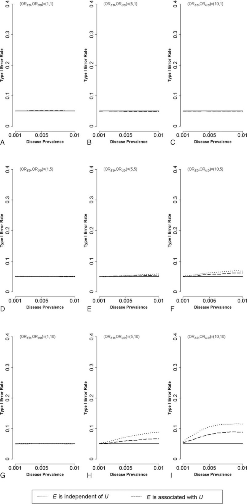
The type I error rates (based on 100,000 simulations) for the gene–environment interaction under the same scenarios depicted in Figure 2 are presented in Figures 3 (small sample size; case = 250, control = 250), 4 (moderate; 500, 500), and 5 (large; 2500, 2500), respectively. With a small sample size (Figure 3), the type I error rate is roughly at around the control value of α = 0.05 when the disease prevalence is lower. When the disease prevalence becomes higher and if OR_ED>1 and OR_UD>1, the type I error rate is slightly elevated but remains <0.1. With a moderate sample size (Figure 4), the inflation of the type I error rate then becomes more severe (exceeding 0.1 at times). With a large sample size (Figure 5), the inflation problem becomes intolerable. The type I error rate can go so high as to ∼0.4 for common disease (disease prevalence = 0.01); moreover, this inflation problem is non-negligible even for rare disease (disease prevalence = 0.001).

FIGURE 3.

Type I error rate for the gene–environment interaction in case-control studies with small sample size (n = 500) [A:(OR_ED, OR_UD,) = (1,1); B:(OR_ED, OR_UD,) = (5,1); C:(OR_ED, OR_UD,) = (10,1); D:(OR_ED, OR_UD,) = (1,5); E:(OR_ED, OR_UD,) = (5,5); F:(OR_ED, OR_UD,) = (10,5); G:(OR_ED, OR_UD,) = (1,10); H:(OR_ED, OR_UD,) = (5,10); I:(OR_ED, OR_UD,) = (10,10); dotted lines: E is independent of U; dashed lines: E is associated with U]. OR = odds ratio.

FIGURE 4.

Type I error rate for the gene–environment interaction in case-control studies with moderate sample size (n = 1000) [A:(OR_ED, OR_UD,) = (1,1); B:(OR_ED, OR_UD,) = (5,1); C:(OR_ED, OR_UD,) = (10,1); D:(OR_ED, OR_UD,) = (1,5); E:(OR_ED, OR_UD,) = (5,5); F:(OR_ED, OR_UD,) = (10,5); G:(OR_ED, OR_UD,) = (1,10); H:(OR_ED, OR_UD,) = (5,10); I:(OR_ED, OR_UD,) = (10,10); dotted lines: E is independent of U; dashed lines: E is associated with U]. OR = odds ratio.

FIGURE 5.

Type I error rate for the gene–environment interaction in case-control studies with large sample size (n = 5000) [A:(OR_ED, OR_UD,) = (1,1); B:(OR_ED, OR_UD,) = (5,1); C:(OR_ED, OR_UD,) = (10,1); D:(OR_ED, OR_UD,) = (1,5); E:(OR_ED, OR_UD,) = (5,5); F:(OR_ED, OR_UD,) = (10,5); G:(OR_ED, OR_UD,) = (1,10); H:(OR_ED, OR_UD,) = (5,10); I:(OR_ED, OR_UD,) = (10,10); dotted lines: E is independent of U; dashed lines: E is associated with U]. OR = odds ratio.

Similar results can be found when P_G = 0.5, P_E = 0.2, P_U = 0.5, and OR_GD = 4 (Web Appendix 4) and when P_G = 0.3, P_E = 0.2, P_U = 0.5 and OR_GD = 2 (Web Appendix 5). We also perform a logistic regression analysis with all the G, E, and U (assuming U is indeed measured) included in the model: log(Odds)∼G + E + U + G × E. The type I error rates for the G × E interaction are now close to 0.05 as expected (results not shown).

A Real Data Application

Age-related macular degeneration (AMD) is a common disease among the elderly population, with a prevalence of around 1.5 %.¹⁸ Documented risk factors for the disease include the component factor H (CFH) gene and cigarette smoking, both with disease odds ratios of around 5.^19,20 A small study suggested that heavy alcohol use is a risk factor for AMD and the odd ratio can be up to ∼10.²¹ However, the finding is inconsistent in other studies.^19,22

Assume that a case-control study for AMD does not measure alcohol use—it will not confound the genetic main effects anyway under the gene–environment independence assumption. The question now is whether that unmeasured factor will confound our analysis of possible gene–environment interaction between CFH gene and smoking.

We input the following parameters and sample sizes to the R function we developed (Web Appendix 3): OR_GD = 5, OR_ED = 5, OR_UD = 10, P_D = 0.015, P_G = 0.25 (allele frequency),²⁰ P_E = 0.25 (smoking prevalence),²³ OR_EU = 5 (odds ratio between smoking and drinking),²⁴ and sample size = 1000 and 5000, respectively. The results are as follows: percent discrepancy = 14.8%, type I error rate = 0.075 (sample size = 1000), and 0.173 (sample size = 5000). From these, we see that a large sized case-control study for AMD, without a proper adjustment for alcohol use, will be liable to reach an erroneous conclusion about the CFH gene × smoking interaction.

DISCUSSION

The literature documented 2 genuine no-interaction scenarios where apparent interaction can nonetheless arise, that is, across different strata there exists: (1) varying measurement errors, or (2) varying confounding effects.^25–29 In either case, the stratum-specific effect measures can be biased to varying degrees across different strata. Such heterogeneity in stratum-specific effect measures naturally will lead a well-trained epidemiologist to contemplate an interaction (while there is actually none). This study demonstrates that varying noncollapsibility (across different levels of the environmental factor under study) in its own right can also produce apparent interaction.

Vanderweele et al considered only the rare-disease scenarios (where odds ratios approximate risk ratios, and hence are collapsible) and concluded that “... under gene–environment independence, the only way to have a nonzero interaction parameter is for some form of gene–environment interaction to be present, either with the environmental factor of interest or with some confounder of it.”³⁰ For diseases that are more common, our study suggests otherwise. We show that for nonrare diseases, the apparent gene–environment interaction can and will arise, even if the gene of interest is not associated with, and is not interacting with, the environmental factor under study and any other unmeasured environmental factor.

This study also shows that using the noncollapsible odds ratios, the probability of making a false alarm of gene–environment interaction (inflation of the type I error rate) increases with increasing sample sizes. This is as expected because a bias arising from noncollapsibility, however small it may be, can easily become significant in big studies. This also warns against a fishing expedition in search of gene–environment interactions in a large genetic association study, unless all strong environmental factors have been measured and adjusted for in the study, be they independent risk factors, mediators, or confounders (which is of course next to impossible).

Based on the findings of this study, in genetic association studies of nonrare diseases we advise researchers to use collapsible measures, such as the risk ratio or the peril ratio.^31,32 Web Appendix 6 (for risk ratio) and Web Appendix 7 (for the peril ratio) show that these 2 indices will not lead us astray regarding the gene–environment interaction in the presence of unknown/unmeasured environmental variables. Using the peril ratio index^31,32 in particular, researchers have the additional advantage of being able to test for gene–environment interactions under the sufficient component cause model directly. A hybrid (part case-control, part cohort) design, the “case-base” study, readily produces risk ratio (or peril ratio) estimates without resorting to the rare-disease assumption.³³

REFERENCES

- 1.Cordell HJ. Estimation and testing of gene–environment interactions in family-based association studies. Genomics 2009; 93:5–9. [DOI] [PMC free article] [PubMed] [Google Scholar]
- 2.Hunter DJ. Gene–environment interactions in human diseases. Nat Rev Genet 2005; 6:287–298. [DOI] [PubMed] [Google Scholar]
- 3.Le Marchand L, Wilkens LR. Design considerations for genomic association studies: importance of gene–environment interactions. Cancer Epidemiol Biomarkers Prev 2008; 17:263–267. [DOI] [PubMed] [Google Scholar]
- 4.Lewis CM, Knight J. Introduction to genetic association studies. Cold Spring Harb Protoc 2012; 2012:297–306. [DOI] [PubMed] [Google Scholar]
- 5.Rava M, Ahmed I, Demenais F, et al. Selection of genes for gene–environment interaction studies: a candidate pathway-based strategy using asthma as an example. Environ Health 2013; 12:56. [DOI] [PMC free article] [PubMed] [Google Scholar]
- 6.Chatterjee N, Carroll RJ. Semiparametric maximum likelihood estimation exploiting gene–environment independence in case-control studies. Biometrika 2005; 92:399–418. [Google Scholar]
- 7.Chui TTT, Lee WC. Estimating risks and relative risks in case-base studies under the assumptions of gene–environment independence and Hardy-Weinberg equilibrium. PLoS One 2014; 9:e105398. [DOI] [PMC free article] [PubMed] [Google Scholar]
- 8.Lee WC, Wang LY, Cheng KF. An easy-to-implement approach for analyzing case-control and case-only studies assuming gene–environment independence and Hardy-Weinberg equilibrium. Stat Med 2010; 29:2557–2567. [DOI] [PubMed] [Google Scholar]
- 9.Lee WC. Testing for sufficient-cause gene–environment interactions under independence and Hardy-Weinberg equilibrium assumptions. Am J Epidemiol 2015; 182:9–16. [DOI] [PubMed] [Google Scholar]
- 10.Neuhaus JM, Jewell NP. A geometric approach to assess bias due to omitted covariates in generalized linear models. Biometrika 1993; 80:807–815. [Google Scholar]
- 11.Greenland S, Robins JM, Pearl J. Confounding and collapsibility in causal inference. Stat Sci 1999; 14:29–46. [Google Scholar]
- 12.Doi M, Nakamura T, Yiimamoto E. Conservative tendency of the crude odds ratio. J Japan Statist Soc 2001; 31:53–65. [Google Scholar]
- 13.Cummings P. The relative merits of risk ratios and odds ratios. Arch Pediatr Adolesc Med 2009; 163:438–445. [DOI] [PubMed] [Google Scholar]
- 14.Kent DM, Trikalinos TA, Hill MD. Are unadjusted analyses of clinical trials inappropriately biased toward the null? Stroke 2009; 40:672–673. [DOI] [PMC free article] [PubMed] [Google Scholar]
- 15.Groenwold RH, Moons KG, Peelen LM, et al. Reporting of treatment effects from randomized trials: a plea for multivariable risk ratios. Contemp Clin Trials 2011; 32:399–402. [DOI] [PubMed] [Google Scholar]
- 16.Hernán MA, Clayton D, Keiding N. The Simpson's paradox unraveled. Int J Epidemiol 2011; 40:780–785. [DOI] [PMC free article] [PubMed] [Google Scholar]
- 17.Pang M, Kaufman JS, Platt RW. Studying noncollapsibility of the odds ratio with marginal structural and logistic regression models. Stat Methods Med Res 2013; DOI:10/1177/0962280213505804. [DOI] [PubMed] [Google Scholar]
- 18.Friedman DS, O’Colmain BJ, Munoz B, et al. Prevalence of age-related macular degeneration in the United States. Arch Ophthalmol 2004; 122:564–572. [DOI] [PubMed] [Google Scholar]
- 19.Giudice GL. Age-Related Macular Degeneration—Etiology, Diagnosis and Management—A Glance at the Future. Vienna: InTech; 2013. [Google Scholar]
- 20.Klein RJ, Zeiss C, Chew EY, et al. Complement factor H polymorphism in age-related macular degeneration. Science 2005; 308:385–389. [DOI] [PMC free article] [PubMed] [Google Scholar]
- 21.Fraser-Bell S, Wu J, Klein R, et al. Smoking, alcohol intake, estrogen use, and age-related macular degeneration in Latinos: the Los Angeles Latino Eye Study. Am J Ophthalmol 2006; 141:79–87. [DOI] [PubMed] [Google Scholar]
- 22.Adams MK, Chong EW, Williamson E, et al. 20/20—Alcohol and age-related macular degeneration: the Melbourne Collaborative Cohort Study. Am J Epidemiol 2012; 176:289–298. [DOI] [PubMed] [Google Scholar]
- 23.Jamal A, Agaku IT, O’Connor E, et al. Current cigarette smoking among adults—United States, 2005–2013. MMWR Morb Mortal Wkly Rep 2014; 63:1108–1112. [PMC free article] [PubMed] [Google Scholar]
- 24.De Leon J, Rendon DM, Baca-Garcia E, et al. Association between smoking and alcohol use in the general population: stable and unstable odds ratios across two years in two different countries. Alcohol Alcohol 2007; 42:252–257. [DOI] [PubMed] [Google Scholar]
- 25.Greenland S. The effect of misclassification in the presence of covariates. Am J Epidemiol 1980; 112:564–569. [DOI] [PubMed] [Google Scholar]
- 26.Greenland S, Robins JM. Confounding and misclassification. Am J Epidemiol 1985; 122:495–506. [DOI] [PubMed] [Google Scholar]
- 27.Rothman KJ, Lash TL, Greenland S. Modern Epidemiology. 3rd edPhiladelphia, PA: Lippincott Williams & Wilkins; 2012. [Google Scholar]
- 28.Szklo M, Nieto J. Epidemiology: Beyond the Basics. 3rd ed.Burlington, MA: Jones & Bartlett Learning; 2012. [Google Scholar]
- 29.Zhang L, Mukherjee B, Ghosh M, et al. Accounting for error due to misclassification of exposures in case-control studies of gene–environment interaction. Stat Med 2008; 27:2756–2783. [DOI] [PubMed] [Google Scholar]
- 30.Vanderweele TJ, Ko YA, Mukherjee B. Environmental confounding in gene–environment interaction studies. Am J Epidemiol 2013; 178:144–152. [DOI] [PMC free article] [PubMed] [Google Scholar]
- 31.Lee WC. Assessing causal mechanistic interactions: a peril ratio index of synergy based on multiplicativity. PLoS One 2013; 8:e67424. [DOI] [PMC free article] [PubMed] [Google Scholar]
- 32.Lee WC. Estimation of a common effect parameter from follow-up data when there is no mechanistic interaction. PLoS One 2014; 9:e86374. [DOI] [PMC free article] [PubMed] [Google Scholar]
- 33.Chui TTT, Lee WC. A regression-based method for estimating risks and relative risks in case-base studies. PLoS One 2013; 8:e83275. [DOI] [PMC free article] [PubMed] [Google Scholar]
Associated Data
This section collects any data citations, data availability statements, or supplementary materials included in this article.