Extracting information from previous full-dose CT scan for knowledge-based Bayesian reconstruction of current low-dose CT images

Abstract

Markov random field (MRF) model has been widely employed in edge-preserving regional noise smoothing penalty to reconstruct piece-wise smooth images in the presence of noise, such as in low-dose computed tomography (LdCT). While it preserves edge sharpness, its regional smoothing may sacrifice tissue image textures, which have been recognized as useful imaging biomarkers, and thus it may compromise clinical tasks such as differentiating malignant vs. benign lesions, e.g., lung nodules or colon polyps. This study aims to shift the edge-preserving regional noise smoothing paradigm to texture-preserving framework for LdCT image reconstruction while retaining the advantage of MRF’s neighborhood system on edge preservation. Specifically, we adapted the MRF model to incorporate the image textures of muscle, fat, bone, lung, etc. from previous full-dose CT (FdCT) scan as a priori knowledge for texture-preserving Bayesian reconstruction of current LdCT images. To show the feasibility of the proposed reconstruction framework, experiments using clinical patient scans were conducted. The experimental outcomes showed a dramatic gain by the a priori knowledge for LdCT image reconstruction using the commonly-used Haralick texture measures. Thus, it is conjectured that the texture-preserving LdCT reconstruction has advantages over the edge-preserving regional smoothing paradigm for texture-specific clinical applications.

I. Introduction

X-RAY computed tomography (CT) has been widely exploited for various clinical applications. However, CT scan is a radiation-intensive procedure [1, 2]. For image-guided interventions and dynamical studies where repeated scans are routinely prescribed, the accumulated CT radiation dose could be tremendous. For instance, CT is commonly used to guide a needle for lung nodule biopsy [3], where up to ten scans could be performed on the same patient. Similar situation occurs to dynamical scans in order to assess disease stages [4]. To reduce radiation dose, a full-dose (i.e., diagnostic high-quality) CT scan can be first performed to set up a reference as current practice does, but the following scanning series may be acquired at lower dose levels by lowering the production of X-ray tube current and exposure time (milliampere-second (mAs)) during data acquisition without hardware modification, followed by an adaptive software approach for statistical image reconstruction (SIR) to control the increased data noise [5, 6]. In the past decade, many SIR algorithms have been developed to incorporate the physics and geometry of CT imaging. The central theme of these developed SIR algorithms is based on the assumption that the image intensity distribution shall be piece-wise smooth, so various regularizations have been explored to realize a piece-wise smooth image reconstruction with consistency to the acquired low-dose projection data [6–8].

More recently, noticeable research efforts have been devoted to take advantage of previously-available FdCT scan, in addition to the above assumption, for the purpose of improving the piece-wise smooth image reconstruction of low-dose CT (LdCT) images [9–16]. For instance, Nett et al. [9] incorporated a registered FdCT image into their prior image constrained compressed sensing (PICCS) cost function [17] for iterative reconstruction of subsequent LdCT images. Stayman et al. [14, 15] presented a PICCS-type penalty term, but the high-quality prior image was formulated into a joint estimation framework for both image registration and image reconstruction in order to better capturing the anatomical motion among different scans. Moreover, Ma et al. [11, 16] proposed previous FdCT image induced nonlocal means penalties to improve the following LdCT image reconstruction for perfusion and interventional imaging, wherein the previous FdCT image was also pre-registered with the LdCT scans. These efforts share the common idea of registering the FdCT image structure with the LdCT image to ensure piece-wise regional smoothness and edge-sharpness image reconstructions. The edge-preserving regional smoothing paradigm can sharpen the tissue region borders, but may sacrifice the tissue region image texture characteristics, which have been shown as a useful imaging marker for many clinical tasks, e.g., [18–20].

This exploratory study aims to shift the paradigm to texture-preserving LdCT reconstruction by capturing the regional tissue textures from the previous FdCT scan and incorporating the textures as a priori knowledge for Bayesian reconstruction of the current LdCT images. Specifically, it captures the image textures of muscle, fat, bone, lung, etc., from the full-dose image and then incorporates the tissue image textures as a priori knowledge for Bayesian reconstruction of the corresponding tissue regions in the low-dose images, so that the reconstruction preserves not only the edges but also the textures inside the tissue regions. It is noted that several other studies also expressed interest on image texture preservation in iterative reconstruction [21, 22].

The remainder of this paper is organized as follows. Section II reviews the Bayesian theorem-based SIR framework and introduces a texture penalty model to incorporate tissue textures from the full-dose scan. Section III describes experimental design using both simulated and acquired low-dose projection data of patients, and then reports the performance of the presented knowledge-based Bayesian reconstruction with the texture penalty model. After a brief discussion, conclusions of this study are drawn in Section IV.

II. Methods

A. Bayesian Theorem-based Texture-preserving Low-dose CT Image Reconstruction

Given a set of acquired projection data, denoted by a vector $\mathbf{y}\in {\Re }^{I\times 1}$, where I is the number of data elements, we are interested in a solution, denoted by a vector $\mathbf{\mu }\in {\Re }^{J\times 1}$, where J is the number of image voxels, which maximizes the posterior probability $\mathrm{p}(\mathbf{\mu }|\mathbf{y})$. By the Bayesian theorem, we have:

$$p(\mathbf{\mu }|\mathbf{y})=p(\mathbf{y}|\mathbf{\mu })p(\mathbf{\mu })/p(\mathbf{y})\approx p(\mathbf{y}|\mathbf{\mu })p(\mathbf{\mu })$$ (1)

where $\mathrm{p}(\mathbf{y})$ becomes a constant when maximizing the posterior probability and, therefore, is ignored. Let the log data likelihood or fidelity term, $\log \mathrm{p}(\mathbf{y}|\mathbf{\mu })$, be described as a re-weighted least squares (RWLS) [6] and the log prior term, $\log \mathrm{p}(\mathbf{\mu })$, be described by a Markov random field (MRF) model [23], the desired solution can be expressed as:

$${\mathbf{\mu }}^{\ast }=\underset{\mathbf{\mu }}{{\displaystyle \text{arg min}}}\left\{{(\mathbf{y}-\mathbf{A}\mathbf{\mu })}^{T}D(\mathbf{y}-\mathbf{A}\mathbf{\mu })+\beta U(\mathbf{\mu })\right\}$$ (2)

where A is the projection matrix with size I×J, and its element ${\mathbf{A}}_{\mathit{ij}}$ is calculated as the intersection length of projection ray i with voxel j. $\mathbf{A}\mathbf{\mu }$ denotes the mean value vector $\overline{y}$ of the acquired data y. T is a transpose operator. Since the noise, i.e., the difference $(\mathbf{y}-\mathbf{A}\mathbf{\mu })$, is statistically independent among all the data elements, D is a diagonal matrix, where each diagonal element is called a weight for its corresponding datum. Because of the Poisson nature in X-ray generation and detection, each weight in D must depend on the corresponding mean $\mathbf{A}\mathbf{\mu }$ [24, 25] and the weight D must be re-weighted in calculating the solution of Eq. (2), thus the first term of Eq. (2) is called RWLS. A mathematical derivation for D is given in [26]. $\mathrm{U}(\mathbf{\mu })$ in the second term of Eq. (2), based on the MRF model [23], can be expressed as:

$$U(\mathbf{\mu })={\displaystyle \sum _j{\displaystyle \sum _{m\in W_j}{w}_{\mathit{jm}}\varphi ({\mu }_j-{\mu }_m)}}$$ (3)

where index j runs over all the voxels in the image domain, W_j denotes a small fixed neighborhood window (typically 8 neighbors in a 2D case) of the jth image voxel, and w_jm is the weighting coefficient that indicates the interaction degree between voxel j and voxel m. Usually the weighting coefficient is considered to be inversely proportional to the Euclidean distance between the two voxels. Thus, in 2D case, w_jm for the eight neighboring image pixels can be given as:

$$\left[\begin{array}{ccc}0.104& 0.146& 0.104\\ 0.146& 0& 0.146\\ 0.104& 0.146& 0.104\end{array}\right]$$

And ϕ denotes a potential function, which can be given as:

$$\varphi (\mathrm{\Delta })={\mathrm{\Delta }}^2,\text{or}\varphi (\mathrm{\Delta })=\{\begin{array}{ll}{\mathrm{\Delta }}^2\hfill & \left|\mathrm{\Delta }\right|\le \delta \hfill \\ 2\delta \left|\mathrm{\Delta }\right|-{\delta }^2\hfill & \left|\mathrm{\Delta }\right|>\delta \hfill \end{array}$$ (4)

where the former corresponds to the Gaussian MRF (GsMRF) penalty, and the latter corresponds to the Huber MRF (HuMRF) penalty that introduces an adjustable parameter δ to balance the desired degree on the regional smoothness and edge sharpness.

Different from the regional noise smoothing penalty in Eq. (3), we proposed, based on the work of [27, 28], a novel tissue region-based texture-preserving regularization which can be given as:

$$U(\mathbf{\mu })={\displaystyle \sum _{r=1}^R{\displaystyle \sum _{j\in \text{Region}(r)}{\displaystyle \sum _{m\in {\mathrm{\Omega }}_j}{b}_{jm}^{\text{FD\_predict}}{({\mu }_j-{\mu }_m)}^2}}}$$ (5)

where R is the number of different tissue regions and typically set to be 4 for chest CT imaging, representing lung, bone, fat and muscle, respectively. The index r runs over all the tissue regions, and index j runs over all the voxels in a specific tissue region. Ω denotes the MRF window for the neighborhood system. ${\left\{b_{jm}^{\text{FD\_predict}}\right\}}_{m\in {\mathrm{\Omega }}_j}={\mathbf{b}}_r^{\text{FD\_predict}}$ represents a set of MRF model coefficients of tissue region r (each tissue region has a specific set of MRF coefficients, and the voxels in the same tissue region employ the same set of MRF coefficients) predicted from the previous FdCT scan, where FD is the abbreviation for full-dose. This definition of MRF model coefficients is the central idea of this study and will be investigated in the following sections. The description on the MRF neighborhood system employs a pair-wise quadratic form ${({\mathrm{\mu }}_{\mathrm{j}}-{\mathrm{\mu }}_{\mathrm{m}})}^2$ for simplicity in computing the penalized RWLS (PRWLS) solution of Eq. (2). For the task of extracting tissue textures, an adequate window size is desired and will be determined by experiments. β in the second term is a scalar parameter, controlling a balance between the data fidelity and prior MRF model. So far this parameter has been determined experimentally for a specific application. The definition of Eq. (5) is based on the well-established MRF theory [23] and thus our attention will then turn to its implementation in the following sections.

B. Determination of the Tissue-specific MRF Model Coefficients

Given a FdCT image and an adequate MRF window size, a set of MRF model coefficients corresponding to a tissue region can be determined by a linear regression strategy such that every image voxel inside the MRF window can be predicted from a linear combination of its clique-mates. Among all the linear regression estimation algorithms, the least-squares algorithm [29] is adapted in this study because of its computational efficiency as demonstrated in [30]. According to the MRF definition that the clique-mates of current voxel are the neighbors within the MRF window, thus the least squares predicted MRF coefficients for the clique-mates can be formulated as [27]:

$$\begin{array}{l}{\mathbf{b}}_r^{\text{FD\_predict}}=\underset{{\mathbf{b}}_r}{{\displaystyle \text{arg min}}}{{\displaystyle \sum _{k\in \text{Region}(r)}({\mu }_k^{\mathit{FD}}-{\mathbf{b}}_r^T{\mathbf{\mu }}_{{\mathrm{\Omega }}_k}^{\mathit{FD}})}}^2\\ ={\left[{\displaystyle \sum _{k\in \text{Region}(r)}({\mathbf{\mu }}_{{\mathrm{\Omega }}_k}^{\mathit{FD}}{({\mathbf{\mu }}_{{\mathrm{\Omega }}_k}^{\mathit{FD}})}^T)}\right]}^{-1}\left[{\displaystyle \sum _{k\in \text{Region}(r)}({\mathbf{\mu }}_{{\mathrm{\Omega }}_k}^{\mathit{FD}}{\mu }_k^{\mathit{FD}})}\right]\end{array}$$ (6)

where vector ${\mathbf{\mu }}^{\mathit{FD}}$ is the FdCT image. The expression ${\displaystyle \sum _{k\in \text{Region}(r)}({\mathbf{\mu }}_{{\mathrm{\Omega }}_k}^{\mathit{FD}}{({\mathbf{\mu }}_{{\mathrm{\Omega }}_k}^{\mathit{FD}})}^T)}$ is the sample auto-correlation matrix, and ${\displaystyle \sum _{k\in \text{Region}(r)}({\mathbf{\mu }}_{{\mathrm{\Omega }}_k}^{\mathit{FD}}{\mu }_k^{\mathit{FD}})}$ is the sample cross-correlation vector. It is expected that the sum of the predicted MRF coefficients for each region, $\text{sum}({\mathbf{b}}_r^{\text{FD\_predict}})$, shall be equal to 1.

C. Algorithm for the Presented Texture-preserving LdCT Image Reconstruction

While many numerical methods could be chosen to calculate the PRWLS solution of Eq. (2), this study employed the Gauss-Seidel updating strategy due to its rapid convergence, as demonstrated in [6]. The algorithm for the minimization solution of Eq. (2) can be illustrated by the pseudo codes below, where A_j denotes the jth column of the projection matrix A, ${\mathrm{\sigma }}_{\mathrm{e}}^2$ is the electronic noise and ${\mathrm{N}}_{\mathrm{i}}^0$ is the mean number of X-ray photons just before entering the patient body and going toward the detector cell i, where the values of ${\mathrm{\sigma }}_{\mathrm{e}}^2$ and ${\mathrm{N}}_{\mathrm{i}}^0$ were estimated given the data acquisition protocol [26]. We stopped the reconstruction process after a number of iterations when the estimated images between two successive iterations become very small. For the datasets presented in this study, 20 iterations were seen to be large enough for good convergence.

Initialization:

$$\begin{array}{l}\widehat{\mu }=\mathit{FBP}\left\{\mathbf{y}\right\};q=A\widehat{\mu };\widehat{r}=\mathbf{y}-q;\\ D=\mathit{diag}\left\{\frac{{(N_i^o{e}^{-q_i})}^2}{N_i^o{e}^{-q_i}+{\sigma }_e^2}\right\}\\ {\lambda }_j={\mathbf{A}}_j^{T}D{\mathbf{A}}_j,\forall j\end{array}$$

For each iteration:

• begin

  • For each voxel j:
  • determine tissue region for voxel j, $j\in \text{Region}(r)$;
  • choose corresponding MRF coefficient set;
  • begin

    $$\begin{array}{l}{\widehat{\mu }}_j^{\mathit{old}}:={\widehat{\mu }}_j;\\ {\widehat{\mu }}_j^{\mathit{new}}:=\frac{{\mathbf{A}}_j^{T}D\widehat{r}+{\lambda }_j{\widehat{\mu }}_j^{\mathit{old}}+\beta {\displaystyle \sum _{m\in {\mathrm{\Omega }}_j}{b}_{jm}^{\mathit{FD}\_\mathit{predict}}{\mu }_m}}{{\lambda }_j+\beta {\displaystyle \sum _{m\in {\mathrm{\Omega }}_j}{b}_{jm}^{\mathit{FD}\_\mathit{predict}}}}\\ {\widehat{\mu }}_j:=max\{0,{\widehat{\mu }}_j^{\mathit{new}}\};\\ \widehat{r}:=\widehat{r}+{\mathbf{A}}_j({\widehat{\mu }}_j^{\mathit{old}}-{\widehat{\mu }}_j);\end{array}$$;
  • end

    $$\begin{array}{l}D:=\mathit{diag}\left\{\frac{{(N_i^o{e}^{-{\displaystyle {\sum }_j{A}_{\mathit{ij}}{\widehat{\mu }}_j}})}^2}{N_i^o{e}^{-{\displaystyle {\sum }_j{A}_{\mathit{ij}}{\widehat{\mu }}_j}}+{\sigma }_e^2}\right\}\\ {\lambda }_j:={\mathbf{A}}_j^{T}D{\mathbf{A}}_j,\forall j\end{array}$$

• end.

III. Experiments and Results

A flowchart for implementation of the presented knowledge-based Bayesian reconstruction method can be summarized by the four steps in Fig. 1, where steps 1 and 2 operate on both full- and low-dose scans, and steps 3 and 4 only on full- and low-dose scan, respectively. More details on the implementation are described below.

FIG. 1.

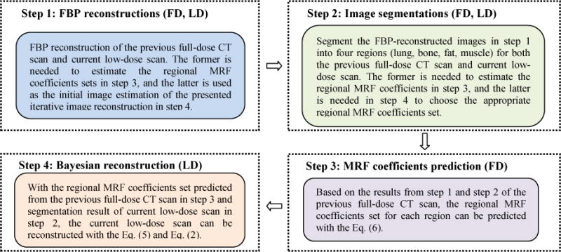
Flowchart of the proposed texture-preserving LdCT image reconstruction algorithm.

A patient, who was scheduled for CT-guided lung nodule needle biopsy at Stony Brook University Hospital, was recruited to this study under informed consent after approval by the Institutional Review Board. The patient was scanned using a Siemens CT scanner. The X-ray tube voltage was set to be 120kVp, and the tube current was set to be 100mAs for the full-dose scan. The subsequent low-dose scans were performed at 20 mAs level. The raw data were calibrated by the CT system and outputted as sinogram data or line integrals. In addition to the patient recruitment for both full- and low-dose scans, two more recruitments were made for only full-dose scans on patients, one patient has a lung nodule and the other patient has a colon polyp, both of which have a size of 10 mm.

Based on the patient scans, we first performed experiments using simulated low-dose sinogram data by adding noise to the full-dose sinogram data with the simulation tool of [6]. The reason of using simulated low-dose data is that the ground truth is available for a proof-of-concept study. Also, by a prefect registration between the full- and low-dose scans in the simulation, the region-specific MRF coefficients predicted from the neighboring slices of the full-dose image can be applied to different slices in the corresponding low-dose image reconstruction and the impact on the mismatch of slice location and, therefore the mismatch of tissue regions, can be accurately documented.

Then experiments using the acquired full- and low-dose sinogram data at 100 and 20 mAs levels from the same patient were also performed. In the 20 mAs scan, all variations, including patient movements, organ deformations, gantry positioning between the full- and low-dose scans, etc., are present. In addition, the variation associated with the image segmentation is also involved. This clinical pilot study reflects the current clinical situation.

A. Experiments on Simulated Low-dose Sinogram Data

1) Extraction of MRF Model Coefficients

Given the 100 mAs full-dose data of the patient (who has also a low-dose scan at 20 mAs level) and its simulated low-dose sinogram data, the Step 1 of Fig. 1 is to apply the well-established filtered back-projection (FBP) algorithm to reconstruct the full-dose data with Ramp filter at Nyquist frequency and the low-dose data with Hann filter at 50% Nyquist frequency. The reason of using Hann filter at 50% Nyquist frequency is because of the increased noise in the low-dose data. This smoothed FBP reconstruction of low-dose data will be treated as the initial estimate of the desired solution of Eq. (2). The full-dose FBP reconstruction will be treated as a priori image, from which the tissue image textures will be extracted.

Given the above FBP reconstructions, the Step 2 of Fig. 1 is to apply an efficient image segmentation algorithm to label the tissue regions. Because of its high computing efficiency, our previously-reported vector quantization (VQ) segmentation algorithm [31] was adopted in this exploratory study. It is fully automatic once the number of tissue types is given, e.g., setting R=4 to represent lung, bone, fat, and muscle for chest CT imaging. Moreover, we adopted morphological operations to enlarge the segmented lung parenchyma and bone region boundaries slightly so that the final lung region for MRF coefficients prediction would include both the blood vessels inside lung and the juxta-pleural nodules attached to the pleural wall. The bone marrow with relatively lower intensities was also included in the refined bone region for MRF coefficients prediction of the bone tissue. Generally, it took less than 1 second to segment a 512×512 image on a desktop computer of single CPU of 3GHz and 12 GB RAM without acceleration. Because of the high computing efficiency, the VQ algorithm was applied to the low-dose initial estimate and each refining iteration result to obtain the tissue masks. Fig. 2 illustrates an example of segmenting the full-dose image.

FIG. 2.

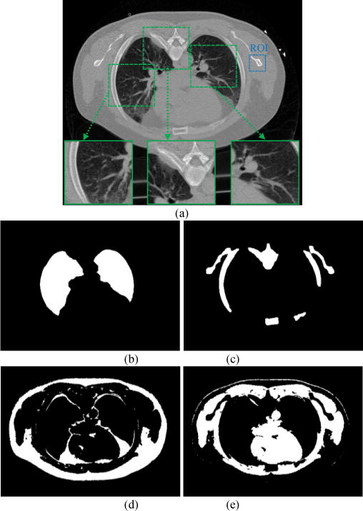
Segmented masks of the chest CT image (a). Picture (b) is the lung mask or region; (c) is the bone mask; (d) is the fat mask; and (e) is the muscle mask.

Given the segmented masks of the four tissue types from the FdCT FBP reconstruction of Fig. 2, the Step 3 of Fig. 1 is to extract the corresponding MRF model coefficients set by Eq. (6). From experiments, we found that a 7×7 MRF window size is sufficient, since the MRF coefficients beyond this window are close to zero and have nearly no impact. Fig. 3 illustrates the predicted MRF coefficients set of the four tissue regions, respectively. It is interesting to see that the MRF model coefficients of the lung and bone regions have some similarity while the coefficients of the fat and muscle regions also have some similarity, but the coefficients of the group of lung/bone are clearly different from the coefficients of the group of fat/muscle. The former group has a large intensity variation while the later group has a small intensity variation. All the four tissue regions exhibit different spectral patterns corresponding to different image textures. It is worth noting that the sum of the predicted MRF coefficients for each region, $\text{sum}({\mathbf{b}}_r^{\text{FD\_predict}})$, is close to 1, as expected.

FIG. 3.

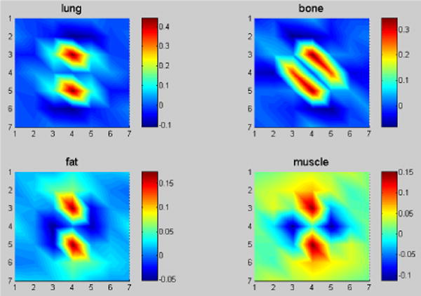
The predicted four sets of MRF model coefficients for the four tissue regions of Fig. 2 with a 7×7 MRF window size in 2D presentation. The corresponding regions are indicated by picture title.

Since our ultimate goal is to preserve these image textures of full-dose scan in the low-dose image reconstructions, the spatial mismatch between the full- and low-dose images must be considered. In the image slice (transverse) plane, the spatial mismatch is not a concern because the contents in each segmented region mask remain the same regardless where the region is located once the axial location is the same between the full- and low-dose images. Therefore, the concern would be on the mismatch of the axial location. To get insights on this, we took the slice of Fig. 3 which is located at slice #60 as the reference to investigate its nearby slices. Fig. 4 shows the predicted MRF model coefficients of the lung region from slice #58 to slice #62 of the same patient, as well as the coefficients predicted from the whole five neighboring slices. The similarity among the six sets of MRF coefficients can be quantified by the correlation coefficient measure with a value greater than 98% and with a very tiny difference (discrepancy <5%). The phenomenon of the predicted MRF model coefficients from the neighboring image slices for the lung region also holds for the other three regions (bone, fat, and muscle).

FIG. 4.

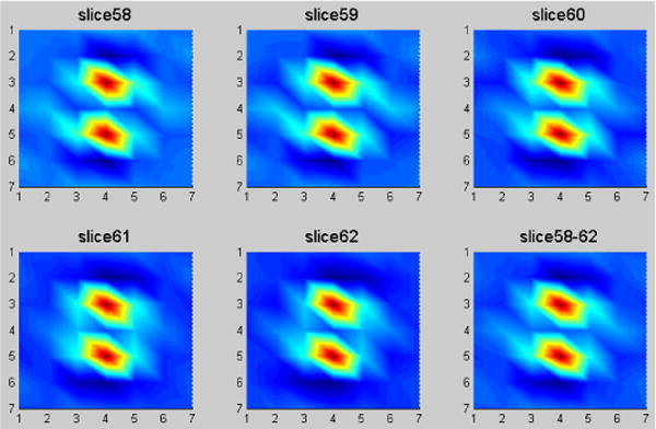
The predicted MRF coefficients of the lung region for five neighboring slices in 2D presentation. The corresponding slice numbers are indicated in picture title.

The regional spectral pattern similarity can be attributed to the tissue structure similarity among nearby image slices. Because of this similarity among nearby image slices and the region-specific nature of the estimated MRF model coefficients across the entire image slice, an accurate image alignment between the full-and low-dose in the axial direction is also not necessary. In other words, when we reconstruct one slice of the low-dose scan, we can potentially utilize the MRF model coefficients trained from the roughly-matched nearby image slices of the FdCT scan, which dramatically relieves the demand for accurate alignment of the full-dose image with the low-dose image along the axial direction and completely eliminates the need for voxel-by-voxel alignment across the transverse plane.

Given the extracted MRF model coefficients of the four major tissue regions from the full-dose image, the Step 4 of Fig. 1 is to incorporate these tissue textures into the low-dose image reconstruction. To show the gain by incorporating the textures into LdCT image reconstruction, three commonly used image reconstruction methods were implemented to set up reference for comparison purpose: (1) the FBP method; (2) the GsMRF method; (3) the HuMRF method. The comparisons were conducted by both simulated and acquired low-dose projection data experiments.

2) Image Reconstruction

From the simulated low-dose data of the patient, the sinogram of one slice (slice #60) was extracted to illustrate the first scenario of our experiments, i.e., the slice match between full- and low-dose scans. In this study, we chose β value that gave the best eye-appealing result among other values for the three MRF algorithms. The reconstructed images from the simulated low-dose sinogram by the FBP, GsMRF, HuMRF, and our proposed MRF-texture algorithm are shown in Fig. 5. It can be observed that all the MRF algorithms outperformed the FBP method in terms of noise suppression. While for the three MRF algorithms, the proposed MRF-texture is superior to both the GsMRF and the HuMRF in terms of edge/detail preservation, which will be quantified in the following sections. It should be noted that, for the MRF-texture algorithm, the region-specific MRF coefficients were predicted from the same slice of the corresponding full-dose image (i.e., slice #60, as shown in Fig. 2(a)). Therefore, we use the legend “MRF-T60” to denote the corresponding results.

FIG. 5.

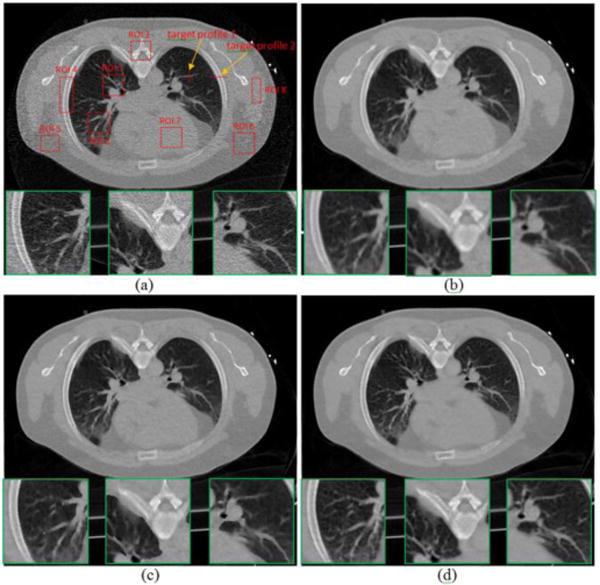
Reconstructed transverse slice of the patient from the simulated low-dose sinogram: (a) The FBP reconstruction; (b) The GsMRF reconstruction, β = 3×10⁵; (c) The HuMRF reconstruction, β = 3×10⁵, δ=0.004; and (d) The MRF-T60 reconstruction, β = 3×10⁵. All the images are displayed with the same window [0, 0.034] mm⁻¹.

According to the analysis of Fig. 3 and Fig. 4, since the predicted MRF coefficients from nearby slices show similar patterns, we may not necessarily need to utilize the MRF coefficients predicted from the exactly same slice of the corresponding FdCT scan. That is, when we reconstruct the slice #60 of the low-dose scan, we can potentially employ the MRF coefficients predicted from any one or summation of all the nearby slices (slice #58, #59, #60, #61, #62) of the full-dose scan. In this second scenario of our experiments, Fig. 6 shows the reconstructed images from the simulated low-dose sinogram data by the proposed MRF-texture algorithm using MRF coefficients predicted from different slices of the full-dose image. We can observe that the reconstructed images in Fig. 6 are very similar to each other, and the quantitative evaluations in the following sections also validate this observation.

FIG. 6.

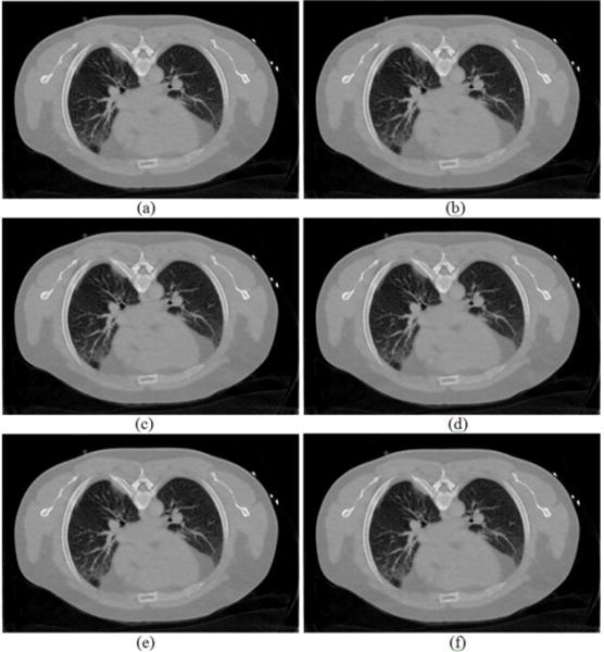
Reconstructed transverse slice of the patient by the proposed MRF-texture algorithm from the simulated low-dose sinogram: (a) The MRF-T58 reconstruction; (b) The MRF-T59 reconstruction; (c) The MRF-T60 reconstruction; (d) The MRF-T61 reconstruction; (e) The MRF-T62 reconstruction; and (f) The MRF-T58-62 reconstruction. The images were cropped for better visualization. All the images are displayed with the same window [0, 0.034] mm⁻¹.

3) Normal Vector Flow Measure

In order to quantify the texture benefit of the proposed a priori knowledge model of Eq. (5), a region of interest (ROI), indicated by a rectangular box in Fig. 2(a), was selected to plot the normal vector flow (NVF) [32] images for different reconstruction methods in Fig. 5, and the corresponding NVF images are illustrated in Fig. 7. The NVF image in Fig. 7(a) is corresponding to the FBP reconstruction from the full-dose scan of Fig. 2(a), and can serve as the reference standard. The gradual changes of the intensities in the desired image are often shown as ordered arrow in the NVF image, while the noise in the image is often shown as disordered arrows, as shown in Fig. 7(b). From Fig. 7(c)–(e), we can see that the disordered arrows in the uniform regions were suppressed by using MRF reconstruction methods. However, the ordered arrows around the bone boundaries in Fig. 7(c) swelled a little bit due to the edge blurring in the GsMRF reconstructed image of Fig. 5(b), and those in Fig. 7(d) were falsely depicted due to the brute enforcing of edge-preserving characteristics of the Huber penalty of Fig. 5(c). In contrast, the NVF image of the proposed MRF-texture algorithm in Fig. 7(e) demonstrated best matches of the ordered arrows as compared to the reference standard of Fig. 7(a), which indicates that the textures of the corresponding reconstruction were best preserved. Other quantitative measures using image quality merits, such as noise and resolution tradeoff and local image quality assessment, are reported in Appendix of this paper.

FIG. 7.

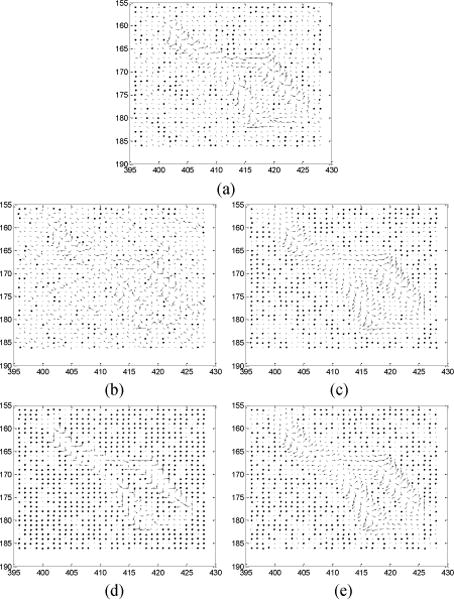
NVF images of a ROI labeled in Fig. 2(a). (a) is the reference from Fig. 2(a). (b)–(e) are corresponding to the reconstructions in Fig. 5(a)–(d).

4) Haralick Texture Measures

Haralick texture features have been widely used for classification of lesion malignancy [33] and, therefore, adopted to quantify the texture preservation in the reconstructions of the four methods above (the FBP, GsMRF, HuMRF, and MRF-texture). Eight ROIs were selected on the lung, bone, fat, and muscle, respectively, from the full-dose image in Fig. 5(a) to set up the baseline or reference. The corresponding ROIs were selected on the low-dose reconstructions of the four methods. The 14 Haralick texture measures were extracted from each ROI. The Euclidean distance between the textures of the full- and low-dose images was used as the quantitative measure. A shorter distance indicates better texture preservation by the reconstruction algorithm. Table I shows the quantitative results. The presented MRF-texture image reconstruction has the best performance on texture preservation, as expected. Because of the known textures from lung, bone, fat, and muscle from the full-dose image, the gain by the proposed MRF-texture algorithm on these four tissue types are noticeable in the low-dose image reconstruction.

TABLE I.

Texture distance between the reference full-dose image and the reconstructed low-dose images in Fig. 5.

ROI	Tissue type	FBP	GsMRF	HuMRF	MRF-T
1	lung	7.2076	2.3043	7.3989	1.7932
2	lung	6.3935	3.688	7.6508	3.5876
3	bone	8.7506	3.2533	3.1033	3.0221
4	bone	8.0978	4.3529	5.7742	3.4321
5	fat	8.8243	3.1907	2.685	2.5203
6	fat	9.3355	4.3106	3.6281	2.7702
7	muscle	9.2740	6.9097	6.9131	6.0375
8	muscle	5.7516	6.4899	5.2064	4.6562

To show how the gain on the large tissue volumes of lung, bone, fat, and muscle can lead to the gain on the texture preservation of small lung nodule or colon polyp inside the large tissue volumes, the above procedure of extracting texture information from FdCT and performing texture-preserving LdCT image reconstruction was repeated to the sinogram data of the two patients, one with a nodule and the other with a polyp, respectively. Fig. 8 shows the reconstructed images of the two patients acquired from routine protocol of full-dose level (120 kV, 100 mAs) where the ROIs were selected to compute the textures. The simulated low-dose scans were reconstructed by the four algorithms of FBP, GsMRF, HuMRF, and MRF-texture. The textures from the full-dose scans were used as the reference when comparing the texture distance of the four algorithms. Table II and Table III show the experimental outcomes. The gain from the known large tissue volumes led to a noticeable gain on the unknown small nodule or polyp.

FIG. 8.

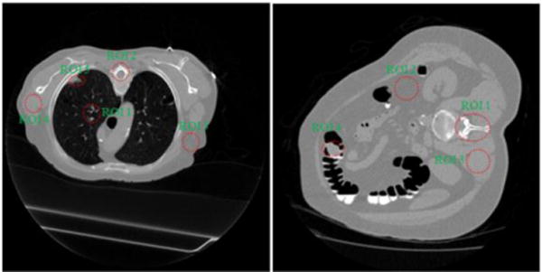
Reconstructed transverse slice of two patients from full-dose acquisitions: (a) containing a lung nodule as indicated by ROI 5; (b) containing a colonic polyp as indicated by ROI 4.

TABLE II.

Texture distance between the reference full-dose image in Fig. 8(a) and the reconstructed low-dose images by the four reconstruction algorithms.

ROI	Tissue type	FBP	GsMRF	HuMRF	MRF-T
1	lung	6.4241	5.7532	9.9530	5.0552
2	bone	8.6492	5.6968	5.9468	2.5173
3	fat	7.3578	7.4379	7.4194	6.6144
4	muscle	11.6797	3.8456	5.8283	2.8951
5	lung nodule	9.9584	4.5440	5.1329	4.3407

TABLE III.

Texture distance between the reference full-dose image in Fig. 8(b) and the reconstructed low-dose images by the four reconstruction algorithms.

ROI	Tissue type	FBP	GsMRF	HuMRF	MRF-T
1	bone	8.8206	7.8440	6.1991	4.7278
2	fat	8.9881	7.5032	6.1540	5.2425
3	muscle	8.2534	9.3631	9.2090	7.9403
4	colon polyp	9.7208	7.0602	5.8975	4.5296

B. Experiments on Real Low-dose Sinogram Data

1) Image Reconstruction

To evaluate the proposed a priori knowledge model of Eq. (5) in a more realistic situation, the real low-dose sinogram data (120 kVp, 20mAs) of the same patient (of Fig. 5) was also used to perform a pilot clinical study. The slice #45 of the low-dose scan roughly matches the slice #60 of the full-dose scan by visual judgment. Therefore, we employed the MRF coefficients sets (as shown in Fig. 3 and Fig. 4) predicted from the slice #60 and its neighboring slices of the full-dose scan to reconstruct the slice #45 of the low-dose scan.

In the first scenario of using the MRF coefficients of the slice #60, the reconstructed images from the low-dose 20mAs sinogram by the FBP, GsMRF, HuMRF and MRF-T60 methods are shown in Fig. 9. It is evident that all the three MRF methods outperformed the FBP method in terms of noise suppression, and the MRF-T60 result is superior to the GsMRF and the HuMRF in terms of edge/detail preservation.

FIG. 9.

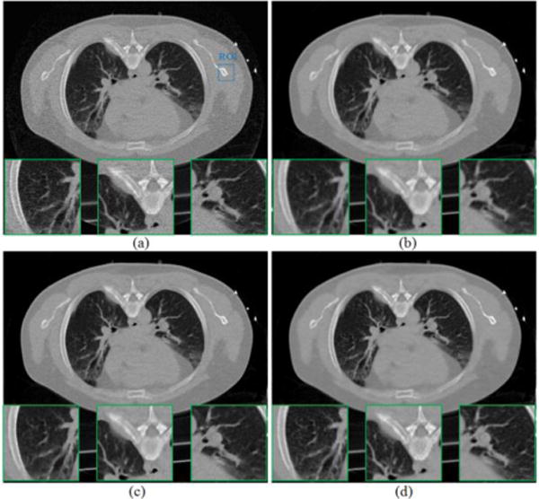
Reconstructed transverse slice of the patient data from the low-dose 20mAs sinogram: (a) The FBP reconstruction; (b) The GsMRF reconstruction, β = 1×10⁵; (c) The HuMRF reconstruction, β = 1×10⁵, δ=0.004; and (d) The MRF-T60 reconstruction, β = 1×10⁵. All the images are displayed with the same window [0, 0.034] mm⁻¹.

In the second scenario of using the MRF coefficients set of the nearby slices around the slice #60, (i.e., slice #58, #59, #60, #61, #62) of the full-dose scan to reconstruct the slice #45 of the low-dose 20mAs sinogram data, Fig. 10 shows the results of our proposed MRF-texture method. By visual judgment, the reconstructed images in Fig. 10 are very similar to each other, concurring with the simulation results of Fig. 6. Quantitative measures on the results of Fig. 9 and Fig. 10 are given below.

FIG. 10.

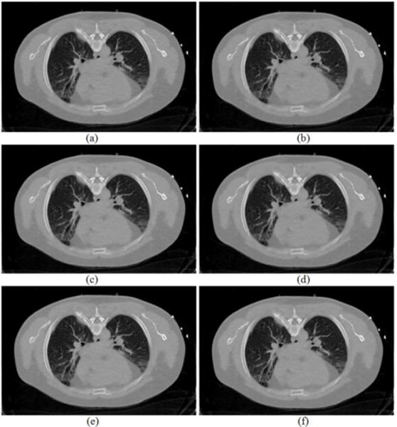
Reconstructed transverse slice of the patient by the proposed MRF-texture algorithm from the low-dose 20mAs sinogram: (a) The MRF-T58 reconstruction; (b) The MRF-T59 reconstruction; (c) The MRF-T60 reconstruction; (d) The MRF-T61 reconstruction; (e) The MRF-T62 reconstruction; and (f) The MRF-T58-62 reconstruction. All the images are displayed with the same window [0, 0.034] mm⁻¹.

2) Normal Vector Flow Study

The NVF images of a ROI as indicated in Fig. 9(a) were also plotted for the results of the four different reconstruction methods of Fig. 9, and the corresponding NVF images are illustrated in Fig. 11. The NVF image of Fig. 7(a) can be served as a reference for comparison, because that image was made from a similar ROI as that in Fig. 9(a). Despite the lacking of golden standard in this real clinical low-dose data pilot study, yet we can still observe similar phenomena as those claimed in the Section III.A of simulation study. And the NVF image of the presented MRF-texture algorithm in Fig. 11(d) has the best match to the reference in Fig. 7(a), indicating that the textures of the corresponding reconstructed image were best preserved by our proposed a priori knowledge model of Eq. (5).

FIG. 11.

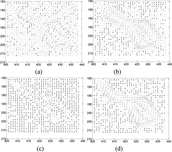
NVF images of a ROI labeled in Fig. 9(a). The NVF images in Fig. 11(a)–(d) are corresponding to the reconstructions in Fig. 9(a)–(d).

3) Evaluation by Physician Experts

In an effort to qualitatively compare the results of the four different reconstruction methods, three experienced physicians were asked to score the reconstructed images from 0 (worst) to 10 (best) in terms of noise reduction and resolution/contrast/ detail/texture preservation. The reconstructed images by different methods were displayed on the screen randomly, so it was a completely blind procedure for the physicians. Table VI lists the physicians’ scores on the reconstructed image quality under three different display windows: bone window (BW), soft tissue window (TW), and lung window (LW). It is evident that the reconstructed image by our proposed MRF-texture algorithm generally has the highest scores (with mean 7.56) and, therefore, outperformed the other three methods (with mean 3.22 for FBP, 5.67 for GsMRF, and 5.44 for HuMRF, respectively) from the physicians’ point of view.

TABLE VI.

Physicians’ scoring of the reconstructed image quality in Fig. 9 by the four reconstruction methods.

	Physician #1			Physician #2			Physician #3
	BW	TW	LW	BW	TW	LW	BW	TW	LW
FBP	3	3	2	5	4	5	3	2	2
GsMRF	7	5	4	6	5	7	5	6	6
HuMRF	5	5	5	6	5	6	7	6	4
MRF-T60	8	7	7	7	5	9	9	8	8

IV. Discussion and Conclusion

This work introduced a previous full-dose high-quality CT scan induced MRF penalty model for Bayesian image reconstruction of subsequent low-dose scans. The proposed a priori knowledge model of Eq. (5) considers the anatomical similarity among the reconstructed image series of the previous full-dose and current low-dose scans and utilizes the full-dose image to predict region-specific MRF model coefficients, which have been routinely specified by an ad hoc manner based on the nearby image voxel distance to the concerned voxel. The presented a priori knowledge model further considers the tissue specific patterns in addition to the anatomical similarity and makes the MRF model coefficients adaptive to be regionally specific, resulting in the elimination of the demand for point-by-point image registration between the full- and low-dose scans in the prediction of the model coefficients [28]. Experimental outcomes showed noticeable gain by the proposed a priori knowledge model of Eq. (5) compared to the well-known generic GsMRF penalty and HuMRF penalty (which are based on the distance model coefficients), in terms of computer-based merits and physician assessment on the reconstructed images. Essentially, the generic MRF penalty encourages regional smoothness and edge sharpness, lacking a mechanism to preserve the tissue specific characteristics or patterns (i.e., image textures). The proposed MRF-texture model takes advantages of the generic MRF penalty’s neighborhood system and also brings the a priori knowledge of the image textures into the LdCT image reconstruction. Particularly, the gain on textures of the nodule and polyp is clinically important because (1) the majority of nodules and polyps are benign and differentiation of malignant vs. benign is necessary and (2) the image textures play an important role in the lesion differentiation.

While utilizing previous full-dose image (or high-quality image) to improve the quality of follow-up LdCT images has become a research endeavor [9–16, 28], one major limitation therein is that the previous full-dose image usually needs to be registered to the current low-dose images. In practice, severe patient motion, tissue or organ deformation, fluid flow, etc. can occur between the full- and low-dose scans, where even a deformable registration may not be adequate to capture the complex anatomical and physiological motions, resulting in residual errors in the low-dose image reconstruction [15]. In our previous study of utilizing full-dose image via MRF model coefficients [28], we predicted MRF coefficients for each single voxel in the full-dose image. That is, for a 2D image with 512×512 pixels, 512×512 sets of MRF coefficients were obtained. And because of the pixel-by-pixel mechanism, accurate registration between the previous full-dose image and the current low-dose images is required before we can reconstruct the low-dose images. In contrast, the method proposed in this paper does not demand registration between the full- and low-dose scans in the transverse plane. However, it does require a segmentation step to divide each image into several tissue regions (e.g., lung, bone, fat, and muscle). And then, for a 2D image with 512×512 pixels, only 4 sets of MRF coefficients are predicted from the previous full-dose image, assuming that the pixels within the same tissue region share similar texture pattern, as shown in Fig. 3. In this study, a rough segmentation was shown to be sufficient, and the simple and fast VQ-based image segmentation approach was employed. Because of its region-by-region nature, the strategy in this work is more efficient and more feasible in practice than that of [28]. It is noted that the image in Fig. 9(a) shifts substantially compared with the image in Fig. 2(a) (the cause could be re-positioning of the patient, physiological changes like breath or heartbeat, etc.), and their detailed structures within lung region also vary substantially, but we can still utilize the region-specific MRF coefficients predicted from Fig. 2(a) to help the reconstruction of Fig. 9(a) without any registration. Along the axial direction, a rough alignment on the full- and low-dose scans is sufficient for the reconstruction of the low-dose scans by the presented MRF-texture algorithm. This statement is based on the results in Fig. 6 and Fig. 10, which use nearby slice-predicted MRF coefficients, and the outcomes were very satisfactory.

In this proof-of-concept study, we used 2D MRF window (with size 7×7) when computing the MRF model coefficients and reconstructing each transverse image, while the 3D volume was formed as a stack of 2D transverse images. Although lacking of regularization in axial direction, we did not observe artifacts in the coronal or sagittal views of the reconstructed volume. However, a 3D MRF window (e.g., with size 7×7×3), which results in fully 3D MRF-texture regularization, may be beneficial and would be investigated in our future study.

The smoothing parameter β in Eq. (2) controls the tradeoff between the data fidelity term and the penalty term. A larger β value produces a more smoothed reconstructed image with lower noise level but also lower resolution, and vice versa. Determining the optimal β value for SIR methods is still an open question. In this study, we chose β value that gave the best eye-appealing result among other values for the three MRF algorithms. For the presented MRF-texture algorithm, we observed that, as long as the β in a reasonable range (within an order of magnitude) around the optimal value, the image texture does not change noticeably. That is, the desired texture does not require extremely careful tuning of β.

Shared with other iterative reconstruction methods, the proposed MRF-texture algorithm is iterative and demands intensive computing power to perform the multiple re-projection and back-projection operation cycles in the projection and image domains, although the image segmentation and MRF coefficients prediction steps are pretty fast. Fast computer with GPU-assisted implementation is expected to dramatically accelerate the associated computation for possible clinical practice. It is also noted that because of limited clinical datasets, further evaluation using more real patient datasets and specific clinical tasks is necessary to show the clinical significance and, therefore, is under progress.

Appendix: Image Quality Evaluation

1) Noise and Resolution Tradeoff

In addition to the above NVF and Haralick texture related measures on the reconstruction results of Fig. 5, we further evaluated the results in terms of noise reduction and resolution preservation. As noted above that the parameter β of the three MRF algorithms controls the noise and resolution tradeoff, which means one can always sacrifice spatial resolution for better noise performance by increasing the value of β, or vice versa. In this study, we selected the β value for the three MRF algorithms to have similar noise level at uniform regions. The noise level of the reconstructed images was quantified by the standard deviation of the four uniform ROIs (ROI 5–ROI 8) shown in Fig. 5(a). The image resolution can be characterized by a vertical and a horizontal profile labeled by the red lines in Fig. 5(a). Fig. 12 compares the profiles. The comparison demonstrated the advantage of the presented MRF-texture algorithm over the GsMRF and HuMRF on edge and contrast preservation.

FIG. 12.

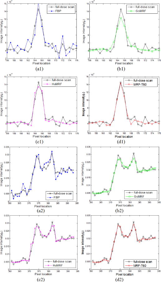
Comparison of the profiles along the vertical line and the horizontal line labeled in Fig. 5(a) between the four reconstruction methods with simulated low-dose sinogram and the FBP reconstruction with the full-dose sinogram.

As reported above, the MRF coefficients from nearby image slices are very similar and the resulting images by the MRF-texture algorithm are also very similar in terms of noise reduction and resolution preservation, as shown in Fig. 6. To visualize the similarity, profiles were drawn from the images in Fig. 6 and are shown by Fig. 13, which demonstrates that the profiles of the reconstructed images in Fig. 6 are nearly overlapped with each other. The similarity reveals that the proposed MRF-texture algorithm using MRF coefficients predicted from nearby slices of the previous full-dose image can generally produce very similar reconstruction results.

FIG. 13.

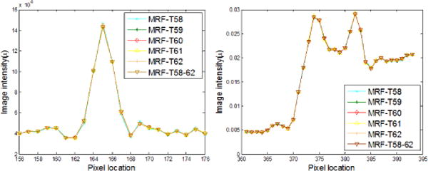
Comparison of the profiles along the vertical line and the horizontal line labeled in Fig. 5(a) for the proposed MRF-texture algorithm using different MRF coefficients sets with simulated low-dose sinogram.

2) Local Image Quality Assessment

To further quantitatively demonstrate the benefits of our proposed a priori knowledge model of Eq. (5), we compared the reconstruction results of Fig. 5 on the ROIs, which have detailed structures (ROI 1 – ROI 4) and were labeled with red rectangles in Fig. 5(a). Two quantitative metrics were used to evaluate the image quality of the ROIs. The first metric is the traditional root mean squared error (RMSE), which indicates the difference between the reconstructed image and the reference image, and characterizes the reconstruction accuracy. The second metric is the universal quality index (UQI) [34] which measures the similarity between the reconstructed image and the ground truth image, and quantifies the noise, spatial resolution, and texture correlation between two images.

The corresponding quantitative results with the two metrics are shown in Fig. 14. As we can see, the proposed MRF-texture algorithm offered the lowest RMSE and the highest UQI for all the four detailed ROIs. As expected that the three MRF algorithms would perform better than the FBP method.

FIG. 14.

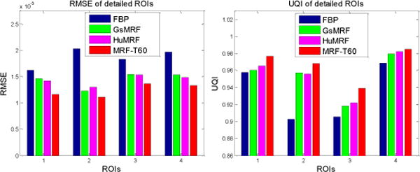
Performance comparison of the four reconstruction methods on their reconstructions’ ROIs labeled in Fig. 5(b) with RMSE and UQI metrics. The corresponding reconstruction methods are illustrated in figure legend.

The image quality similarity of the reconstructed ROIs in Fig. 6 was also evaluated with the RMSE and UQI metrics, and the corresponding results are shown in Fig. 15. It can be seen that all the reconstructions’ ROIs in Fig. 6 by different MRF coefficients sets are close to each other. These local image quality assessments can also conclude that the proposed MRF-texture algorithm using MRF coefficients predicted from the nearby slices of the previous full-dose image can generate very similar reconstructed images at low-dose levels.

FIG. 15.

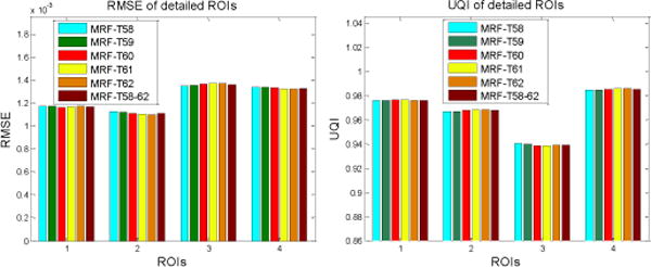
Performance comparison of the proposed MRF-texture algorithm using different MRF coefficient sets on the reconstruction of the detailed ROIs labeled in Fig. 5(a) with RMSE and UQI metrics. The corresponding MRF coefficient sets are illustrated in figure legend.

References

- 1.Brenner D, Hall E. CT – An increasing source of radiation exposure. The New England Journal of Medicine. 2007;357:2277–2284. doi: 10.1056/NEJMra072149. [DOI] [PubMed] [Google Scholar]
- 2.Kalender W. Dose in X-ray CT. Physics in Medicine and Biology. 2014;59:R129–R150. doi: 10.1088/0031-9155/59/3/R129. [DOI] [PubMed] [Google Scholar]
- 3.Haaga J, Alfidi R. Precise biopsy localisation by CT. Radiology. 1976;118:603–607. doi: 10.1148/118.3.603. [DOI] [PubMed] [Google Scholar]
- 4.Tacelli N, Remy-Jardin M, Copin M, et al. Assessment of non-small cell lung cancer perfusion: Pathologic-CT correlation in 15 patients. Radiology. 2010;257:863–872. doi: 10.1148/radiol.10100181. [DOI] [PubMed] [Google Scholar]
- 5.Liang Z, Lu H, Li X. Noise treatment of low-dose CT projections and images. 7,187,794 B2. US Patent Number. (filed in 2002 and approved in 2007)
- 6.Wang J, Li T, Lu H, Liang Z. Penalized weighted least-squares approach to sinogram noise reduction and image reconstruction for low-dose X-ray CT. IEEE Transactions on Medical Imaging. 2006;25:1272–1283. doi: 10.1109/42.896783. [DOI] [PMC free article] [PubMed] [Google Scholar]
- 7.Fessler J. Statistical image reconstruction methods for transmission tomography. Handbook of Medical Imaging. 2000;2:1–70. [Google Scholar]
- 8.Thibault JB, Sauer K, Bouman C, Hsieh J. A three-dimensional statistical approach to improved image quality for multislice helical CT. Med Phys. 2007;34:4526–4544. doi: 10.1118/1.2789499. [DOI] [PubMed] [Google Scholar]
- 9.Nett B, Tang J, Aagaard-Kienitz B, Rowley H, Chen G. Low radiation dose C-arm cone-beam CT based on prior image constrained compressed sensing (PICCS): Including compensation for image volume mismatch between multiple data acquisitions. Proc SPIE Medical Imaging. 2009;7258:725–803. [Google Scholar]
- 10.Yu H, Zhao S, Hoffman E, Wang G. Ultra-low dose lung CT perfusion regularized by a previous scan. Academic Radiology. 2009;16:363–373. doi: 10.1016/j.acra.2008.09.003. [DOI] [PMC free article] [PubMed] [Google Scholar]
- 11.Ma J, Huang J, Feng Q, Zhang H, Lu H, Liang Z, Chen W. Low-dose CT image restoration using previous normal-dose scan. Medical Physics. 2011;38:5713–5731. doi: 10.1118/1.3638125. [DOI] [PMC free article] [PubMed] [Google Scholar]
- 12.Ouyang L, Solberg T, Wang J. Noise reduction in low-dose cone beam CT by incorporating prior volumetric image information. Medical Physics. 2012;39:2569–2577. doi: 10.1118/1.3702592. [DOI] [PubMed] [Google Scholar]
- 13.Lee H, Xing L, Davidi R, Li R, Qian J, Lee R. Improved compressed sensing-based cone-beam CT reconstruction using adaptive prior image constraints. Physics in Medicine and Biology. 2012;57(8):2287–2307. doi: 10.1088/0031-9155/57/8/2287. [DOI] [PubMed] [Google Scholar]
- 14.Stayman J, Dang H, Ding Y, Siewerdsen J. PIRPLE: A penalized-likelihood framework for incorporation of prior images in CT reconstruction. Physics in Medicine and Biology. 2013;58(21):7563–7582. doi: 10.1088/0031-9155/58/21/7563. [DOI] [PMC free article] [PubMed] [Google Scholar]
- 15.Dang H, Wang A, Sussman M, Siewerdsen J, Stayman J. dPIRPLE: A joint estimation framework for deformable registration and penalized likelihood CT image reconstruction using prior images. Physics in Medicine and Biology. 2014;59:4799–4826. doi: 10.1088/0031-9155/59/17/4799. [DOI] [PMC free article] [PubMed] [Google Scholar]
- 16.Zhang H, Huang J, Ma J, Bian Z, Feng Q, Lu H, Liang Z, Chen W. Iterative reconstruction for X-ray CT using prior-image induced nonlocal regularization. IEEE Transactions on Biomedical Engineering. 2014;61(9):2367–2378. doi: 10.1109/TBME.2013.2287244. [DOI] [PMC free article] [PubMed] [Google Scholar]
- 17.Chen G, Tang J, Leng S. Prior image constrained compressed sensing (PICCS): A method to accurately reconstruct dynamic CT images from highly undersampled projection data sets. Medical Physics. 2008;35:660–663. doi: 10.1118/1.2836423. [DOI] [PMC free article] [PubMed] [Google Scholar]
- 18.Ng F, Ganeshan B, Kozarski R, et al. Assessment of primary CRC heterogeneity by using whole-tumor texture analysis. Radiology. 2013;266(1):177–184. doi: 10.1148/radiol.12120254. [DOI] [PubMed] [Google Scholar]
- 19.Aerts H, Velazquez E, Leijenaar R, et al. Decoding tumour phenotype by noninvasive imaging using a quantitative radiomics approach. Nature Communications. 2014;5:1–8. doi: 10.1038/ncomms5006. [DOI] [PMC free article] [PubMed] [Google Scholar]
- 20.McCollough CH, Yu L, Kofler JM, Leng S, Zhang Y, Li Z, Cater RE. Degradation of CT low-contrast spatial resolution due to the use of iterative reconstruction and reduced dose levels. Radiology. 2015;276(2):499–506. doi: 10.1148/radiol.15142047. [DOI] [PMC free article] [PubMed] [Google Scholar]
- 21.Bian J, Yang K, Boone J, Han X, Sidky E, Pan X. Investigation of iterative image reconstruction in low-dose breast CT. Physics in Medicine and Biology. 2014;59(11):2659–2685. doi: 10.1088/0031-9155/59/11/2659. [DOI] [PMC free article] [PubMed] [Google Scholar]
- 22.Kim H, Chung Y, Lee Y, Choi J, Park M, Kim M, Kim K. Quantitative analysis of the effect of iterative reconstruction using a phantom: determining the appropriate blending percentage. Yonsei Medical Journal. 2015;56(1):253–261. doi: 10.3349/ymj.2015.56.1.253. [DOI] [PMC free article] [PubMed] [Google Scholar]
- 23.Geman S, Geman D. Stochastic relaxation, Gibbs distributions, and the Bayesian restoration of images. IEEE Transactions on Pattern Analysis and Machine Intelligence. 1984;6:721–741. doi: 10.1109/tpami.1984.4767596. [DOI] [PubMed] [Google Scholar]
- 24.Li T, Li X, Wang J, Wen J, Lu H, Hsieh J, Liang Z. Nonlinear sinogram smoothing for low-dose X-ray CT. IEEE Transactions on Nuclear Science. 2004;51:2505–2513. [Google Scholar]
- 25.Wang J, Lu H, Eremina D, Zhang G, Wang S, Chen J, Manzione J, Liang Z. An experimental study on the noise properties of X-ray CT sinogram data in the Radon space. Physics in Medicine and Biology. 2008;53:3327–3341. doi: 10.1088/0031-9155/53/12/018. [DOI] [PMC free article] [PubMed] [Google Scholar]
- 26.Ma J, Liang Z, Fan Y, Liu Y, Huang J, Chen W, Lu H. Variance analysis of X-ray CT sinograms in the presence of electronic noise background. Medical Physics. 2012;39:4051–4065. doi: 10.1118/1.4722751. [DOI] [PMC free article] [PubMed] [Google Scholar]
- 27.Wang J, Sauer K, Thibault J, Yu Z, Bouman C. Prediction coefficients estimation in Markov random field for iterative X-ray CT reconstruction. Proc SPIE Medical Imaging. 2012;8314:831444-1–831444-9. [Google Scholar]
- 28.Zhang H, Han H, Wang J, Ma J, Liu Y, Moore W, Liang Z. Deriving adaptive MRF coefficients from previous normal-dose CT scan for low-dose image reconstruction via penalized weighted least-squares minimization. Medical Physics. 2014;41(4):041916-1–15. doi: 10.1118/1.4869160. [DOI] [PMC free article] [PubMed] [Google Scholar]
- 29.Draper N, Smith H. Applied Regression Analysis. Third. Wiley; 1998. [Google Scholar]
- 30.Han H. PhD Dissertation. State University of New York; Stony Brook: 2011. Least sine squares and robust compound regression analysis. [Google Scholar]
- 31.Han H, Li L, Han F, Song B, Moore W, Liang Z. Fast and adaptive detection of pulmonary nodules in thoracic CT images using a hierarchical vector quantization scheme. IEEE Journal of Biomedical and Health Informatics. 2015;19(2):648–659. doi: 10.1109/JBHI.2014.2328870. [DOI] [PMC free article] [PubMed] [Google Scholar]
- 32.Liu Y, Liang Z, Ma J, Lu H, Wang K, Zhang H, Moore W. Total variation-stokes strategy for sparse-view X-ray CT image reconstruction. IEEE Transactions on Medical Imaging. 2014;33:749–763. doi: 10.1109/TMI.2013.2295738. [DOI] [PMC free article] [PubMed] [Google Scholar]
- 33.Haralick R, Shanmugam K, Dinstein I. Textural features for image classification. IEEE Transactions on Systems, Man and Cybernetics. 1973;3(6):610–621. [Google Scholar]
- 34.Wang Z, Bovik A. A universal image quality index. IEEE Signal Process Letter. 2002;9:81–84. [Google Scholar]