SITDEM: A simulation tool for disease/endpoint models of association studies based on single nucleotide polymorphism genotypes

Abstract

The association analysis between single nucleotide polymorphisms (SNPs) and disease or endpoint in genome-wide association studies (GWAS) has been considered as a powerful strategy for investigating genetic susceptibility and for identifying significant biomarkers. The statistical analysis approaches with simulated data have been widely used to review experimental designs and performance measurements. In recent years, a number of authors have proposed methods for the simulation of biological data in the genomic field. However, these methods use large-scale genomic data as a reference to simulate experiments, which may limit the use of the methods in the case where the data in specific studies are not available. Few methods use experimental results or observed parameters for simulation. The goal of this study is to develop a Web application called SITDEM to simulate disease/endpoint models in three different approaches based on only parameters observed in GWAS. In our simulation, a key task is to compute the probability of genotypes. Based on that, we randomly sample simulation data. Simulation results are shown as a function of p-value against odds ratio or relative risk of a SNP in dominant and recessive models. Our simulation results show the potential of SITDEM for simulating genotype data. SITDEM could be particularly useful for investigating the relationship among observed parameters for target SNPs and for estimating the number of variables (SNPs) required to result in significant p-values in multiple comparisons. The proposed simulation tool is freely available at http://www.snpmodel.com.

1. Background

A single nucleotide polymorphism (SNP) is one of the common types of genetic variation among humans [1]. The prevalence of single nucleotide variation in the genome is about 1% [2]. Genome-wide association studies (GWAS) have identified many susceptibility SNPs that show the evidence of association with common complex diseases or treatment outcomes [3–6]. As of April 2013, an online catalog of GWAS contained nearly 1600 publications and 9900 SNPs that have associations with 1750 traits and diseases [4,7].

To identify disease phenotypes, disease models are commonly employed, using a genotype coding strategy. For example, genotypes AA, AB, and BB are coded as 0, 1, and 2, where a dominant model is coded as 0 for AA and 2 for BB and AB while a recessive model is coded as 2 for BB and 0 for AA and AB, assuming that B is the less frequent allele [8]. In GWAS, the odds ratio and relative risk are widely used to evaluate the significance of risk effect in dominant and recessive models [9,10]. In other words, the effect of a specific genotype at a SNP on the association with disease susceptibility can be approximately estimated by assessing the odds ratio or relative risk [11].

There have been many efforts to develop simulation approaches for genotype data analysis. Su et al. proposed a resampling algorithm, HAPGEN2, to simulate case–control multiple SNPs on a single chromosome [12]. GWAsimulator was designed to improve the speed of sampling whole-genome genotype data, using a rapid moving-window algorithm [13]. These simulators require existing HapMap data as a reference panel to generate simulated data. Terwilliger et al. simulated large-scale genomic data with a disease prevalence, risk allele frequency, and penetrance ratios [14]. His group has designed several freely available software packages including simQTL and DETECTANCE for genetic epidemiology studies (http://linkage.cpmc.columbia.edu/). National Cancer Institute (NCI) provides Genetic Simulation Resources (GSR) consisting of several available software tools for genetic research (http://popmodels.cancercontrol.cancer.gov/gsr/). A number of useful software packages including Haploview [15] and PLINK [16] have been developed to help analyze and visualize genetic data. Haploview is a widely used application designed to expedite the computation of linkage disequilibrium. PLINK provides useful tools to efficiently process large-scale data in whole-genome association studies. However, all the simulators introduced above simulate large regions in GWAS requiring a reference dataset and lack the ability to statistically estimate a single SNP identified in a given cohort. For example, when we have an odds ratio and its p-value for a SNP in GWAS analysis, we are able to know only the absolute importance of the SNP from the two parameters. However, the relative importance of the SNP (the extent of significance of the observed odds ratio and p-value at all possible ranges that can be obtained by the combination of other parameters of the SNP) is unclear. To address this issue, we propose new simulation methods that investigate the possible range of p-value and odds ratio (or relative risk) of a single SNP given observed parameters without using HapMap data. We introduce three simulation approaches for dominant and recessive models. Each simulation type uses different parameters, including odds ratio, relative risk, penetrance values, and the prevalence of endpoint in the population. As a result of the simulation, we are able to find the relationship among these parameters and p-values against corresponding odds ratios or relative risks.

2. Implementation

For a single genetic locus with two alleles (referred to as A and B in this study), three genotypes are possible: AA, AB, and BB. Suppose that A and B represent the major and minor frequency allele at each locus, respectively [17]. That is, of the two alleles at a SNP, an allele with the less frequency of occurrence in a cohort becomes B. For a one-locus diallelic disease model using odds ratio (or relative risk) as a measure of association between a SNP and disease risk, commonly used approaches are dominant (AA vs. AB+BB) and recessive (AA+AB vs. BB) models [18]. In this study, we propose three methods for simulation of disease/endpoint models for which each simulation type uses different parameters.

3. Simulation type I

In this simulation type, we suppose that a minor allele frequency (MAF; denoted by α) and penetrance values are known. Using these parameters, we compute the probability for genotypes based on which simulated data in each group [endpoint (N) and non-endpoint (NE)] are randomly sampled. Suppose that p(E|BB), p(E|AB), and p(E|AA) indicate the probabilities of endpoint given genotypes BB, AB, and AA, respectively. Let f_BB, f_AB, and f_AA denote the penetrance values for genotypes BB, AB, and AA, respectively. If Hardy–Weinberg equilibrium (HWE) conditions hold (i.e., p(BB)=α², p(AB)=2α(1−α), and p(AA)=(1−α)²), we can express the prevalence of endpoint in the population as follows:

$$\begin{array}{l}K=p\left(E\right)=p\left(E|BB\right)p\left(\mathit{BB}\right)+p\left(E|AB\right)p\left(\mathit{AB}\right)+p\left(E|AA\right)p\left(\mathit{AA}\right)\\ ={\alpha }^2\times f_{\mathit{BB}}+2\alpha \left(1-\alpha \right)\times f_{\mathit{AB}}+{\left(1-\alpha \right)}^2\times f_{\mathit{AA}}.\end{array}$$ (1)

Using Bayes’s theorem, given an endpoint, the probabilities of BB, AB, and AA that are denoted by p_BB, p_AB, and p_AA can be computed as follows:

$$\begin{array}{l}{p}_{\mathit{BB}}=p\left(BB|E\right)=p\left(E|BB\right)p\left(\mathit{BB}\right)/p\left(E\right)={\alpha }^2\times f_{\mathit{BB}}/K,\\ p_{\mathit{AB}}=p\left(AB|E\right)=p\left(E|AB\right)p\left(\mathit{AB}\right)/p\left(E\right)=2\alpha \left(1-\alpha \right)\times f_{\mathit{AB}}/K,\\ p_{\mathit{AA}}=p\left(AA|E\right)=p\left(E|AA\right)p\left(\mathit{AA}\right)/p\left(E\right)={\left(1-\alpha \right)}^2\times f_{\mathit{AA}}/K.\end{array}$$ (2)

Likewise, the prevalence of non-endpoint in the population is defined by the following:

$$p\left(NE\right)=1-p\left(E\right)=1-K.$$ (3)

Given a non-endpoint, the probabilities of BB, AB, and AA that are denoted by q_BB, q_AB, and q_AA are expressed as follows:

$$\begin{array}{l}{q}_{\mathit{BB}}=p\left(BB|NE\right)=p\left(NE|B\right)p\left(\mathit{BB}\right)/p\left(NE\right)={\alpha }^2\times \left(1-f_{\mathit{BB}}\right)/\left(1-K\right),\\ q_{\mathit{AB}}=p\left(AB|NE\right)=p\left(NE|B\right)p\left(\mathit{AB}\right)/p\left(NE\right)=2\alpha \left(1-\alpha \right)\times \left(1-f_{\mathit{AB}}\right)/\left(1-K\right),\\ q_{\mathit{AA}}=p\left(AA|E\right)=p\left(NE|AA\right)p\left(\mathit{AA}\right)/p\left(NE\right)={\left(1-\alpha \right)}^2\times \left(1-f_{\mathit{AA}}\right)/\left(1-K\right).\end{array}$$ (4)

Table 1 shows a probability table that summarizes all probabilities computed above for the simulation of endpoint models. Based on Table 1, p_AA, p_BB+AB=p_BB+p_AB, q_AA, and q_BB+AB=q_BB+q_AB are used for the dominant model, and p_BB, p_AB+AA=p_AB+p_AA=q_BB, and q_AB+AA=q_AB+q_AA are used for the recessive model. After the probabilities of genotypes are determined, random samples are generated using a random sampling function (e.g., “randsample” in MATLAB). That is, the number of patients who have or do not have the given genotypes is randomized based on the probabilities of the genotypes. No other factors are randomized. Let N(p_AA) and N (p_BB+AB) denote the number of patients who have and do not have a genotype AA, respectively, in a disease group. For example, suppose that we have p_AA=0.6, p_BB+AB=0.4, and the number of patients who have disease=200. We perform “R=randsample(0:1, 200, true, [0.6 0.4])” in MATLAB and count the number of 0’s and 1’s from the output R that will be N(p_AA) and N(p_BB+AB), respectively. Likewise, N(q_AA) and N(q_BB+AB) are determined. Then, an odds ratio (relative risk) and its p-value are calculated. This procedure is repeated many times.

Table 1.

A probability table for simulation of endpoint models.

	BB	AB	AA
Endpoint	pBB=α2×fBB/K	pAB=2α(1−α)×fAB/K	pAA=(1−α)2×fAA/K
Non-endpoint	qBB=α2×(1−fBB)/(1−K)	qAB=2α(1−α)×(1−fAB)/(1−K)	qAA=(1−α)2×(1−fAA)/(1−K)
HWEa	p(BB)=α2	p(AB)=2α(1−α)	p(AA)=(1−α)2

^aHWE=Hardy–Weinberg equilibrium.

In the procedure to make the probability table, Simulation type I that uses Bayes’s theorem is completely different from Simulation types II and III that will be introduced in the following subsections. The difference between Simulation types II and III is that Simulation type II uses odds ratio whereas Simulation type III uses relative risk as a simulation parameter. Therefore, Simulation types II and III have similar deployment of equations.

4. Simulation type II

In this simulation type, it is assumed that an MAF, the prevalence of endpoint (K), and an odds ratio (r) are given for simulation. For dominant and recessive models, the probabilities shown in Table 1 are computed differently.

4.1. Dominant model

By definition of odds ratio in the dominant model, we have

$$r=\frac{q_{\mathit{AA}}\left(p_{\mathit{BB}}+p_{\mathit{AB}}\right)}{p_{\mathit{AA}}\left(q_{\mathit{BB}}+q_{\mathit{AB}}\right)}=\frac{q_{\mathit{AA}}\left(1-p_{\mathit{AA}}\right)}{p_{\mathit{AA}}\left(1-q_{\mathit{AA}}\right)}.$$ (5)

Therefore, q_AA can be expressed as follows:

$$q_{\mathit{AA}}=\frac{r{p}_{\mathit{AA}}}{1-p_{\mathit{AA}}+r{p}_{\mathit{AA}}}.$$ (6)

By Hardy–Weinberg equilibrium, we know

$$p_{\mathit{AA}}K+q_{\mathit{AA}}\left(1-K\right)={\left(1-\alpha \right)}^2$$ (7)

Substituting Eq. (6) into Eq. (7), we have

$${p_{\mathit{AA}}}^{2}K\left(r-1\right)+p_{\mathit{AA}}\left(r\left(1-K\right)+K-\left(r-1\right){\left(1-\alpha \right)}^2\right)-{\left(1-\alpha \right)}^2=0.$$

Solving this equation, p_AA becomes

$$p_{\mathit{AA}}=\{\begin{array}{ll}{\left(1-\alpha \right)}^2& \text{if}r=1\\ \frac{-b\pm \sqrt{b^2+4K\left(r-1\right){\left(1-\alpha \right)}^2}}{2K\left(r-1\right)}& \text{otherwise}\end{array},$$ (8)

where

$$b=r-\left(r-1\right)\left({\left(1-\alpha \right)}^2+K\right).$$

Substituting Eq. (8) into Eq. (6), we obtain q_AA.

Now we have all four probabilities (p_AA, p_BB+AB=1−p_AA, q_AA, and q_BB+AB=1−q_AA) for random sampling.

4.2. Recessive model

Similarly, the odds ratio in the recessive model is defined as follows:

$$r=\frac{p_{\mathit{BB}}\left(q_{\mathit{AB}}+q_{\mathit{AA}}\right)}{q_{\mathit{BB}}\left(p_{\mathit{AB}}+p_{\mathit{AA}}\right)}=\frac{p_{\mathit{BB}}\left(1-q_{\mathit{BB}}\right)}{q_{\mathit{BB}}\left(1-p_{\mathit{BB}}\right)}.$$ (9)

By Hardy–Weinberg equilibrium, the following equation is held:

$$p_{\mathit{BB}}K+q_{\mathit{BB}}\left(1-K\right)={\alpha }^2.$$ (10)

Then, using Eqs. (9) and (10), we can obtain p_BB:

$$p_{\mathit{BB}}=\{\begin{array}{ll}{\alpha }^2& \text{if}r=1\\ \frac{-b\pm \sqrt{b^2-4Kr\left(r-1\right){\alpha }^2}}{2K\left(r-1\right)}& \text{otherwise}\end{array},$$ (11)

where

$$b=\left(1-r\right)\left({\alpha }^2+K\right)-1.$$

Similar to the dominant model, we can compute the remaining probabilities: p_AB+AA=1−p_BB, q_BB, and q_AB+AA=1−q_BB.

5. Simulation type III

In this simulation type, a relative risk ( $\stackrel{\sim }{r}$) is employed instead of the odds ratio used in the simulation type II. There is a tendency that the odds ratio overestimates the relative risk when the odds ratio is larger than 1 [19,20]. This overestimation becomes larger when the number of incidences of outcome increases. When the odds ratio is less than 1, it underestimates the relative risk. The relative risk is more interpretable whereas one advantage of the odds ratio is that it is not dependent on the event’s occurrence or failure. Therefore, it may be useful to calculate both measures to cross-check results [21].

5.1. Dominant model

By definition of relative risk in the dominant model, we have

$$\begin{array}{l}\stackrel{\sim }{r}=\frac{(p_{\mathit{BB}}+p_{\mathit{AB}})}{K(p_{\mathit{AA}}K+q_{\mathit{AA}}(1-K\left)\right)p_{\mathit{AA}}K\left(\right(p_{\mathit{BB}}+p_{\mathit{AB}})K+(q_{\mathit{BB}}+q_{\mathit{AB}}\left)\right(1-K\left)\right)}\\ =\frac{(1-p_{\mathit{AA}})(p_{\mathit{AA}}K+q_{\mathit{AA}}(1-K\left)\right)}{p_{\mathit{AA}}\left(\right(1-p_{\mathit{AA}})K+(1-q_{\mathit{AA}}\left)\right(1-K\left)\right)}.\end{array}$$ (12)

Using Eqs. (7) and (12), we obtain

$$p_{\mathit{AA}}=\frac{{\left(1-\alpha \right)}^2}{\stackrel{\sim }{r}\left(2\alpha -{\alpha }^2\right)+{\left(1-\alpha \right)}^2}.$$ (13)

Substituting Eq. (13) into Eq. (7), we compute q_AA. Accordingly, we can obtain p_BB+AB=1−p_AA and q_BB+AB=1−q_AA.

5.2. Recessive model

Similarly, the relative risk in the recessive model is expressed as follows:

$$\begin{array}{l}\stackrel{\sim }{r}=\frac{p_{\mathit{BB}}K\left(\right(p_{\mathit{AB}}+p_{\mathit{AA}})K+(q_{\mathit{AB}}+q_{\mathit{AA}}\left)\right(1-K\left)\right)}{(p_{\mathit{AB}}+p_{\mathit{AA}})K(p_{\mathit{BB}}K+q_{\mathit{BB}}(1-K\left)\right)}\\ =\frac{p_{\mathit{BB}}\left(\right(1-p_{\mathit{BB}})K+(1-q_{\mathit{BB}}\left)\right(1-K\left)\right)}{(1-p_{\mathit{BB}})(p_{\mathit{BB}}K+q_{\mathit{BB}}(1-K\left)\right)}.\end{array}$$ (14)

Using Eqs. (10) and (14), p_BB becomes

$$p_{\mathit{BB}}=\frac{\stackrel{\sim }{r}{\alpha }^2}{1+{\alpha }^2\left(\stackrel{\sim }{r}-1\right)}.$$ (15)

Substituting Eq. (15) into Eq. (10), we can obtain q_BB. Finally, we have all four probabilities: p_BB, p_AB+AA=1−p_BB, q_BB, and q_AB+AA=1−q_BB.

6. Results

We tested the proposed simulation methods for disease/endpoint models based on SNP genotypes. Fig. 1 shows a screenshot of simulation results using SITDEM. Fig. 2 illustrates an example of experimental results obtained using the simulation type III. In this test, the following parameters were used: $\stackrel{\sim }{r}=1.3$, K=0.3, and 200 samples. To investigate the change of p-value against predicted relative risk according to the MAF, the experiment was iterated with different MAF values (α=0.1, 0.2, 0.3). After 10,000 simulations, −log₁₀(p-values) were averaged in each bin (the size of bin=0.2) of the predicted relative risk. In this study, Fisher’s exact test was employed to compute the p-value. It was observed that as the MAF increased, the −log₁₀(p-value) also increased in both dominant and recessive models. It is worthy of noting that the −log₁₀(p-value) in the dominant model was greater than that in the recessive model. The dominant model had a smaller standard deviation when α=0.2 and 0.3. In contrast, when α=0.1, the recessive model had a smaller standard deviation.

Fig. 1.

A screenshot of simulation results in SITDEM. The following parameters were used: minor allele frequency=0.3, rate of endpoint=0.3, odds ratio=1.6, the number of samples=1000, and the number of simulations=5000.

Fig. 2.

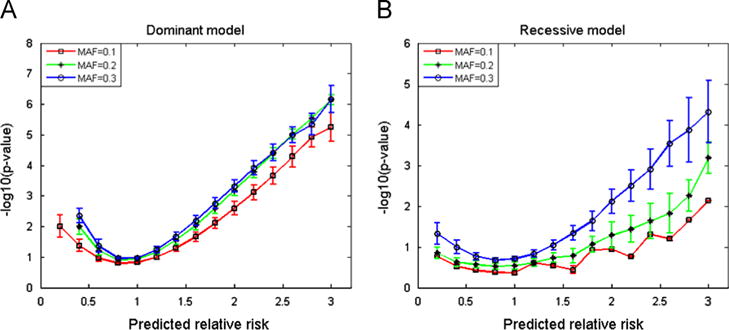
Experimental results for different minor allele frequencies in the simulation type III. This plot shows the −log₁₀(p-value) against predicted relative risk in (A) dominant and (B) recessive models.

We also simulated a special case with an odds ratio of 1. With α=0.3, 300 samples, and different prevalences of endpoint (K=0.05, 0.15, 0.3, 0.5, 0.7, 0.85, 0.95), dominant and recessive models were tested. Fig. 3(A) and (B) illustrates the −log₁₀(p-value) against predicted odds ratio in the dominant and recessive models, respectively, after 10,000 simulations. As shown in the figure, when K=0.5 (i.e., when the number of cases and controls is the same), the largest −log₁₀(p-values) were obtained in both models. The −log₁₀(p-value) was greater in the dominant model than in the recessive model.

Fig. 3.

Simulation results with minor allele frequency=0.3, odds ratio=1, the number of samples=300, and the number of simulations=10,000 changing the prevalence of endpoint (K) in (A) dominant and (B) recessive models.

In an extreme case with an odds ratio of 0.1 using the same values for other parameters as the above test, it was observed that the range of predicted odds ratio is much narrower in the dominant model than that in the recessive model. In K=0.3, 0.5, and 0.7, the largest predicted odds ratio was 0.3 in the dominant model whereas the largest predicted odds ratio was 0.7 (K=0.3) and 0.5 (K=0.5 and 0.7) in the recessive model.

Our simulation models produce the possible range of p-value and odds ratio (or relative risk) for a single SNP given parameters. If a combination of p-value and odds ratio is determined, using the Bonferroni correction the maximum number of SNPs for which the SNP becomes statistically significant can be calculated. Fig. 4(A) shows simulation results with p(BB)=0.5, p(AB)=0.2, p(AA)=0.2, α=0.3, and the number of simulations=10,000 for the number of samples (n)=300, 500, and 1000. The top, middle, and bottom horizontal dotted lines indicate −log₁₀(p-values) required to have the significance level of 0.05 after Bonferroni correction for 20 SNPs, 10 SNPs, and 1 SNP, respectively. As the number of samples increased, the −log₁₀(p-value) became larger. In particular, as the predicted odds ratio increased, the −log₁₀(p-value) increased dramatically. Fig. 4(B) illustrates the change of minimum odds ratio against the number of SNPs required to have the p≤0.05.

Fig. 4.

(A) Simulation results with p(BB)=0.5, p(AB)=0.2, p(AA)=0.2, minor allele frequency=0.3, and the number of simulations=10,000 for the number of samples (n)=300, 500, and 1000. The top, middle, and bottom horizontal dotted lines indicate –log₁₀(p-values) required to have the significance level of 0.05 after Bonferroni correction for 20 SNPs, 10 SNPs, and 1 SNP, respectively. (B) Minimum odds ratio against the number of SNPs required to have the p≤0.05.

To estimate the statistical validity of the proposed method, an additional test was performed with the following parameters: $\stackrel{\sim }{r}=1.3$, K=0.3, α=0.3, and 200 samples. Our null hypothesis was that there is no difference between observed and predicted relative risks. However, it is very difficult to show the result of hypothesis testing. Instead, we showed how intuitively similar the simulation results are to the observed ones. Fig. 5 displays the probability density function (PDF) of predicted relative risk in a dominant model, where the y-axis indicates the normalized frequency within the bin of predicted relative risk after 10,000 simulations. Note that the total area of bars is 1. A theoretical 95% confidence interval calculated with the above parameters is from 0.86 to 2.03 (indicated by the two vertical lines in Fig. 5). That is, the expected frequency of occurrence that predicted relative risks fall into the range from 0.86 to 2.03 is 9500 out of 10,000 simulations. In our simulation, the area within the confidence interval was 0.948:

$$P\left[0.86\le R\le 2.03\right]=\mathrm{0.948.}$$

This means that the occurrence of predicted relative risks falling into the theoretical 95% confidence interval was 9480. It is noted that the occurrence obtained from the simulation is very similar to the expected number, suggesting that our simulation method is considerably robust. In addition, the maximum likelihood estimator (MLE) test was performed using the “mle” function in MATLAB. As a result, an MLE of 1.34 was obtained, which is also similar to the input relative risk, $\stackrel{\sim }{r}=1.3$.

Fig. 5.

Probability density function (PDF) of the normalized frequency against predicted relative risk. This PDF plot was obtained after 10,000 simulations in a dominant model. The two vertical lines indicate a theoretical 95% confidence interval for the observed relative risk.

In another attempt for validation of the proposed method, we calculated the median predicted odds ratio for the simulation performed in Fig. 3. Table 2 summarizes the results. In the dominant model, for different K values, the median predicted odds ratio was more or less the same as the input odds ratio (r=1) whereas in the recessive model the difference between the median predicted odds ratio and the input odds ratio was slightly higher than that in the dominant model. Interestingly, in extreme cases with K=0.05 and 0.95 in the recessive model, the median predicted odds ratio was relatively different from the input odds ratio having 0.84 and 1.23, respectively. Nonetheless, overall these results shown in the two validation tests indicate that SITDEM is robust enough to simulate genotype data based on parameters observed in GWAS analysis.

Table 2.

Median predicted odds ratio when an odds ratio of 1 and different prevalences of endpoint were used. These results were obtained from the simulation performed in Fig. 3.

Prevalence of endpoint (K)	Median predicted odds ratio
	Dominant model	Recessive model
0.05	1.01	0.84
0.15	1.01	0.97
0.30	1.00	0.99
0.50	1.01	0.98
0.70	1.00	1.02
0.85	1.00	1.03
0.95	1.00	1.23

7. Discussion

We presented three different methods for simulation of disease/endpoint models based on genotypes. These methods were implemented as a Web service package that provides the change of p-value against predicted relative risk or odds ratio when some parameters at a SNP are given. This simulation tool could be particularly useful for investigating the relationship among several parameters including penetrance values, prevalence of endpoint, MAF, number of samples, and odds ratio or relative risk and for evaluating the number of SNPs in multiple comparisons required to have significant p-values.

In the binary classification problems (e.g., case vs. control), the distribution of samples in the two groups is important to find statistically significant variables. As shown in Fig. 3, as the prevalence of endpoint (K) increased starting from 0.05, the −log₁₀(p-value) became larger. It reached the peak when K=0.5 (i.e., when the number of cases and controls is equally distributed) and started to decrease when K>0.5. As the predicted odds ratio increased, there was a greater increase in −log₁₀(p-value) in the dominant model than in the recessive model. However, in the extreme conditions with K=0.05 and K=0.95, the −log₁₀(p-value) remained little change in the whole range of predicted odds ratio in both models. To address this problem that may be caused in the classification problem with imbalanced data, several algorithms have been proposed. One possible solution is to iteratively select samples from the minority group and add them to the group to form a balanced dataset [22].

To validate the methods used in SITDEM, we performed the MLE test. The MLE obtained after simulation was very similar to the input value. Moreover, around 95% of the predicted values fell within the theoretical 95% confidence interval. In another test, the median predicted odds ratios with different prevalences of endpoint were quite similar to the input odds ratio except for the extreme conditions (K=0.05 and 0.95) in the recessive model. Overall, these results show that SITDEM could be reliably used to simulate genetic data based on the parameters observed in GWAS analysis.

To examine the influence of MAF of a SNP, we performed a simulation changing MAF values. As shown in Fig. 2, overall the −log₁₀(p-value) in the dominant model was greater than that in the recessive model. When the MAF increased, there was a relatively considerable increase in the −log₁₀(p-value) in the recessive model whereas the −log₁₀(p-value) increase in the dominant model was relatively small, implying that the recessive model is more sensitive to the MAF.

We investigated the effect of sample size in the relationship between the p-value and odds ratio. As shown in Fig. 4(A), given a predicted odds ratio as the number of samples increased, the −log₁₀(p-value) increased significantly. Given the number of SNPs, as the number of samples increased, the minimum odds ratio needed to have the p≤0.05 after Bonferroni correction decreased, suggesting that the number of samples is an important factor in the statistical analysis.

The goal of simulation is to approximate real biological processes or quantitative results using reasonable assumptions for modeling or sampling [23]. The lack of deep understanding of data characteristics and biological processes may cause the discrepancy between simulated and real results. It is obvious that as the number of assumptions in a model decreases in an intuitively reasonable manner, the accuracy of simulation increases. In this study, the probability of genotypes used for data sampling was calculated with only one assumption, Hardy–Weinberg equilibrium, that is a reasonable assumption for genetic models [24]. Moreover, our methods use parameters observed in GWAS analysis, which has a great advantage compared to other existing methods that require large-scale genomic data as a reference in the simulation. We expect to continue developing SITDEM, adding more useful functions, e.g., comparison test of different sample sizes. In addition to the Web application, in the SITDEM website, MATLAB codes for our proposed methods are also available. Users can modify them easily for comparison tests and their purpose of study.

8. Conclusions

In this study, we proposed new simulation methods for disease/endpoint models. SITDEM provides this simulation function as a Web package. Its easy use and graphical interface environment allow users to simulate disease/endpoint models quickly and easily. This tool also can be used for educational or training purpose. Our experimental results including validation tests demonstrated the potential of our simulation methods. It is expected that our proposed methods could be efficiently used to simulate genotype data based on parameters observed for target SNPs in GWAS.

Biographies

Jung Hun Oh joined the Department of Medical Physics at Memorial Sloan-Kettering Cancer Center (MSKCC) in November 2011 as an assistant attending. His research interests include several methods of identifying novel biomarkers and building predictive models of outcomes in radiation oncology using bioinformatics and machine learning techniques. Despite many efforts to identify early diagnostic biomarkers in cancer, the lack of efficient computational approaches has been a major obstacle. In addition, building robust models is of vital importance to the accurate prediction of outcomes in cancer. Taken together, his research strives to bring cutting-edge computational and statistical methods, based on bioinformatics and machine learning techniques, to achieve these goals.

Joseph Owen Deasy joined the Department of Medical Physics at Memorial Sloan-Kettering Cancer Center (MSKCC) in October 2010 as a chair. Before joining MSKCC, he was a professor in the Department of Radiation Oncology at Washington University School of Medicine. Also, he was a director of Bioinformatics Division of the Department of Radiation Oncology. His group’s research has focused specifically on algorithms that can be used to optimize treatment planning dose-distribution characteristics (calculating the best way to deliver increased radiation to the tumor while reducing radiation to surrounding tissue) and modeling the probability of treatment success (tumor eradication) and normal tissue complications as the radiation dose distribution varies. Also, his group has developed algorithms to improve the predictive power of outcomes based on radiomics and radiogenomics.

References

- 1.Smits BM, van Zutphen BF, Plasterk RH, Cuppen E. Genetic variation in coding regions between and within commonly used inbred rat strains. Genome Res. 2004;14(7):1285–1290. doi: 10.1101/gr.2155004. [DOI] [PMC free article] [PubMed] [Google Scholar]
- 2.Alanazi M, Abduljaleel Z, Khan W, Warsy AS, Elrobh M, Khan Z, Al Amri A, Bazzi MD. In silico analysis of single nucleotide polymorphism (SNPs) in human β-globin gene. PLoS One. 2011;6(10):e25876. doi: 10.1371/journal.pone.0025876. [DOI] [PMC free article] [PubMed] [Google Scholar]
- 3.Bruno AE, Li L, Kalabus JL, Pan Y, Yu A, Hu Z. miRdSNP: a database of disease-associated SNPs and microRNA target sites on 3′UTRs of human genes. BMC Genomics. 2012;13:44. doi: 10.1186/1471-2164-13-44. [DOI] [PMC free article] [PubMed] [Google Scholar]
- 4.Yang C, Zhou X, Wan X, Yang Q, Xue H, Yu W. Identifying disease-associated SNP clusters via contiguous outlier detection. Bioinformatics. 2011;27(18):2578–2585. doi: 10.1093/bioinformatics/btr424. [DOI] [PubMed] [Google Scholar]
- 5.Myles S, Davison D, Barrett J, Stoneking M, Timpson N. Worldwide population differentiation at disease-associated SNPs. BMC Med Genomics. 2008;1:22. doi: 10.1186/1755-8794-1-22. [DOI] [PMC free article] [PubMed] [Google Scholar]
- 6.He J, Zelikovsky A. MLR-tagging: informative SNP selection for unphased genotypes based on multiple linear regression. Bioinformatics. 2006;22(20):2558–2561. doi: 10.1093/bioinformatics/btl420. [DOI] [PubMed] [Google Scholar]
- 7.Baker M. Genomics: the search for association. Nature. 2010;467(7319):1135–1138. doi: 10.1038/4671135a. [DOI] [PubMed] [Google Scholar]
- 8.Hua J, Craig DW, Brun M, Webster J, Zismann V, Tembe W, Joshipura K, Huentelman MJ, Dougherty ER, Stephan DA. SNiPer-HD: improved genotype calling accuracy by an expectation–maximization algorithm for high-density SNP arrays. Bioinformatics. 2007;23(1):57–63. doi: 10.1093/bioinformatics/btl536. [DOI] [PubMed] [Google Scholar]
- 9.Zintzaras E. The generalized odds ratio as a measure of genetic risk effect in the analysis and meta-analysis of association studies. Stat Appl Genet Mol Biol. 2010;9(1) doi: 10.2202/1544-6115.1542. (Article 21) [DOI] [PubMed] [Google Scholar]
- 10.Cichon S, Craddock N, Daly M, Faraone SV, Gejman PV, Kelsoe J, Lehner T, Levinson DF, Moran A, Sklar P, et al. Genomewide association studies: history, rationale, and prospects for psychiatric disorders. Am J Psychiatry. 2009;166(5):540–556. doi: 10.1176/appi.ajp.2008.08091354. [DOI] [PMC free article] [PubMed] [Google Scholar]
- 11.Brookfield JF. Q&A: promise and pitfalls of genome-wide association studies. BMC Biol. 2010;8:41. doi: 10.1186/1741-7007-8-41. [DOI] [PMC free article] [PubMed] [Google Scholar]
- 12.Su Z, Marchini J, Donnelly P. HAPGEN2: simulation of multiple disease SNPs. Bioinformatics. 2011;27(16):2304–2305. doi: 10.1093/bioinformatics/btr341. [DOI] [PMC free article] [PubMed] [Google Scholar]
- 13.Li C, Li M. GWAsimulator: a rapid whole-genome simulation program. Bioinformatics. 2008;24(1):140–142. doi: 10.1093/bioinformatics/btm549. [DOI] [PubMed] [Google Scholar]
- 14.Terwilliger JD, Haghighi F, Hiekkalinna TS, Göring HH. A bias-ed assessment of the use of SNPs in human complex traits. Curr Opin Genet Dev. 12:726–734. doi: 10.1016/s0959-437x(02)00357-x. [DOI] [PubMed] [Google Scholar]
- 15.Barrett JC, Fry B, Maller J, Daly MJ. Haploview: analysis and visualization of LD and haplotype maps. Bioinformatics. 2005;21(2):263–265. doi: 10.1093/bioinformatics/bth457. [DOI] [PubMed] [Google Scholar]
- 16.Purcell S, Neale B, Todd-Brown K, Thomas L, Ferreira MA, Bender D, Maller J, Sklar P, de Bakker PI, Daly MJ, et al. PLINK: a tool set for whole-genome association and population-based linkage analyses. Am J Hum Genet. 2007;81(3):559–575. doi: 10.1086/519795. [DOI] [PMC free article] [PubMed] [Google Scholar]
- 17.Shriner D, Vaughan LK. A unified framework for multi-locus association analysis of both common and rare variants. BMC Genomics. 2011;12:89. doi: 10.1186/1471-2164-12-89. [DOI] [PMC free article] [PubMed] [Google Scholar]
- 18.Li J, Chen Y. Generating samples for association studies based on HapMap data. BMC Bioinformatics. 2008;9:44. doi: 10.1186/1471-2105-9-44. [DOI] [PMC free article] [PubMed] [Google Scholar]
- 19.Knol MJ, Le Cessie S, Algra A, Vandenbroucke JP, Groenwold RH. Overestimation of risk ratios by odds ratios in trials and cohort studies: alternatives to logistic regression. CMAJ. 2012;184(8):895–899. doi: 10.1503/cmaj.101715. [DOI] [PMC free article] [PubMed] [Google Scholar]
- 20.Schechtman E. Odds ratio, relative risk, absolute risk reduction, and the number needed to treat–which of these should we use? Value Health. 2002;5(5):431–436. doi: 10.1046/J.1524-4733.2002.55150.x. [DOI] [PubMed] [Google Scholar]
- 21.Schmidt CO, Kohlmann T. When to use the odds ratio or the relative risk? Int J Public Health. 2008;53(3):165–167. doi: 10.1007/s00038-008-7068-3. [DOI] [PubMed] [Google Scholar]
- 22.Li F, Yu C, Yang N, Xia F, Li G, Kaveh-Yazdy F. Iterative nearest neighborhood oversampling in semisupervised learning from imbalanced data. Sci World J. 2013:875450. doi: 10.1155/2013/875450. [DOI] [PMC free article] [PubMed] [Google Scholar]
- 23.Nykter M, Aho T, Ahdesmäki M, Ruusuvuori P, Lehmussola A, Yli-Harja O. Simulation of microarray data with realistic characteristics. BMC Bioinformatics. 2006;7:349. doi: 10.1186/1471-2105-7-349. [DOI] [PMC free article] [PubMed] [Google Scholar]
- 24.Lee WC, Wang LY, Cheng KF. An easy-to-implement approach for analyzing case–control and case-only studies assuming gene-environment independence and Hardy–Weinberg equilibrium. Stat Med. 2010;29(24):2557–2567. doi: 10.1002/sim.4028. [DOI] [PubMed] [Google Scholar]