What Teachers Should Know About the Bootstrap: Resampling in the Undergraduate Statistics Curriculum

Abstract

Bootstrapping has enormous potential in statistics education and practice, but there are subtle issues and ways to go wrong. For example, the common combination of nonparametric bootstrapping and bootstrap percentile confidence intervals is less accurate than using t-intervals for small samples, though more accurate for larger samples. My goals in this article are to provide a deeper understanding of bootstrap methods—how they work, when they work or not, and which methods work better—and to highlight pedagogical issues. Supplementary materials for this article are available online.

[Received December 2014. Revised August 2015]

1. INTRODUCTION

Resampling methods, including permutation tests and the bootstrap, have enormous potential in statistics education and practice. They are beginning to make inroads in education. Cobb (2007) was influential in arguing for the pedagogical value of permutation tests in particular. Undergraduate textbooks that consistently use resampling as tools in their own right and to motivate classical methods are beginning to appear, including Lock et al. (2013) for Introductory Statistics and Chihara and Hesterberg (2011) for Mathematical Statistics. Other texts (Diez, Barr, and Çetinkaya Rundel 2014; Tintle et al. 2014a) use permutation or other randomization texts, though minimal bootstrapping. Experimental evidence suggests that students learn better using these methods (Tintle et al. 2014b).

The primary focus of this article is the bootstrap, where there are a variety of competing methods and issues that are subtler and less well-known than for permutation tests. I hope to provide a better understanding of the key ideas behind the bootstrap, and the merits of different methods. Without this understanding, things can go wrong. For example, people may prefer the bootstrap for small samples, to avoid relying on the central limit theorem (CLT). However, the common bootstrap percentile confidence interval is poor for small samples; it is like a t-interval computed using z instead of t quantiles and estimating s with a divisor of n instead of n − 1. Conversely, it is more accurate than t-intervals for larger samples. Some other bootstrap intervals have the same small-sample issues.

The bootstrap is used for estimating standard errors and bias, obtaining confidence intervals, and sometimes for tests. The focus here is on relatively simple bootstrap methods and their pedagogical application, particularly for Stat 101 (introductory statistics with an emphasis on data analysis) and Mathematical Statistics (a first course in statistical theory, using math and simulation), though the methods are useful elsewhere in the curriculum. For more background on the bootstrap and a broader array of applications, see Efron and Tibshirani (1993) and Davison and Hinkley (1997). Hesterberg (2014) is a longer version of this article. Hesterberg et al. (2005) is an introduction to the bootstrap and permutation tests for Stat 101 students.

Section 1 introduces the bootstrap for estimators and t statistics, and discusses its pedagogical and practical value. Section 2 develops the idea behind the bootstrap, and implications thereof. Section 3 visually explores when the bootstrap works or not, and compares the effects of two sources of variation—the original sample and bootstrap sampling. Section 4 surveys selected confidence intervals and their pedagogical and practical merits. Section 5 covers pedagogical and practical issues in regression. Section 6 contains a summary and discussion.

Examples and figures are created in R (R Core Team 2014), using the resample package (Hesterberg 2015). Scripts are in an online supplement.

1.1. Verizon Example

The following example is used throughout this article. Verizon was an Incumbent Local Exchange Carrier (ILEC), responsible for maintaining land-line phone service in certain areas. Verizon also sold long-distance service, as did a number of competitors, termed Competitive Local Exchange Carriers (CLEC). When something went wrong, Verizon was responsible for repairs, and was supposed to make repairs as quickly for CLEC long-distance customers as for their own. The New York Public Utilities Commission (PUC) monitored fairness by comparing repair times for Verizon and different CLECs, for different classes of repairs and time periods. In each case a hypothesis test was performed at the 1% significance level, to determine whether repairs for CLEC’s customers were significantly slower than for Verizon’s customers. There were hundreds of such tests. If substantially more than 1% of the tests were significant, then Verizon would pay large penalties. These tests were performed using t tests; Verizon proposed using permutation tests instead.

The data for one combination of CLEC, class of service, and period are shown in Table 1 and Figure 1. Both samples are positively skewed. The mean CLEC repair time is nearly double that for ILEC, suggesting discrimination, though the difference could be just chance.

Table 1 . Verizon repair times.

	n	mean	sd
ILEC	1664	8.41	16.5
CLEC	23	16.69	19.5

Figure 1 . Normal quantile plot of ILEC and CLEC repair times.

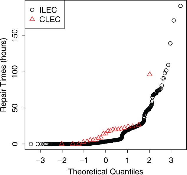
The one-sided permutation test p-value is 0.0171, well above the 1% cutoff mandated by the PUC. In comparison, the pooled t-test p-value is 0.0045, about four times too small. The permutation test gives the correct answer, with nearly exact Type 1 error rates; this was recognized as far back as Fisher (1936), who used t-tests as an approximation because perturbation tests were computationally infeasible then. The t-test is inaccurate because it is sensitive to skewness when the sample sizes differ. Using t-tests for < ![CDATA[10, 000]] > Verizon fairness tests would result in about 400 false positive results instead of the expected 100, resulting in large monetary penalties. Similarly, t confidence intervals are inaccurate. We will see how inaccurate, and explore alternatives, using the bootstrap.

1.2. One-Sample Bootstrap

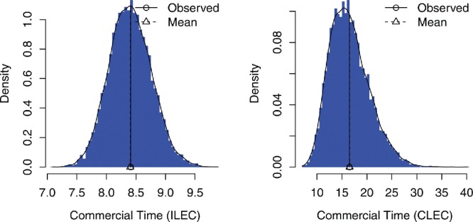
Let $\widehat{\theta }$ be a statistic calculated from a sample of n iid observations (time series and other dependent data are beyond the scope of this article). In the ordinary nonparametric bootstrap, we draw n observations with replacement from the original data to create a bootstrap sample or resample, and calculate the statistic ${\widehat{\theta }}^{*}$ for this sample (we use * to denote a bootstrap quantity). We repeat that many times, say $r=10\text{,}000$ (we use 10,000 unless noted otherwise). The bootstrap statistics comprise the bootstrap distribution. Figure 2 shows bootstrap distributions of $\widehat{\theta }=\bar{x}$ for the ILEC and CLEC datasets. We use each distribution to estimate certain things about the corresponding sampling distribution, including:

• standard error: the bootstrap standard error is the sample standard deviation of the bootstrap distribution, $s_b=\sqrt{1/(r-1){\sum }_{i=1}^r{({\widehat{\theta }}_i^{*}-\overline{{\widehat{\theta }}^{*}})}^2}$.

• confidence intervals: a quick-and-dirty interval, the bootstrap percentile interval, is the range of the middle 95% of the bootstrap distribution,

• bias: the bootstrap bias estimate is $\overline{{\widehat{\theta }}^{*}}-\widehat{\theta }$.

Figure 2 . Bootstrap distributions for Verizon data. Bootstrap distributions for $\bar{x}$, for the ILEC and CLEC datasets.

Summary statistics of the bootstrap distributions are

•  Observed SE Mean Bias

• CLEC 16.50913 3.961816 16.53088  0.0217463

• ILEC  8.41161 0.357599  8.40411 -0.0075032

The CLEC SE is larger primarily due to the smaller sample size and secondly to the larger sample sd in the original data. Bootstrap percentile intervals are (7.73, 9.13) for ILEC and (10.1, 25.4) for CLEC. For comparison, $s/\sqrt{n}=0.36$ for ILEC and 4.07 for CLEC, and standard t intervals are (7.71, 9.12) and (8.1, 24.9). The distribution appears approximately normal for the ILEC sample but not for the smaller CLEC sample, suggesting that t intervals might be reasonable for the ILEC mean but not the CLEC mean.

The bootstrap separates the concept of a standard error—the standard deviation of a sampling distribution—from the common formula $s/\sqrt{n}$ for estimating the SE of a sample mean. This separation should help students understand the concept. Based on extensive experience interviewing job candidates, I attest that a better way to teach about SEs is needed—too many do not understand SEs, and even confuse SEs in other contexts with the formula for the SE of a sample mean.

1.3. Two-Sample Bootstrap

For a two-sample bootstrap, we independently draw bootstrap samples with replacement from each sample, and compute a statistic that compares the samples. For the Verizon data, we draw a sample of size 1664 from the ILEC data and 23 from the CLEC data, and compute the difference in means ${\bar{x}}_1-{\bar{x}}_2$. The bootstrap distribution (see online supplement) is centered at the observed statistic; it is used for confidence intervals and standard errors. It is skewed like the CLEC distribution; t intervals would not be appropriate.

For comparison, the permutation test pools the data and splits the pooled data into two groups using sampling without replacement, before taking the difference in means. The sampling is consistent with the null hypothesis of no difference between groups, and the distribution is centered at zero.

1.4. Bootstrap t-Distribution

It is not surprising that t procedures are inaccurate for skewed data with a sample of size 23, or for the difference when one sample is that small. More surprising is how bad t confidence intervals are for the larger sample, size 1664. To see this, we bootstrap t statistics.

Above we resampled univariate distributions of estimators like $\bar{x}$ or ${\bar{x}}_1-{\bar{x}}_2$. Here, we look at joint distributions, for example, the joint distribution of $\bar{X}$ and s, and distributions of statistics that depend on both $\widehat{\theta }$ and θ. To estimate the sampling distribution of $\widehat{\theta }-\theta$, we use the bootstrap distribution of ${\widehat{\theta }}^{*}-\widehat{\theta }$. The bootstrap bias estimate is $E({\widehat{\theta }}^{*}-\widehat{\theta })$, an estimate of $E(\widehat{\theta }-\theta )$. To estimate the sampling distribution of a t statistic

$$\begin{array}{c}\hfill t=\frac{\widehat{\theta }-\theta }{\text{SE}},\end{array}$$ (1)

where $\text{SE}$ is a standard error calculated from the original sample, we use the bootstrap distribution of

$$\begin{array}{c}\hfill t^{*}=\frac{{\widehat{\theta }}^{*}-\widehat{\theta }}{{\text{SE}}^{*}}.\end{array}$$ (2)

Figure 3 shows the joint distribution of ${\bar{X}}^{*}$ and $s^{*}/\sqrt{n}$, and the distribution of t*, for the ILEC data with n = 1664. Standard theory says that for normal populations $\bar{X}$ and s are independent, and the t statistic $t=(\bar{X}-\mu )/(s/\sqrt{n})$ has a t-distribution. However, for positively skewed populations $\bar{X}$ and s are positively correlated, the correlation does not get smaller with large n, and the t statistic does not have a t-distribution. While ${\bar{X}}^{*}$ is positively skewed with mean $\bar{x}$, t is twice as skewed in the opposite direction because the denominator $s/\sqrt{n}$ is more affected by large observations than the numerator $\bar{X}$ is. And t has a negative median, so its quantiles end up 3x as asymmetrical to the left.

Figure 3 . CLT with n = 1664. Left: scatterplot of bootstrap means and standard errors, ILEC data. Right: bootstrap t-distribution.

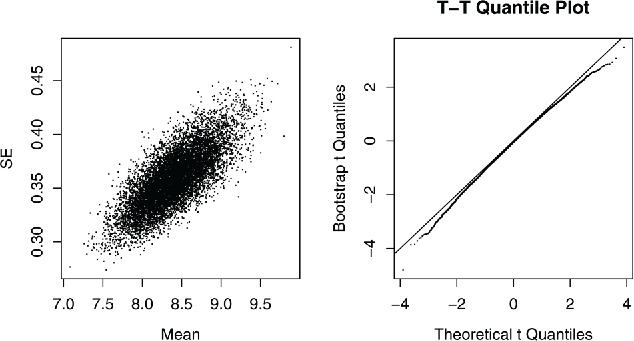
The amount of skewness apparent in the bootstrap t-distribution matters. The bootstrap distribution is a sampling distribution, not raw data; the CLT has already had its one chance to work. At this point, any deviations indicate errors in procedures that assume normal or t sampling distributions. 3.6% of the bootstrap distribution is below − t _{α/2, n − 1}, and 1.7% is above t _{α/2, n − 1} (based on r = 10⁶ samples, α = 0.05). Even with n = 1664, the t statistic is not even close to having a t-distribution, based on what matters—tail probabilities.

In my experience giving talks and courses, typically over half of the audience indicates there is no problem with the skewness apparent in plots like Figure 3. They are used to looking at normal quantile plots of data, not of sampling distributions. A common flaw in statistical practice is to fail to judge how accurate standard CLT-based methods are for specific data; the bootstrap t-distribution provides an effective way to do so.

1.5. Pedagogical and Practical Value

The bootstrap process reinforces the central role that sampling from a population plays in statistics. Sampling variability is visible, and it is natural to measure the variability of the bootstrap distribution using methods students learned for summarizing data, such as the standard deviation. Students can see if the bootstrap distribution is bell-shaped. It is natural to use the middle 95% of the distribution as a 95% confidence interval.

The bootstrap makes the abstract concrete—abstract concepts like sampling distributions, standard errors, bias, central limit theorem, and confidence intervals are visible in plots of the bootstrap distribution.

The bootstrap works the same way with a wide variety of statistics. This makes it easy for students to work with a variety of statistics, and focus on ideas rather than formulas. This also lets us do better statistics, because we can work with statistics that are appropriate rather than just those that are easy—for example, a median or trimmed mean instead of a mean.

Students can obtain confidence intervals by working directly with the statistic of interest, rather than using a t statistic. You could skip talking about t statistics and t intervals, or defer that until later. At that point you may introduce another quick-and-dirty confidence interval, the t interval with bootstrap standard error, $\widehat{\theta }\pm t_{\alpha /2}{s}_b$. In mathematical statistics, students can use the bootstrap to help understand joint distributions of estimators like $\bar{X}$ and s, and to understand the distribution of t statistics, and compute bootstrap t confidence intervals, see Section 4.3.

The bootstrap can also reinforce the understanding of formula methods, and provide a way for students to check their work. Students may know the formula $s/\sqrt{n}$ without understanding what it really is; but they can compare it to s_b or to an eyeball estimate of standard deviation from a histogram of the bootstrap distribution, and see that it measures how the sample mean varies due to random sampling.

Resampling is also important in practice. It often provides the only practical way to do inference—when it is too difficult to derive formulas, or the data are stored in a way that make calculating the formulas impractical; a longer version of this article (Hesterberg 2014) and (Chamandy 2015) contains examples from Google, from my work and others. In other cases, resampling provides better accuracy than formula methods. For one simple example, consider confidence intervals for the variance of the CLEC population. s ² = 380.4, the bootstrap SE for s ² is 267, and the 95% percentile interval is (59, 932). The classical normal-based interval is ((n − 1)s ²/χ² _{22, 0.975}, (n − 1)s ²/χ² _{22, 0.025}) = (228, 762). It assumes that (n − 1)s ²/σ² ∼ χ²(n − 1), but for long-tailed distributions the actual variance of s ² is far greater than for normal distributions. I recommend not teaching the χ² intervals for a variance, or F-based intervals for the ratio of variances, because they are not useful in practice, with no robustness against nonnormality. Their coverage does not improve as n → ∞.

2. THE IDEA BEHIND BOOTSTRAPPING

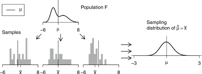
Inferential statistics is based on sampling distributions. In theory, to get these we

• draw (all or infinitely many) samples from the population, and

• compute the statistic of interest for each sample (such as the mean, median, etc.).

The distribution of the statistics is the sampling distribution, see Figure 4.

Figure 4 . Ideal world. Sampling distributions are obtained by drawing repeated samples from the population, computing the statistic of interest for each, and collecting (an infinite number of) those statistics as the sampling distribution.

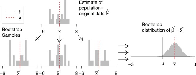
However, in practice we cannot draw arbitrarily many samples from the population; we have only one sample. The bootstrap idea is to draw samples from an estimate of the population, in lieu of the population:

• draw samples from an estimate of the population, and

• compute the statistic of interest for each sample.

The distribution of the statistics is the bootstrap distribution, see Figure 5.

Figure 5 . Bootstrap world. The bootstrap distribution is obtained by drawing repeated samples from an estimate of the population, computing the statistic of interest for each, and collecting those statistics. The distribution is centered at the observed statistic ($\bar{x}$), not the parameter (μ).

2.1. Plug-In Principle

The bootstrap is based on the plug-in principle—if something is unknown, we substitute an estimate for it. This principle is very familiar to statisticians. For example, the sd of the sample mean is $\sigma /\sqrt{n}$; when σ is unknown we substitute an estimate s, the sample standard deviation. With the bootstrap we go one step farther—instead of plugging in an estimate for a single parameter, we plug in an estimate for the whole population F.

This raises the question of what to substitute for F. Possibilities include the nonparametric, parametric, and smoothed bootstrap. The primary focus of this article is the nonparametric bootstrap, the most common procedure, which consists of drawing samples from the empirical distribution ${\widehat{F}}_n$ (with probability 1/n on each observation), that is, drawing samples with replacement from the data.

In the parametric bootstrap, we assume a model (e.g., a gamma distribution with unknown shape and scale), estimate parameters for that model, then draw bootstrap samples from the model with those estimated parameters.

The smoothed bootstrap is a compromise between parametric and nonparametric approaches; if we believe the population is continuous, we may sample from a continuous $\widehat{F}$, say a kernel density estimate (Silverman and Young 1987; Hall, DiCiccio, and Romano 1989; Hesterberg 2014). Smoothing is not common; it is rarely needed, and does not generalize well to multivariate and factor data.

2.2. Fundamental Bootstrap Principle

The fundamental bootstrap principle is that this substitution usually works—that we can plug in an estimate for F, then sample, and the resulting bootstrap distribution provides useful information about the sampling distribution.

The bootstrap distribution is in fact a sampling distribution. The bootstrap uses a sampling distribution (from an estimate $\widehat{F}$) to estimate things about the sampling distribution (from F).

There are some things to watch out for, ways the bootstrap distribution differs from the sampling distribution. We discuss some of these below, but one is important enough to mention immediately.

2.3. Inference, Not Better Estimates

The bootstrap distribution is centered at the observed statistic, not the population parameter, for example, at $\bar{x}$, not μ.

This has two profound implications. First, it means that we do not use the mean of the bootstrap statistics as a replacement for the original estimate. ¹ For example, we cannot use the bootstrap to improve on $\bar{x}$; no matter how many bootstrap samples we take, they are centered at $\bar{x}$, not μ. Instead we use the bootstrap to tell how accurate the original estimate is. In this regard the bootstrap is like formula methods that use the data twice—once to compute an estimate, and again to compute a standard error for the estimate. The bootstrap just uses a different approach to estimating the standard error.

If the bootstrap distribution is not centered at the observed statistic—if there is bias—we could subtract the estimated bias to produce a bias-adjusted estimate, $\widehat{\theta }-\widehat{\text{Bias}}=2\widehat{\theta }-\overline{{\widehat{\theta }}^{*}}$. We generally do not do this—bias estimates can have high variability (Efron and Tibshirani 1993). Bias is another reason not to use the average of bootstrap estimates $\overline{{\widehat{\theta }}^{*}}=\widehat{\theta }+\widehat{\text{Bias}}$ to replace the original estimate $\widehat{\theta }$—that adds the bias estimate to the original statistic, doubling any bias.

The second implication is that we do not use the CDF or quantiles of the bootstrap distribution of ${\widehat{\theta }}^{*}$ to estimate the CDF or quantiles of the sampling distribution of an estimator $\widehat{\theta }$. Instead, we bootstrap to estimate things like the standard deviation, the expected value of $\widehat{\theta }-\theta$, and the CDF and quantiles of $\widehat{\theta }-\theta$ or $(\widehat{\theta }-\theta )/\text{SE}$.

2.4. Key Idea Versus Implementation Details

What people may think of as the key bootstrap idea—drawing samples with replacement from the data—is just a pair of implementation details. The first is substituting the empirical distribution for the population; alternatives include smoothed or parametric distributions. The second is using random sampling. Here too there are alternatives, including analytical methods (e.g., when $\widehat{\theta }=\bar{x}$ we may calculate the mean and variance of the bootstrap distribution analytically) and exhaustive calculations. There are nⁿ possible bootstrap samples from a fixed sample of size n, $\left(\genfrac{}{}{0pt}{}{2n-1}{n}\right)$ if order does not matter, or even fewer in some cases like binary data; if n is small we could evaluate all of these. We call this an exhaustive bootstrap or theoretical bootstrap. But more often exhaustive methods are infeasible, so we draw say 10,000 random samples instead; we call this the Monte Carlo sampling implementation.

2.5. How to Sample

Normally we should draw bootstrap samples the same way the sample was drawn in real life, for example, simple random sampling or stratified sampling. Pedagogically, this reinforces the role that random sampling plays in statistics.

One exception to that rule is to condition on the observed information. For example, when comparing samples of size n ₁ and n ₂, we fix those numbers, even if the original sampling process could have produced different counts. (This is the conditionality principle in statistics, the idea of conditioning on ancillary statistics.) Conditioning also avoids some technical problems, particularly in regression, see Section 5.

We can also modify the sampling to answer what-if questions. For example, we could bootstrap with and without stratification and compare the resulting standard errors, to investigate the value of stratification. We could also draw samples of a different size; say we are planning a large study and obtain an initial dataset of size 100, we can draw bootstrap samples of size 2000 to estimate how large standard errors would be with that sample size. Conversely, this also answers a common question about bootstrapping—why we sample with the same size as the original data—because by doing so the standard errors reflect the actual data, rather than a hypothetical larger or smaller dataset.

3. VARIATION IN BOOTSTRAP DISTRIBUTIONS

We claimed above that the bootstrap distribution usually provides useful information about the sampling distribution. We elaborate on that now with a series of visual examples, one where things generally work well and three with problems. We address two questions:

• How accurate is the theoretical (exhaustive) bootstrap?

• How accurately does the Monte Carlo implementation approximate the theoretical bootstrap?

Both reflect random variation:

• The original sample is chosen randomly from the population.

• Bootstrap resamples are chosen randomly from the original sample.

3.1. Sample Mean: Large Sample Size

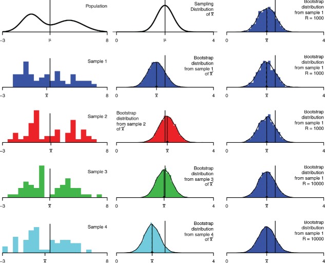
Figure 6 shows a population, the sampling distribution for the mean with n = 50, four samples, and the corresponding bootstrap distributions. Each bootstrap distribution is centered at the statistic $\bar{x}$ from the corresponding sample rather than at the population mean μ. The spreads and shapes of the bootstrap distributions vary a bit but not a lot.

Figure 6 . Bootstrap distribution for the mean, n = 50. The left column shows the population and four samples. The middle column shows the sampling distribution for $\bar{X}$, and bootstrap distributions of ${\bar{X}}^{*}$ for each sample, with r = 10⁴. The right column shows more bootstrap distributions for the first sample, three with r = 1000 and two with r = 10⁴.

These observations inform what the bootstrap distributions may be used for. The bootstrap does not provide a better estimate of the population parameter, because the bootstrap means are centered at $\bar{x}$, not μ. Similarly, quantiles of the bootstrap distributions are not useful for estimating quantiles of the sampling distribution. Instead, the bootstrap distributions are useful for estimating the spread and shape of the sampling distribution.

The right column shows additional bootstrap distributions for the first sample, with r = 1000 or r = 10⁴ resamples. Using more resamples reduces random Monte Carlo variation, but does not fundamentally change the bootstrap distribution—it still has the same approximate center, spread, and shape.

The Monte Carlo variation is much smaller than the variation due to different original samples. For many uses, such as quick-and-dirty estimation of standard errors or approximate confidence intervals, r = 1000 resamples is adequate. However, there is noticeable variability (including important but less-noticeable variability in the tails) so when accuracy matters, r = 10⁴ or more samples should be used.

3.2. Sample Mean: Small Sample Size

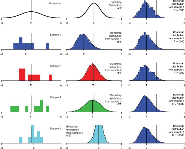
Figure 7 is similar to Figure 6, but for a smaller sample size, n = 9 (and a different population). As before, the bootstrap distributions are centered at the corresponding sample means, but now the spreads and shapes of the bootstrap distributions vary substantially, because the spreads and shapes of the samples vary substantially. As a result, bootstrap confidence interval widths vary substantially (this is also true of standard t confidence intervals). As before, the Monte Carlo variation is small and may be reduced with more resamples.

Figure 7 . Bootstrap distributions for the mean, n = 9. The left column shows the population and four samples. The middle column shows the sampling distribution for $\bar{X}$, and bootstrap distributions of ${\bar{X}}^{*}$ for each sample, with r = 10⁴. The right column shows more bootstrap distributions for the first sample, three with r = 1000 and two with r = 10⁴.

While not apparent in the pictures, bootstrap distributions tend to be too narrow on average, by a factor of $\sqrt{(n-1)/n}$ for the sample mean, and approximately that for many other statistics. This goes back to the plug-in principle; the empirical distribution has variance ${\widehat{\sigma }}^2={\text{var}}_{{\widehat{F}}_n}\left(X\right)=1/n\sum {(x_i-\bar{x})}^2$, and the theoretical bootstrap standard error is the standard deviation of a mean of n independent observations from that distribution, $s_b=\widehat{\sigma }/\sqrt{n}$. That is, smaller than the usual formula $s/\sqrt{n}$ by a factor of $\sqrt{(n-1)/n}$. For example, the CLEC s_b = 3.96 is smaller than $s/\sqrt{n}=4.07$.

The combination of this narrowness bias and variability in spread makes some bootstrap confidence intervals under-cover, see Section 4. Classical t intervals compensate using two fudge factors—a factor of $\sqrt{n/(n-1)}$ in computing the sample standard deviation s, and using t rather than normal quantiles. Bootstrap percentile intervals lack these factors, so tend to be too narrow and under-cover in small samples. t intervals with bootstrap SE include the t/z factor, but suffer narrowness bias. Some other bootstrap procedures do better. For Stat 101 I suggest warning students about the issue; for higher courses you may discuss remedies (Hesterberg 2004, 2014).

In two-sample or stratified sampling situations, the narrowness bias depends on the individual sample or strata sizes. This can result in severe bias. For example, the U.K. Department of Work and Pensions wanted to bootstrap a survey of welfare cheating. They used a stratified sampling procedure that resulted in two subjects in each stratum—so an uncorrected bootstrap standard error would be too small by a factor of $\sqrt{(n_i-1)/n_i}=\sqrt{1/2}$.

3.3. Sample Median

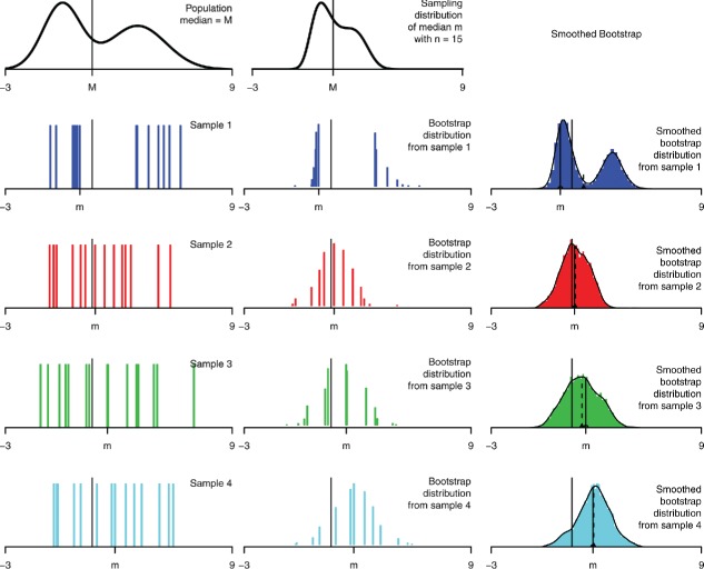
Now turn to Figure 8, where the statistic is the sample median. Here the bootstrap distributions are poor approximations of the sampling distribution. The sampling distribution is continuous, but the bootstrap distributions are discrete—for odd n the bootstrap sample median is always one of the original observations—and with wildly varying shapes.

Figure 8 . Bootstrap distributions for the median, n = 15. The left column shows the population and four samples. The middle column shows the sampling distribution, and bootstrap distributions for each sample, with r = 10⁴. The right column shows smoothed bootstrap distributions, with kernel sd $s/\sqrt{n}$ and r = 10⁴.

The ordinary bootstrap tends not to work well for statistics such as the median or other quantiles in small samples that depend heavily on a small number of observations out of a larger sample. The bootstrap depends on the sample accurately reflecting what matters about the population, and those few observations cannot do that. The right column shows the smoothed bootstrap; it is better, though is still poor for this small n.

In spite of the inaccurate shape and spread of the bootstrap distributions, the bootstrap percentile interval for the median is not bad (Efron 1982). For odd n, percentile interval endpoints fall on one of the observed values. Exact interval endpoints also fall on one of the observed values (order statistics), and for a 95% interval those are typically the same or adjacent order statistics as the percentile interval.

3.4. Mean–Variance Relationship

In many applications, the spread or shape of the sampling distribution depends on the parameter of interest. For example, the binomial distribution spread and shape depend on p. Similarly, for an exponential distribution, the standard deviation of the sampling distribution of $\bar{x}$ is proportional to μ.

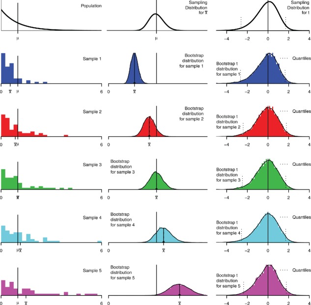
This mean–variance relationship is reflected in bootstrap distributions. Figure 9 shows samples and bootstrap distributions for an exponential population. There is a strong dependence between $\bar{x}$ and the corresponding bootstrap SE. This relationship has important implications for confidence intervals; procedures that ignore the relationship are inaccurate. We discuss this more in Section 4.5.

Figure 9 . Bootstrap distributions for the mean, n = 50, exponential population. The left column shows the population and five samples. (These samples are selected from a larger set of random samples, to have means spread across the range of sample means, and average standard deviations conditional on the means.) The middle column shows the sampling distribution and bootstrap distributions for each sample. The right column shows bootstrap t-distributions.

There are other applications where sampling distributions depend strongly on the parameter, for example, sampling distributions for chi-squared statistics depend on the noncentrality parameter. Use caution when bootstrapping such applications; the bootstrap distribution may be very different from the sampling distribution.

Here there is a bright spot. The right column of Figure 9 shows the sampling distribution and bootstrap distributions of the t statistic, Equations (1) and (2). These distributions are much less sensitive to the original sample. We use these bootstrap t distributions below to construct accurate confidence intervals.

3.5. Summary of Visual Lessons

The bootstrap distribution reflects the original sample. If the sample is narrower than the population, the bootstrap distribution is narrower than the sampling distribution. Typically for large samples the data represent the population well; for small samples they may not. Bootstrapping does not overcome the weakness of small samples as a basis for inference. Indeed, for the very smallest samples, it may be better to make additional assumptions such as a parametric family.

Looking ahead, two things matter for accurate inferences:

• how close the bootstrap distribution is to the sampling distribution (the bootstrap t has an advantage, see Figure 9);

• how well the procedures allow for variation in samples, for example, by using fudge factors.

Another visual lesson is that random sampling using only 1000 resamples causes more random variation in the bootstrap distributions. Let us consider this issue more carefully.

3.6. How Many Bootstrap Samples

I suggested above using 1000 bootstrap samples for rough approximations, or 10⁴ or more for better accuracy. This is about Monte Carlo accuracy—how well the usual Monte Carlo implementation of the bootstrap approximates the theoretical bootstrap distribution. A bootstrap distribution based on r random samples corresponds to drawing r observations with replacement from the theoretical bootstrap distribution.

Brad Efron, inventor of the bootstrap, suggested in 1993 that r = 200, or even as few as r = 25, suffices for estimating standard errors and that r = 1000 is enough for confidence intervals (Efron and Tibshirani 1993).

I argue that more resamples are appropriate. First, computers are faster now. Second, those criteria were developed using arguments that combine variation due to the original random sample with the extra variation from the Monte Carlo implementation. I prefer to treat the data as given and look just at the variability due to the implementation. Two people analyzing the same data should not get substantially different answers due to Monte Carlo variation.

Quantify accuracy by formulas or bootstrapping

We can quantify the Monte Carlo variation in two ways—using formulas, or by bootstrapping. For example, let G be the cdf of a theoretical bootstrap distribution and $\widehat{G}$ the Monte Carlo approximation, then the variance of $\widehat{G}\left(x\right)$ is G(x)(1 − G(x))/r, which we estimate using $\widehat{G}\left(x\right)(1-\widehat{G}\left(x\right))/r$.

Similarly, a bootstrap bias estimate is a mean of r random values minus a constant, $\overline{{\widehat{\theta }}^{*}}-\widehat{\theta }$; the Monte Carlo standard error for the bias is $s_b/\sqrt{r}$, where s_b is the sample standard deviation of the bootstrap distribution.

We can also bootstrap the bootstrap distribution! The r bootstrap statistics are an iid sample from the exhaustive bootstrap distribution; we can bootstrap that sample. For example, the 95% percentile confidence interval for the CLEC data is (10.09, 25.41); these are 2.5% and 97.5% quantiles of the bootstrap distribution; r = 10⁴. To estimate the accuracy of those quantiles, we draw resamples of size r from the bootstrap distribution and compute the quantiles for each resample. The resulting SEs for the quantile estimates are 0.066 and 0.141.

Need r ≥ 15,000 to be within 10%.  Next we determine how large r should be for accurate results, beginning with two-sided tests with size 5%. Suppose the true one-sided p-value is 0.025, and we want the estimated p-value to be within 10% of that, between 0.0225 and 0.0275. To have a 95% probability of being that close requires that $1.96\sqrt{0.025·0.975/r}<0.025/10$, or r ⩾ 14, 982. Similar results hold for a bootstrap percentile or bootstrap t confidence interval. If q is the true 2.5% quantile of the theoretical bootstrap distribution (for ${\widehat{\theta }}^{*}$ or t*, respectively), for the estimated $\widehat{G}\left(q\right)$ to fall between 2.25% and 2.75% with 95% probability requires $r\ge 14\text{,}982$.

For a t interval with bootstrap SE, r should be large enough that variation in s_b has a similar small effect on coverage. For large n and an approximately normal bootstrap distribution, about r ⩾ 5000 suffices (Hesterberg 2014).

Rounding up, we need $r\ge 15\text{,}000$ to have 95% probability of being within 10%, for permutation tests and percentile and bootstrap t confidence intervals, and r ⩾ 5000 for the t with bootstrap SE. While students may not need this level of accuracy, it is good to get in the habit of doing accurate simulations. Hence, I recommend 10⁴ for routine use. In practice, if the results with r = 10⁴ are borderline, then we can increase r to reduce the Monte Carlo error. We want decisions to depend on the data, not random variation in the Monte Carlo implementation. We used $r=500\text{,}000$ in the Verizon project.

Students can do multiple runs with different r, to see how the results vary. They should develop some intuition into how results vary with different r; this intuition is valuable not only for resampling, but for general understanding of how estimates vary for different n.

4. CONFIDENCE INTERVALS

In this section, I describe a number of confidence intervals, and compare their pedagogical value and accuracy.

A hypothesis test or confidence interval is first-order accurate if the actual one-sided rejection probabilities or one-sided noncoverage probabilities differ from the nominal values by O(n ^{− 1/2}). It is second-order accurate if the differences are O(n ^{− 1}).

4.1. Statistics 101—Percentile, and t with Bootstrap SE

For Stat 101, I would stick with the two quick-and-dirty intervals mentioned earlier: the bootstrap percentile interval, and the t interval with bootstrap standard error $\widehat{\theta }\pm t_{\alpha /2}{s}_b$. If using software that provides it, you may also use the bootstrap t interval described below. The percentile interval will be more intuitive for students. The t with bootstrap standard error helps them learn formula methods. Students can compute both and compare.

Neither interval is very accurate. They are only first-order accurate, and are poor in small samples—they tend to be too narrow. The bootstrap standard error is too small, by a factor $\sqrt{(n-1)/n}$ so the t interval with bootstrap SE is too narrow by that factor, this is, the narrowness bias discussed in Section 3.2.

The percentile interval suffers the same narrowness and more—for symmetric data it is like using $z_{\alpha /2}\widehat{\sigma }/\sqrt{n}$ in place of $t_{\alpha /2,n-1}s/\sqrt{n}$. Random variability in how skewed the data are also adds variability to the endpoints, further reducing coverage. These effects are O(n ^{− 1}) (effect on coverage probability) or smaller, so they become negligible fairly quickly as n increases. But they matter for small n, see Figure 10. The interval also has O(n ^{− 1/2}) errors—because it only makes a partial skewness correction, see Section 4.5.

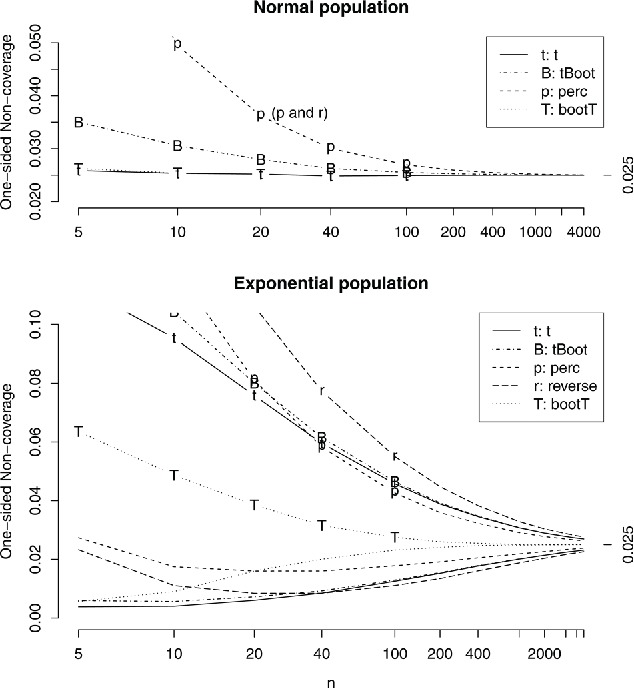
Figure 10 . Confidence interval one-sided miss probabilities for normal and exponential populations. 95% confidence interval, the ideal noncoverage is 2.5% on each side. The intervals are described at the beginning of Section 4.4. For the normal population noncoverage probabilities are the same on both sides, and the reverse percentile interval is omitted (it has the same coverage as the percentile interval). For the exponential population, curves with letters are noncoverage probabilities on the right, where the interval is below θ, and curves without letters correspond to the left side.

In practice, the t with bootstrap standard error offers no advantage over a standard t procedure for the sample mean. Its advantages are pedagogical, and that it can be used for statistics that lack easy standard error formulas.

The percentile interval is not a good alternative to standard t intervals for the mean of small samples—while it handles skewed populations better, it is less accurate for small samples because it is too narrow. For exponential populations, the percentile interval is less accurate than the standard t interval for n ⩽ 34.

In Stat 101, it may be best to avoid the small-sample problems by using examples with larger n. Alternately, some software corrects for the small-sample problems, for example, the resample package (Hesterberg 2015) includes the expanded percentile interval (Hesterberg 1999, 2014) a percentile interval with fudge factors motivated by standard t intervals.

4.2. Reverse Bootstrap Percentile Interval

The reverse bootstrap percentile interval (called “basic bootstrap confidence interval” in Davison and Hinkley 1997) is a common interval, with pedagogical value in teaching manipulations like those shown just below. But it is poor in practice; I include it here to help faculty and students understand why and to discourage its use.

It is based on the distribution of $\widehat{\delta }=\widehat{\theta }-\theta$. We estimate the CDF of $\widehat{\delta }$ using the bootstrap distribution of ${\widehat{\delta }}^{*}={\widehat{\theta }}^{*}-\widehat{\theta }$. Let q _α be the α quantile of the bootstrap distribution of ${\widehat{\delta }}^{*}$, that is, $\alpha =P({\widehat{\delta }}^{*}\le q_{\alpha })$. Then

$$\begin{array}{ccc}\hfill \alpha /2& =& P({\widehat{\theta }}^{*}-\widehat{\theta }<q_{\alpha /2})\hfill \\ & \approx & P(\widehat{\theta }-\theta <q_{\alpha /2})=P(\widehat{\theta }-q_{\alpha /2}<\theta ).\hfill \end{array}$$

Similarly for the other tail. The resulting confidence interval is

$$\begin{array}{c}\hfill (\widehat{\theta }-q_{1-\alpha /2},\widehat{\theta }-q_{\alpha /2})=(2\widehat{\theta }-Q_{1-\alpha /2},2\widehat{\theta }-Q_{\alpha /2}),\end{array}$$ (3)

where Q _α is the quantile of the bootstrap distribution of ${\widehat{\theta }}^{*}$.

This interval is the mirror image of the bootstrap percentile interval; it reaches as far above $\widehat{\theta }$ as the bootstrap percentile interval reaches below. For example, for the CLEC mean, the sample mean is 16.5, the percentile interval is (10.1, 25.4) = 16.5 + ( − 6.4, 8.9), and the reverse percentile interval is 16.5 + ( − 8.9, 6.4) = 2 · 16.5 − (25.4, 10.1) = (7.6, 22.9).

Reversing works well for a pure translation family, but those are rare in practice. More common are cases like Figure 9, where the spread of the bootstrap distribution depends on the statistic. Then a good interval needs to be asymmetric in the same direction as the data, see Section 4.5. The reverse percentile interval is asymmetrical in the wrong direction! Its coverage accuracy in Figure 10 is terrible. It also suffers from the same small-sample narrowness issues as the percentile interval.

Hall (1992) called the bootstrap percentile interval “the wrong pivot, backward”; the reverse percentile interval uses that same wrong pivot in reverse. $\widehat{\delta }$ is the wrong pivot because it is not even close to pivotal—a pivotal statistic is one whose distribution is independent of the parameter. A t statistic is closer to pivotal; this leads us to the next interval.

4.3. Bootstrap t Interval

We saw in Section 1.4 that the t statistic does not have a t-distribution when the population is skewed. The bootstrap t confidence interval is based on the t statistic, but estimates quantiles of the actual distribution using the data rather than a table. Efron and Tibshirani (1993) called this “Confidence intervals based on bootstrap tables”—using the bootstrap to generate the right table for an individual dataset, rather than using a table from a book. This has the best coverage accuracy of all intervals in Figure 10.

We assume that the distribution of t* is approximately the same as the distribution of t (Equations (1) and (2)); the right column of Figure 9 suggests that this assumption holds, that is, the statistic is close to pivotal. Let q _α be the α quantile of the bootstrap t-distribution, then

$$\begin{array}{ccc}\hfill \alpha /2& =& P\left(\frac{{\widehat{\theta }}^{*}-\widehat{\theta }}{{\text{SE}}^{*}}<q_{\alpha /2}\right)\hfill \\ & \approx & P\left(\frac{\widehat{\theta }-\theta }{\text{SE}}<q_{\alpha /2}\right)=P(\widehat{\theta }-q_{\alpha /2}\text{SE}<\theta ).\hfill \end{array}$$

Similarly for the other tail. The resulting confidence interval is

$$\begin{array}{c}\hfill (\widehat{\theta }-q_{1-\alpha /2}\text{SE},\widehat{\theta }-q_{\alpha /2}\text{SE}).\end{array}$$ (4)

Note that endpoints are reversed: we subtract an upper quantile of the bootstrap t-distribution to get the lower endpoint of the interval, and the converse (this reversal is easy to overlook with standard t intervals due to symmetry).

4.4. Confidence Interval Accuracy

Next we compare the accuracy of the different confidence intervals:

• t = t: ordinary t interval;

• B = tBoot: t interval with bootstrap standard error;

• p = perc: bootstrap percentile interval;

• r = reverse: reverse percentile interval;

• T = bootT: bootstrap t.

For a 95% interval, a perfectly accurate interval misses the parameter 2.5% of the time on each side. Figure 10 shows actual noncoverage probabilities for normal and exponential populations, respectively. The figure is based on extremely accurate simulations, see the appendix.

Normal population.  The percentile interval (“p” on the plot) does poorly. It corresponds to using z instead of t, using a divisor of n instead of n − 1 when calculating SE, and doing a partial correction for skewness; since the sample skewness is random this adds variability. For normal data the skewness correction does not help, and the other three things kill it for small samples. The reverse percentile interval is similarly poor, with exactly the same coverage for normal populations.

The t interval with bootstrap SE (“B”) does somewhat better, though still under-covers. The t interval (“t”) and bootstrap t (“T”) interval do very well. That is not surprising for the t interval, which is optimized for this population, but the bootstrap t does extremely well, even for very small samples.

Exponential population.  This is a harder problem. All intervals badly under-cover on the right—the intervals are too short on the right side—and over-cover (by smaller amounts) on the left. (Over-covering on one side does not compensate for under-covering on the other—instead, having both endpoints too low gives an even more biased picture about where the parameter may be than having just one endpoint too low.)

The bootstrap t interval (“T”) does best, by a substantial margin. It is second-order accurate, and gives coverage within 10% for n ⩾ 101. The other intervals are all poor. The reverse percentile interval (“r”) is the worst. The percentile interval (“p”) is poor for small samples, but better than the ordinary t (“t”) for n ⩾ 35. To reach 10% accuracy requires n ⩾ 2383 for percentile, 4815 for ordinary t, 5063 for t with bootstrap standard errors, and over 8000 for the reverse percentile method.

4.5. Skewness and Mean–Variance Relationship

Take another look at Figure 9, for the sample mean from a skewed population. Note how the spread of the bootstrap distribution for ${\bar{x}}^{*}$ depends on the statistic $\bar{x}$. To obtain accurate confidence intervals, we need to allow for such a relationship (and Mathematical Statistics students should be aware of this).

For positively skewed populations, when $\bar{x}<\mu$ the sample standard deviation and bootstrap SE also tend to be small, so a confidence interval needs to reach many (small) SE’s to the right to avoid missing μ too often. Conversely, when $\bar{x}>\mu$, s and s_b tend to be large, so a confidence interval does not need to reach many (large) SE’s to the left to reach μ.

In fact, a good interval, like the bootstrap t interval, is even more asymmetrical than a bootstrap percentile interval—about three times as asymmetrical in the case of a 95% intervals for a mean (Hesterberg 2014). The bootstrap t explicitly estimates how many standard errors to go in each direction. This table shows how far the endpoints for the t, percentile, reverse percentile, and bootstrap t intervals are above and below the sample mean of the Verizon ILEC data:

Table NaN .

	t	Reverse	Percentile	bootstrapT
2.5%	−0.701	−0.718	−0.683	−0.646
97.5%	0.701	0.683	0.718	0.762
-ratio	1	0.951	1.050	1.180

The bootstrap percentile interval is asymmetrical in the right direction, but falls short; the reverse percentile interval goes the wrong way.

For right-skewed data, you may be surprised that good confidence intervals are 3x as asymmetrical as the bootstrap percentile interval; You may even be inclined to “downweight the outliers,” and use an interval that reaches farther left; the reverse percentile interval does so, with catastrophic effect. Instead, think of it this way: the data show that the population is skewed, take that as given; we may have observed too few observations from the long right tail, so the confidence interval needs to reach far to the right to protect against that—many (small) SE’s to the right.

4.6. Confidence Interval Details

There are different ways to compute quantiles common in statistical practice. For intervals based on quantiles of the bootstrap distribution, I recommend letting the kth largest value in the bootstrap distribution be the (k + 1)/r quantile, and interpolating for other quantiles. In R (R Core Team 2014) this is quantile(x, type=6). Other definitions give narrower intervals, and exacerbate the problem of intervals being too short.

Bootstrap t intervals require standard errors—for the original sample, and each bootstrap sample. When formula SE’s are not available, we can use the bootstrap to obtain these SE’s (Efron and Tibshirani 1993), using an iterated bootstrap, in which a set of second-level bootstrap samples is drawn from each top-level bootstrap sample to estimate the SE for that bootstrap sample. This requires r + rr ₂ resamples if r ₂ second level samples are drawn from each top-level sample. The computational cost has been an impediment, but should be less so in the future as computers make use of multiple processors.

While the simulation results here are for the sample mean, the bootstrap t is second-order accurate and the others are first-order accurate under quite general conditions, see Efron and Tibshirani (1993) and Davison and Hinkley (1997). Efron and Tibshirani (1993) noted that the bootstrap t is particularly suited to location statistics like the sample mean, median, trimmed mean, or percentiles, but performs poorly for a correlation coefficient; they obtain a modified version by using a bootstrap t for a transformed version of the statistic ψ = h(θ), where h is a variance-stabilizing transformation (so that $\text{var}\left(\widehat{\psi }\right)$ does not depend on ψ) estimated using a creative use of the bootstrap. The same method improves the reverse percentile interval (Davison and Hinkley 1997).

4.7. Bootstrap Hypothesis Testing

There are two broad approaches to bootstrap hypothesis testing. One approach is to invert a confidence interval—reject H ₀ if the corresponding interval excludes θ₀.

Another approach is to sample in a way that is consistent with H ₀, then calculate a p-value as a tail probability. For example, we could perform a two-sample bootstrap test by pooling the data and drawing bootstrap samples of size n ₁ and n ₂ with replacement from the pooled data. However, this bootstrap test is not as accurate as the permutation test. Suppose, for example, that the data contain three outliers. The permutation test tells how common the observed statistic is, given the three outliers. With a pooled bootstrap the number of outliers would vary. The permutation test conditions on the data, treating only group assignment as random.

Another example, for a one-sample mean, is to translate the data, subtracting $\bar{x}-{\mu }_0$ from each x_i so the translated mean is μ₀, then resample from the translated data. This is equivalent to inverting a reverse percentile confidence interval, with corresponding inaccuracy for skewed data. It can also yield impossible data, like negative values for data that must be positive.

Translation modifies a distribution by modifying the values. A better way to modify a distribution is to keep the same values, but change the probabilities on those values, using bootstrap tilting (Efron 1981; Davison and Hinkley 1997); empirical likelihood (Owen 2001) is related. Tilting preserves mean–variance relationships. I believe tilting has great pedagogical potential for mathematical statistics; it nicely connects parametric and nonparametric statistics, can help students understand the relationship between parameters and sampling distributions, and better understand confidence intervals. See the online supplement for an example. But suitable software for educational use is not currently available.

Neither approach is as accurate as permutation tests, in situations where permutation tests can be used. The actual one-sided rejection probabilities when inverting confidence intervals correspond to Figure 10. In contrast, permutation tests are nearly exact.

5. REGRESSION

There are two ways that bootstrapping in regression is particularly useful pedagogically. The first is to help students understand the variability of regression predictions by a graphical bootstrap. For example, in Figure 11 we bootstrap regression lines; those lines help students understand the variability of slope and intercept coefficients, and of predictions at each value of x. The more we extrapolate in either direction, the more variable the predictions become. A bootstrap percentile confidence interval for E(Y|x) is the range of the middle 95% of the y values for regression lines at any x; these intervals are wider for more extreme x.

Figure 11 . Bootstrapping linear regression. Left: Linear regression linear model fits. At any x, the y values from the bootstrap lines form a bootstrap distribution that may be used for standard errors or confidence intervals. Prediction intervals are wider, to capture individual observations. Right: Fitting a linear relationship to data that are not linear; the bootstrap does not diagnose the poor fit.

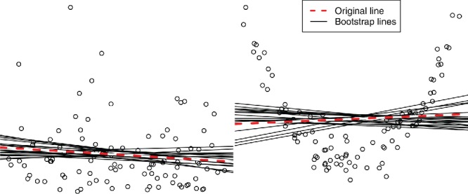
The second is to help students understand the difference between confidence and prediction intervals. In the left panel, we see that the variability of individual observations is much larger than the variability of the regression lines; confidence intervals based on the lines would capture only a small fraction of observations. To capture observations, prediction intervals must be much wider, and should approximate the quantiles of the residual distribution, because they are primarily intervals for individual observations—no CLT applies for prediction intervals.

The bootstrap estimates the performance of the model that was actually fit to the data, regardless of whether that is a poor model. In the right panel of Figure 11, a linear approximation was used even though the relationship is quadratic; the bootstrap measures the variability of the linear approximation, and estimates the bias of (a linear approximation to the data) as an estimate of (a linear approximation to the population). The bootstrap finds no bias—for any x, the bootstrap lines are centered vertically around the original fit.

5.1. Resample Observations or Conditional Distributions

Two common procedures when bootstrapping regression are

• bootstrap observations, and

• bootstrap residuals.

The latter is a special case of a more general rule:

• resample y from its estimated conditional distribution given x.

In bootstrapping observations, we sample with replacement from the observations, keeping y and corresponding x’s together. In any bootstrap sample some observations may be repeated multiple times, and others not included.

In bootstrapping residuals, we fit a regression model, compute predicted values ${\widehat{y}}_i$ and residuals $e_i=y_i-{\widehat{y}}_i$, then create a bootstrap sample using the same x values as in the original data, but with y obtained by adding the predictions and random residuals, $y_i^{*}={\widehat{y}}_i+e_i^{*}$, where e*_i are sampled randomly with replacement from the original residuals.

Bootstrapping residuals correspond to a designed experiment where the x’s are fixed and only y is random, and bootstrapping observations to randomly sampled data where both x and y are sampled from a joint distribution. By the principle of sampling the way the data were drawn, we would bootstrap observations if the x’s were random. Alternately, we can follow the precedent set by the common formula approach, where formulas are derived assuming the x’s are fixed, and in practice we use these even when the x’s are random. In doing so we condition on the observed x’s, and hence on the observed information (in regression the information depends on the spread of the x’s—the wider the spread, the less $\widehat{\beta }$ varies). Similarly, in bootstrapping, we may resample the residuals, conditioning on the observed x’s.

Fixing the x’s can make a big difference in practice; bootstrapping observations can be dangerous. For example, suppose one of the x’s is a factor variable with a rare level, say only five observations. When resampling observations, about 67 out of 10,000 samples omit those five observations entirely; then the regression software cannot estimate a coefficient for that level. Worse, many samples will include just one or two observations from that level; then the software produces estimates with high variance, with no error message to flag the problem. Similar problems occur in models with interactions, or with continuous variables when some linear combination ∑c_jx_j has most of its variation in a small number of observations. We avoid these problems by bootstrapping residuals.

Bootstrapping residuals is a special case of a more general rule, to sample Y from its estimated conditional distribution given X. For example, when bootstrapping logistic regression, we fit the model, and calculate predicted values ${\widehat{y}}_i=\widehat{E}\left(Y\right|X=x_i)=\widehat{P}(Y=1|X=x_i)$. To generate a bootstrap sample, we keep the same x’s, and let y*_i = 1 with probability ${\widehat{y}}_i$, otherwise y*_i = 0. This is an example of a parametric bootstrap. We use this at Google in a complicated multi-stage logistic regression procedure.

The conditional distribution idea also helps in linear regression where there is heteroscedasticity or lack of fit; we sample residuals from observations with similar residual distributions, for example, from observations with similar predictions (for heteroscedasticity) or x’s (for lack of fit).

6. DISCUSSION

We first summarize some points from above, then discuss books and software.

Bootstrapping offers a number of pedagogical benefits. The process of bootstrapping mimics the central role that sampling plays in statistics. Students can use familiar tools like histograms to visualize sampling distributions and standard errors. They may understand that an SE is the standard deviation of a sampling distribution. Students can work directly with estimates of interest, like sample means, instead of t statistics, and use the same basic procedure for many different statistics without new formulas. Robust statistics like medians and trimmed means can be used throughout the course. Students can focus on the ideas, not formulas. When learning formulas, they can compare formula and bootstrap answers. Graphical bootstrapping for regression demonstrates the variation in regression predictions, and the difference between confidence and prediction intervals.

Understanding the key idea behind the bootstrap—sampling from an estimate of the population—is important to use the bootstrap appropriately, and helps to understand when it may not work well, or which methods may work better. When using Monte Carlo sampling, enough samples should be used to obtain accurate answers—10,000 is good for routine use. Students can gain insight into sampling variation by trying different numbers.

Bootstrap distributions and percentile confidence intervals tend to be too narrow, particularly for small samples. As a result, percentile intervals are less accurate than common t intervals for small samples, though more accurate for larger samples. Most accurate are bootstrap t intervals. The reason relates to the fundamental idea of the bootstrap—to replace the population by an estimate of the population, then use the resulting bootstrap distribution as an estimate of the sampling distribution. This substitution is more accurate for a pivotal statistic—and the t statistic is close to pivotal.

For skewed data, confidence intervals should reach longer in the direction of the skewness; the bootstrap t does this well, the percentile makes about 1/3 of that correction, t intervals ignore skewness, and reverse percentile intervals go the wrong way.

We generally sample the way the data were produced (e.g., simple random or stratified sampling), except to condition on observed information. For regression, that means to fix the x values, that is, to resample residuals rather than observations. This avoids problems in practice.

To reach the full potential of bootstrapping in practice and education, we need better software and instructional materials. Software such as https://www.stat.auckland.ac.nz/wild/VIT or http://lock5stat.com/statkey has a place in education, to help students visualize the sampling process, but is not suitable when students go into real jobs. In R (R Core Team 2014), students can write bootstrap loops from scratch, but this is difficult for Stat 101 students. For that matter it may be difficult for higher level students, but it is worth putting in that effort. Modern statistics requires extensive computing skills including resampling and simulation (ASA 2014), and developing those skills should start early. The Mosaic package (Pruim, Kaplan, and Horton 2015) can make this easier, and the package contains one vignette for resampling and another with resources including supplements using Mosaic for (Lock et al. 2013; Tintle et al. 2014a). In practice, implementing some of the more accurate bootstrap methods is difficult (especially those not described here), and people should use a package rather than attempt this themselves. For R, the boot package (Canty and Ripley 2014) is powerful but difficult to use. The resample package (Hesterberg 2015) is easier but limited in scope. The boot and resample packages are designed for practice, not for pedagogy, they hide details and do not provide dynamic simulations demonstrating resampling. boot offers tilting. resample offers the expanded percentile interval, with improved small-sample coverage.

Books need improvement. Too few textbooks use the bootstrap, and those that do could stand improvement. Chihara and Hesterberg (2011) and Lock et al. (2013) used permutation/randomization tests and bootstrapping to introduce inference, and later to introduce formula methods. The treatments are largely pedagogically appropriate and valuable. However, neither recognizes that bootstrap percentile intervals are too narrow for small samples and inappropriately recommend that method for small samples. Lock et al. (2013) also recommended testing a single mean using the translation technique discussed in Section 4.7; while that is useful pedagogically to demonstrate some manipulations, it should be replaced with better alternatives like the bootstrap t. Diez, Barr, and Çetinkaya Rundel (2014) used the bootstrap for only one application, a t interval with bootstrap SE for confidence intervals for a standard deviation. Otherwise they avoid the bootstrap, due to poor small-sample coverage of percentile intervals.

These imperfections should not stop teachers from using the bootstrap now. The techniques can help students understand statistical concepts related to sampling variability.

I hope that this article spurs progress—that teachers better understand what the bootstrap can do and use it to help students understand statistical concepts, that people make more effective use of bootstrap techniques appropriate to the application (not the percentile interval for small samples!), that textbook authors recommend better techniques, and that better software for practice and pedagogy results.

SUPPLEMENTARY MATERIALS

The online supplement contains R scripts for all examples, and a document with additional figures and more information about bias estimates and confidence intervals.

Biography

Tim C. Hesterberg is Senior Statistician, Google, (E-mail: timhesterberg@gmail.com).

APPENDIX: SIMULATION DETAILS

Figure 10 is based on 10⁴ samples (except 5 · 10³ for n ⩾ 6000), with r = 10⁴ resamples for bootstrap intervals, using a variance reduction technique based on conditioning. For normal data, $\bar{X}$ and $V=(X_1-\bar{X},...,X_n-\bar{X})$ are independent, and each interval is translation-invariant (the intervals for V and $V+\bar{x}$ differ by $\bar{x}$). Let U be the upper endpoint of an interval, and P(U < μ) = E_V(E(U < μ|V)). The inner expected value is a normal probability: $E(U<\mu |V)=P(\bar{X}+U\left(V\right)<\mu |V)=P(\bar{X}<\mu -U\left(V\right)|V)$. This technique reduces the variance by factors ranging from 9.6 (for n = 5) to over 500 (for n = 160).

Similarly, for the exponential distribution, $\bar{X}$ and $V=(X_1/\bar{X},...,X_n/\bar{X})$ are independent, and we use the same conditioning technique. This reduces the Monte Carlo variance by factors ranging from 8.9 (for n = 5) to over 5000 (for n = 8000). The resulting accuracy is as good as using 89,000 or more samples without conditioning. For example, standard errors for one-sided coverage for n = 8000 are 0.000030 or smaller.

REFERENCES

- Curriculum Guidelines for Undergraduate Programs in Statistical Science. Alexandria, VA: American Statistical Association; 2014. [Google Scholar]
- Canty A. Ripley B. boot: Bootstrap R (S-Plus) Functions. R package; 2014. version 1.3-16. Available at https://cran.r-project.org/web/packages/boot/index.html. [Google Scholar]
- Chamandy, N., Muralidharan, O., and Wager, S. 2015. “Teaching Statistics at Google Scale,” The American Statistician, 69, this issue. [Google Scholar]
- Chihara L. Hesterberg T. Mathematical Statistics With Resampling and R. Hoboken, NJ: Wiley; 2011. [Google Scholar]
- Cobb G. The Introductory Statistics Course: A Ptolemaic Curriculum. Technology Innovations in Statistics Education. 2007:1. Available at http://escholarship.org/uc/item/6hb3k0nz. [Google Scholar]
- Davison A. Hinkley D. Bootstrap Methods and Their Applications. Cambridge, UK: Cambridge University Press; 1997. [Google Scholar]
- Diez D.M. Barr C.D. Rundel M. Introductory Statistics With Randomization and Simulation (1st ed.) CreateSpace Independent Publishing Platform; 2014. Available at https://www.openintro.org/stat/textbook.php?stat_book=isrs. [Google Scholar]
- Efron B. Nonparametric Standard Errors and Confidence Intervals. Canadian Journal of Statistics. 1981;9:139–172. [Google Scholar]
- ——— . The Jackknife, the Bootstrap and Other Resampling Plans, National Science Foundation – Conference Board of the Mathematical Sciences Monograph 38. Philadelphia, PA: Society for Industrial and Applied Mathematics; 1982. [Google Scholar]
- Efron B. Tibshirani R.J. An Introduction to the Bootstrap. London: Chapman and Hall; 1993. [Google Scholar]
- Fisher R.A. Coefficient of Racial Likeness and the Future of Craniometry. Journal of the Royal Anthropological Institute. 1936;66:57–63. [Google Scholar]
- Hall P. The Bootstrap and Edgeworth Expansion. New York: Springer; 1992. [Google Scholar]
- Hall P. DiCiccio T. Romano J. On Smoothing and the Bootstrap. The Annals of Statistics. 1989;17:692–704. [Google Scholar]
- Hesterberg T.C. Bootstrap Tilting Confidence Intervals. 1999 Computer Science and Statistics: Proceedings of the 31st Symposium on the Interface, Fairfax Station, VA: Interface Foundation of North America, pp. 389–393. [Google Scholar]
- ——— . Proceedings of the Section on Statistics & the Environment. Alexandria, VA: American Statistical Association; 2004. Unbiasing the Bootstrap—Bootknife Sampling vs. Smoothing; pp. 2924–2930. [Google Scholar]