Greedy Algorithms for Nonnegativity-Constrained Simultaneous Sparse Recovery

Abstract

This work proposes a family of greedy algorithms to jointly reconstruct a set of vectors that are (i) nonnegative and (ii) simultaneously sparse with a shared support set. The proposed algorithms generalize previous approaches that were designed to impose these constraints individually. Similar to previous greedy algorithms for sparse recovery, the proposed algorithms iteratively identify promising support indices. In contrast to previous approaches, the support index selection procedure has been adapted to prioritize indices that are consistent with both the nonnegativity and shared support constraints. Empirical results demonstrate for the first time that the combined use of simultaneous sparsity and nonnegativity constraints can substantially improve recovery performance relative to existing greedy algorithms that impose less signal structure.

1. Introduction

We consider the following inverse problem: given data matrix Y ∈ ℝ^M×K (possibly noisy), observation/dictionary matrix Φ ∈ ℝ^M×N, and noiseless linear measurement model Y = ΦX, we seek to recover the unknown matrix X ∈ ℝ^N×K by solving the optimization problem:

$$\widehat{\mathbf{X}}=\underset{\mathbf{X}\in \mathrm{\Omega }}{argmin}{\Vert \mathbf{Y}-\mathbf{\Phi }\mathbf{X}\Vert }_F^2,(P_{\mathrm{\Omega }})$$

where Ω ⊆ ℝ^N×K is an appropriate constraint set. We are primarily concerned with the case of K > 1, which is called the multiple measurement vector (MMV) formulation.

Estimation of X is relatively easy whenever the matrix Φ has full column-rank and good condition number, in which case the standard unconstrained linear least squares (LLS) solution will be both stable and accurate. However, in many scenarios of interest, the matrix Φ is poorly conditioned, and the choice of Ω can have a dramatic impact on the quality of the estimated X̂. For example, in the underdetermined case where there are fewer measurements than unknowns (i.e., M < N), there are infinitely many optimal solutions to P_Ω if no constraints are applied (i.e., setting Ω = ℝ^N×K). For this case, there will not be a unique solution to P_Ω unless Ω is refined, and different choices of Ω could lead to very different estimates X̂.

In this work, we propose new greedy algorithms for solving P_Ω under two specific constraints: the columns of X are both nonnegative (NN) and simultaneously sparse (SS). Specifically, we derive combined NN and SS (NNS) extensions of the following existing greedy algorithms for sparse recovery: orthogonal matching pursuit (OMP) [1–4], subspace pursuit (SP) [5], CoSaMP [6], and hard thresholding pursuit (HTP) [7]. The proposed extensions are also easily generalized to other greedy sparse algorithms like iterative hard thresholding (IHT) [8] which are based on similar principles. Applications where these constraints and algorithms may prove useful include magnetic resonance relaxometry [9, 10], kinetic parameter estimation in dynamic positron emission tomography [11], spectral unmixing [12], and sparse NN matrix factorization [13].

Existing work has already demonstrated that combining sparsity constraints with NN constraints leads to improved reconstruction results, both when using convex relaxations [14] and when using greedy algorithms [15]. Extensions of greedy sparse recovery algorithms such as OMP, SP, and HTP to the SS context also already exist [16–24]. However, to the best of our knowledge, there are no previously-proposed algorithms for combining NN with SS. This paper fills that gap by proposing a new family of greedy NNS algorithms, and by demonstrating empirically that combined NNS constraints can substantially improve recovery performance relative to the individual use of NN, sparsity, or SS constraints.

This paper is organized as follows. Prior work related to NN constraints and SS constraints is discussed in Section 2. The details of our proposed NNS greedy algorithms are described in Section 3. Theoretical considerations for the proposed algorithms are discussed in Section 4. The simulations we use to evaluate the proposed algorithms are described in Section 5, while the corresponding results are presented and analyzed in Section 6. An application example is described in Section 7. Finally, we provide additional discussion in Section 8 and conclusions in Section 9.

2. Background

2.1. Nonnegativity Constraints

Formally, we define the set of NN signals as

$${\mathrm{\Omega }}_{+}\triangleq \left\{\begin{array}{ll}\mathbf{X}\in {ℝ}^{N\times K}:x_{nk}\ge 0,\hfill & n=1,\dots ,N\hfill \\ \hfill & k=1,\dots ,K\hfill \end{array}\right\},$$ (1)

where x_nk is the entry in the nth row and kth column of X. NN signals are encountered in a variety of applications, due to the fact that certain physical and mathematical quantities are inherently NN. For instance, Euclidean distances, image intensities, signal powers, probabilities, photon counts, and volume fractions are all examples of positive-valued quantities, with negative values being unphysical and difficult to interpret. The use of NN constraints is therefore essential in certain applications, and has a long history: see [25] for review. Interestingly, it has been demonstrated theoretically that NN constraints alone can lead to unique and robust solutions to P_Ω when Φ is underdetermined, under appropriate additional conditions on Φ and Y [26–28]. In addition, the NN least squares (NNLS) problem (the common name for P_Ω combined with constraint set Ω₊) is a simple convex optimization problem for which efficient algorithms already exist [25].

2.2. Sparsity and Simultaneous Sparsity Constraints

Single measurement vector (SMV) sparsity (i.e., sparsity for the case when K = 1) has also emerged as a popular constraint for solving P_Ω in underdetermined settings. This popularity is based on three main observations: (i) most real-world signals possess structure that allows them to be sparsely represented in an appropriate basis or frame; (ii) if X is sufficiently sparse and the underdetermined Φ matrix has appropriate subspace structure, then various sparsity-constrained solutions to P_Ω are theoretically guaranteed to yield stable and accurate estimates of X [29]; and (iii) even when theoretical guarantees are not applicable, the use of appropriate sparsity constraints allows valuable prior information to be incorporated into the estimation process, generally yielding better results than an unconstrained reconstruction would.

We define the set of S-sparse SMV signals as

$${\mathrm{\Omega }}_S\triangleq \{\mathbf{X}\in {ℝ}^{N\times 1}:\mid {\mathrm{\Lambda }}_S(\mathbf{X})\mid \le S\},$$ (2)

where the support set Λ_S(X) is defined as

$${\mathrm{\Lambda }}_S(\mathbf{X})\triangleq \{n\in \{1,\dots ,N\}:x_{n1}\ne 0\}$$ (3)

and |Λ_S(X)| denotes its cardinality. The cardinality of this set equals the number of nonzeros in X, such that Ω_S is the set of all vectors that possess no more than S nonzero entries.

Rather than just considering standard SMV sparsity, this work focuses on SS, a specific form of structured MMV sparsity (SS is also sometimes called joint sparsity, group sparsity, or multi-channel sparsity). In SS, it is assumed that the columns of X are each sparse and share a common support set. Formally, we define the set of simultaneously S-sparse signals as

$${\mathrm{\Omega }}_{SS}\triangleq \{\mathbf{X}\in {ℝ}^{N\times K}:\mid {\mathrm{\Lambda }}_{SS}(\mathbf{X})\mid \le S\},$$ (4)

where the shared support set Λ_SS(X) is defined as

$${\mathrm{\Lambda }}_{SS}(\mathbf{X})\triangleq \{n\in \{1,\dots ,N\}:x_{nk}\ne 0\text{for}\text{some}k\}.$$ (5)

The cardinality of Λ_SS(X) is equal to the number of rows of X that are not identically zero, such that Ω_SS is the set of all matrices X ∈ ℝ^N×K possessing no more than S nonzero rows. Unsurprisingly, methods that impose SS are empirically more powerful than methods that solely impose sparsity without enforcing structured sparsity information [30].

Unlike the easy-to-solve NNLS optimization problem,¹ sparsity-constrained optimization problems generally have combinatorial complexity. As a result, it is common in the literature to either consider greedy algorithms [16–20, 22–24] or convex /nonconvex relaxations of the sparsity constraint [17, 18, 32–35]. We focus on greedy approaches.

2.3. Greedy Sparse Algorithms

While greedy optimization algorithms can potentially be trapped at suboptimal local minima, they are frequently less computationally demanding than relaxation-based algorithms, and several have optimality guarantees under appropriate conditions on Φ [2, 4–8, 15, 16, 18–20, 22–24, 29, 30]. Unlike relaxation-based methods, greedy algorithms attempt to provide solutions that minimize the original (unrelaxed) problem formulation P_Ω, and can also benefit from prior knowledge of the sparsity level S. Due in part to these features, there are several cases in which greedy algorithms have been observed to empirically outperform relaxation-based approaches [5, 7, 8, 18, 22, 36].

Assuming S is known, greedy algorithms that promote SMV sparsity [1, 2, 4–8] typically alternate between two steps in an iterative fashion:

1. Based on the estimates of the matrix X̂^(j−1) and support set ${\widehat{\mathrm{\Lambda }}}_S^{(j-1)}$ from the previous iteration, generate an updated support estimate ${\widehat{\mathrm{\Lambda }}}_S^{(j)}$.

2. Generate an updated estimate of X according to

   $${\widehat{\mathbf{X}}}^{(j)}=\text{arg}\underset{\begin{array}{l}\mathbf{X}\in {ℝ}^{N\times K}\\ {\mathrm{\Lambda }}_S(\mathbf{X})\subseteq {\widehat{\mathrm{\Lambda }}}_S^{(j)}\end{array}}{\text{min}}{\Vert \mathbf{Y}-\mathbf{\Phi }\mathbf{X}\Vert }_F^2.$$ (6)

   Eq. (6) is a simple LLS problem that is generally overdetermined when $M>\mid {\widehat{\mathrm{\Lambda }}}_S^{(j)}\mid$, and is thus easily and uniquely solved using standard LLS solvers.

The iterative process is terminated once a suitable convergence criteria is met. Most greedy SS algorithms [16–24] follow a similar procedure, replacing ${\widehat{\mathrm{\Lambda }}}_S^{(j)}$ with ${\widehat{\mathrm{\Lambda }}}_{SS}^{(j)}$.

The main differences between different greedy algorithms occur in the support estimation step. We will focus attention on two classes of greedy algorithms: algorithms based on residual correlation and algorithms based on iterative thresholding. In this section, we will concentrate on qualitative descriptions of these algorithms, leaving specific details to the corresponding references. We will also use the notation we have introduced for the SS case, since the SS algorithms typically reduce to their SMV counterparts when K = 1. Without loss of generality, the rest of the paper will also assume that Φ has been normalized to have unit-norm columns, which greatly simplifies notation. Note that the support set of the optimal solution to P_Ω does not change because of column normalization, and that the solutions to P_Ω without column normalization can generally be obtained by simple rescaling of the solutions to P_Ω obtained with normalized columns.

2.3.1. Residual Correlation Algorithms

Methods like OMP, SP, CoSaMP, and their variations [1, 2, 4–6, 15–20, 22, 24] use residual correlation metrics to update the estimated support set. Specifically, OMP and Simultaneous OMP (S-OMP) [1, 2, 4, 16–20] are stepwise forward selection methods that start with ${\widehat{\mathrm{\Lambda }}}_{SS}^{(0)}=\varnothing$, where ∅ denotes the empty set. Subsequently, the index set is updated as ${\widehat{\mathrm{\Lambda }}}_{SS}^{(j)}={\widehat{\mathrm{\Lambda }}}_{SS}^{(j-1)}\cup {\lambda }^{(j)}$, with

$${\lambda }^{(j)}=\underset{i\in \{1,\dots ,N\}}{argmax}\mu \left({\mathbf{\varphi }}_i,{\mathbf{R}}^{(j-1)}\right),$$ (7)

where

$$\mu \left({\mathbf{\varphi }}_i,{\mathbf{R}}^{(j-1)}\right)\triangleq {\left(\sum _{k=1}^K{\left|\langle {\mathbf{r}}_k^{(j-1)},{\mathbf{\varphi }}_i\rangle \right|}^p\right)}^{1/p},$$ (8)

is the residual correlation function, ϕ_i is the ith column of Φ, R^(j−1) = (Y − ΦX̂^(j−1)) is the residual for the previous iteration, ${\mathbf{r}}_k^{(j-1)}$ is the kth column of R^(j−1), and p is typically chosen as 1, 2, or ∞. The algorithm terminates after S iterations have been completed, or once R^(j) becomes small. OMP and related methods monotonically decrease the cost function of P_Ω, and have small computational cost due to the finite number of iterations. Under conditions on Φ, these algorithms also have theoretical guarantees [1, 2, 4, 16–20].

These algorithms use (7) to identify the column of Φ that is most highly-correlated with the current residual, which is subsequently added to the support estimate. When K = 1 or p = 2, this choice is optimal in a greedy sense [17], with

$${\lambda }^{(j)}=\underset{i\in \{1,\dots ,N\}}{argmin}\left\{\underset{\mathbf{x}\in {ℝ}^{1\times K}}{min}{\Vert {\mathbf{\varphi }}_i\mathbf{x}-{\mathbf{R}}^{(j-1)}\Vert }_F^2\right\}.$$ (9)

When K > 1, other choices of p can also be theoretically justified [16, 18–20].

Similar to OMP and S-OMP, algorithms like SP, CoSaMP, and Simultaneous CoSaMP (S-CoSaMP) [5, 6, 24] also use residual correlations to determine which support indices to add to ${\widehat{\mathrm{\Lambda }}}_{SS}^{(j)}$. However, SP, CoSaMP, and S-CoSaMP are distinct because they propose sets of multiple candidate support indices Γ^(j) to add to ${\widehat{\mathrm{\Lambda }}}_{SS}^{(j)}$ in each iteration, instead of just adding a single support index. Specifically, given an algorithm-specific fixed integer Q (equal to K for SP and S-SP, and 2K for CoSaMP and S-CoSaMP), these algorithms choose Γ^(j) to include the indices of the Q columns of Φ that yield the Q largest values of the residual correlation μ(ϕ_i, R^(j−1)). Since ${\widehat{\mathrm{\Lambda }}}_{SS}^{(j-1)}\cup {\mathrm{\Gamma }}^{(j)}$ will have more than K support indices, a trimming procedure is used to remove indices that have the smallest contribution to the solution. The capability to remove support indices from ${\widehat{\mathrm{\Lambda }}}_{SS}^{(j)}$ gives these algorithms the power to correct errors in the support set that were made in previous iterations, and leads to improved theoretical performance over algorithms like OMP and S-OMP [5, 6, 24]. However, these algorithms do not necessarily monotonically decrease the cost function of P_Ω or converge for arbitrary Φ. SP has guaranteed finite convergence under specific conditions on Φ [5].

2.3.2. Iterative Thresholding Algorithms

Iterative thresholding algorithms like HTP, IHT, Simultaneous HTP (S-HTP), and Simultaneous IHT (S-IHT) [7, 8, 21, 24] follow a different support-identification strategy. Specifically, given the X̂^{(j −1)} from the previous iteration, these algorithms use simple gradient descent to identify a matrix G̃^(j) that is close to X̂^(j−1) but has better data consistency with the measurements Y. In general, this G̃^(j) is no longer sparse. To identify a sparse support estimate, ${\widehat{\mathrm{\Lambda }}}_{SS}^{(j)}$ is chosen to be the set of indices for the S rows of with the G̃^(j) largest Frobenius norms. This choice is optimal in the sense that

$${\widehat{\mathrm{\Lambda }}}_{SS}^{(j)}=\text{arg}\underset{\begin{array}{l}\mathrm{\Lambda }\subseteq \{1,\dots ,N\}\\ \mid \mathrm{\Lambda }\mid =S\end{array}}{\text{min}}\left\{\underset{\begin{array}{l}\mathbf{X}\in {ℝ}^{N\times K}\\ {\mathrm{\Lambda }}_{SS}(\mathbf{X})\subseteq \mathrm{\Lambda }\end{array}}{min}{\Vert \mathbf{X}-{\stackrel{\sim }{\mathbf{G}}}^{(j)}\Vert }_F^2\right\}.$$ (10)

Similar to the previously described greedy algorithms, HTP, IHT, and their variations have theoretical performance guarantees under certain conditions on Φ [7, 8, 21, 24]. However, the algorithms are also not necessarily monotonic with respect to the cost function of P_Ω and do not necessarily converge for arbitrary Φ, though convergence is guaranteed under specific conditions on Φ [7, 8, 21, 24].

3. Proposed NNS Greedy Algorithms

As described above, algorithms already exist to estimate matrices X̂ belonging either to Ω₊ or Ω_SS. This section proposes new greedy algorithms that are designed to estimate matrices that satisfy both constraints and belong to Ω₊ ∩ Ω_SS.² Imposing these two constraints simultaneously would be expected to improve estimation results over imposing NN or SS individually. From an intuitive perspective, constrained reconstruction algorithms can fail when there are multiple X̂ belonging to the constraint set Ω that have similar data consistency. This ambiguity can be reduced by using additional information that makes the constraint set smaller, and noting that Ω₊ ∩ Ω_SS will generally be smaller than either Ω₊ or Ω_SS individually.

Similar to the SS greedy algorithms described in the previous section, our proposed algorithms also alternate between estimating the support set ${\widehat{\mathrm{\Lambda }}}_{SS}^{(j)}$ and then using support constraints to update the matrix estimate X̂^(j). However, our proposed algorithms also have key differences. Specifically, we adapt the support identification procedure to favor NNS solutions as described below, and we also replace the support-constrained estimation of X in (6) with its NN-constrained version:

$${\widehat{\mathbf{X}}}^{(j)}=\text{arg}\underset{\begin{array}{l}\mathbf{X}\in {\mathrm{\Omega }}_{+}\\ {\mathrm{\Lambda }}_S(\mathbf{X})\subseteq {\mathrm{\Lambda }}_S^{(j)}\end{array}}{\text{min}}{\Vert \mathbf{Y}-\mathbf{\Phi }\mathbf{X}\Vert }_F^2.$$ (11)

3.1. NNS Greedy Algorithms Based on Residual Correlation

The previously described algorithms based on residual correlation used (8) to select candidate support indices. However, it should be noted that (8) ignores the sign of the inner product between the residual and each ϕ_i. The sign of the inner product is highly relevant when considering NN constraints, because ϕ_i that are negatively correlated with the residual will generally require negative coefficients in order to reduce the residual. As a result, we use a new definition of residual correlation that is specifically adapted to NN:

$${\mu }_{nn}\left({\mathbf{\varphi }}_i,{\mathbf{R}}^{(j-1)}\right)\triangleq {\left(\sum _{k=1}^K{\left|{\left[\langle {\mathbf{r}}_k^{(j-1)},{\mathbf{\varphi }}_i\rangle \right]}_{+}\right|}^p\right)}^{1/p},$$ (12)

where [·]₊ is an operator that sets all of the negative entries of its argument to zero, and can be viewed as a sign-based hard thresholding operator. This choice was motivated by similarities to the OMP/S-OMP support index selection procedure. Specifically, if K = 1 or p = 2, then

$${\lambda }^{(j)}=\underset{i\in \{1,\dots ,N\}}{argmin}\left\{\underset{\begin{array}{l}\mathbf{x}\in {ℝ}^{1\times K}\\ \mathbf{x}\ge 0\end{array}}{min}{\Vert {\mathbf{\varphi }}_i\mathbf{x}-{\mathbf{R}}^{(j-1)}\Vert }_F^2\right\}$$ (13)

has the same optimal solution as

$${\lambda }^{(j)}=\underset{i\in \{1,\dots ,N\}}{argmax}{\mu }_{nn}\left({\mathbf{\varphi }}_i,{\mathbf{R}}^{(j-1)}\right).$$ (14)

This is identical to the optimization problem (9) except for the additional NN constraint, and the modified optimization problem will select the same support indices λ^(j) as OMP and S-OMP as long as the estimates X̂^(j) obtained with OMP and S-OMP would be NN. Our proposed NN correlation metric also reduces to that proposed by Bruckstein et al. [15] for NN-OMP in the case when K = 1.

Given the residual correlation metric from (12) and the NN matrix update equation given in (11), we are present our proposed NNS variations of OMP and SP, which are respectively defined in Algs. 1 and 2:

Algorithm 1.

NNS-OMP

Input: Φ, Y, p, and S.

Output: X̂ and Λ̂SS.

Initialization: Set R(0) = Y and ${\widehat{\mathrm{\Lambda }}}_{SS}^{(0)}=\varnothing$.

Iteration: for j = 1, 2,…, S

1. Choose λ(j) according to (14).

2. Set ${\widehat{\mathrm{\Lambda }}}_{SS}^{(j)}={\widehat{\mathrm{\Lambda }}}_{SS}^{(j-1)}\cup {\lambda }^{(j)}$.

3. Update X̂(j) according to (11).

4. Update R(j) = Y − ΦX̂(j).

Algorithm 2.

NNS-SP

Input: Φ, Y, p, and S.

Output: X̂ and Λ̂SS.

Initialization: Set R(0) = Y and ${\widehat{\mathrm{\Lambda }}}_{SS}^{(0)}=\varnothing$.

Iteration: for j = 1, 2, … until stopping criteria are satisfied

1. Set Γ(j) to be the indices of the S largest μnn(ϕi, R(j−1)) values.

2. Set ${\widehat{\mathrm{\Lambda }}}_{SS}^{(j)}={\widehat{\mathrm{\Lambda }}}_{SS}^{(j-1)}\cup {\mathrm{\Gamma }}^{(j)}$.

3. Update X̂(j) according to (11).

4. Redefine ${\widehat{\mathrm{\Lambda }}}_{SS}^{(j)}$ as the indices of the S rows of X̂(j) with the largest Frobenius norms.

5. Update X̂(j) according to (11).

6. Update R(j) = Y − ΦX̂(j).

The NNS-CoSaMP algorithm is obtained by making two changes to Alg. 2. First, the size of Γ^(j) should be changed from S to 2S in step 1. And second, X^(j) is updated in step 5 by setting all of its elements equal to zero except for those contained in the refined set ${\widehat{\mathrm{\Lambda }}}_{SS}^{(j)}$.

Our proposed NNS greedy algorithms were each obtained by making simple modifications to existing sparse greedy algorithms to prioritize and enforce NN structure. For example, the original OMP/S-OMP algorithms [1, 4, 16–20] are obtained by replacing the references to μ_nn(ϕ_i, R^(j−1)), (14), and (11) in Alg. 1 with references to μ(ϕ_i, R^(j−1)), (7), and (6), respectively. The original SP algorithm [5] is obtained by making similar substitutions in Alg. 2 when K = 1. The original S-CoSaMP algorithm [24] is obtained by making these same modifications in Alg. 2, while also replacing S with 2S in step 1 and changing the update procedure in step 5. Clearly, NNS-constrained variations of other greedy algorithms based on residual correlation could be easily obtained by making similar modifications.

It should be noted that the Karush-Kuhn-Tucker necessary conditions for the optimality of X̂^(j−1) in (11) require that ${\mathbf{\varphi }}_{\ell }^T{\mathbf{r}}_k^{(j-1)}\le 0$ for each $\ell \in {\widehat{\mathrm{\Lambda }}}_{SS}^{(j-1)}$ and each k [25]. As a result, the indices in λ^(j) or Γ^(j) in these two algorithms will never duplicate indices that already exist in ${\widehat{\mathrm{\Lambda }}}_{SS}^{(j-1)}$.

There are multiple choices for stopping criteria for the NNS-SP algorithm. The original SP algorithm [5] stopped if the norm of the residual increased at any iteration, which ensures monotonicity and finite termination of iterations. This is the stopping criterion that we use in the simulation experiments we describe later in the paper. Other reasonable choices include stopping once a maximum number of iterations has been reached, once the norm of the residual becomes small, or once the iterations stagnate.

3.2. NNS Greedy Algorithms Based on Iterative Thresholding

The previously described greedy algorithms based on iterative thresholding used the Frobenius norms of the rows of G̃^(j) to determine ${\widehat{\mathrm{\Lambda }}}_{SS}^{(j)}$. However, this choice ignores the signs of the entries of G̃^(j), and can be suboptimal in the presence of NN constraints. To rectify this situation, we propose to determine ${\widehat{\mathrm{\Lambda }}}_{SS}^{(j)}$ by selecting the rows of [G̃^(j)]₊ with the largest Frobenius norms. Incorporating this sign-based hard thresholding operator in the decision process ensures that negative values of G̃^(j) will not have an undue influence on the selection of ${\widehat{\mathrm{\Lambda }}}_{SS}^{(j)}$, and is optimal in the sense that

$${\widehat{\mathrm{\Lambda }}}_{SS}^{(j)}=\text{arg}\underset{\begin{array}{l}\mathrm{\Lambda }\subseteq \{1,\dots ,N\}\\ \mid \mathrm{\Lambda }\mid =S\end{array}}{\text{min}}\left\{\underset{\begin{array}{l}\mathbf{X}\in {\mathrm{\Omega }}_{+}\\ {\mathrm{\Lambda }}_{SS}(\mathbf{X})\subseteq \mathrm{\Lambda }\end{array}}{min}{\Vert \mathbf{X}-{\stackrel{\sim }{\mathbf{G}}}^{(j)}\Vert }_F^2\right\}.$$ (15)

Eq. (15) matches (10), except that it incorporates the NN constraint. Using this support selection rule to modify the normalized HTP algorithm [7], we arrive at the NNS-HTP algorithm described in Alg. 3.

Algorithm 3.

NNS-HTP

Input: Φ, Y, and S.

Output: X̂ and Λ̂SS.

Initialization: Set R(0) = Y and X̂(0) = 0

Iteration: for j = 1, 2, … until stopping criteria are satisfied

1. Set ${\alpha }^{(j)}=\frac{{\Vert {\mathbf{\Phi }}_{(j-1)}^T{\mathbf{R}}^{(j-1)}\Vert }_F^2}{{\Vert {\mathbf{\Phi }}_{(j-1)}{\mathbf{\Phi }}_{(j-1)}^T{\mathbf{R}}^{(j-1)}\Vert }_F^2}$, where ${\mathbf{\Phi }}_{(j-1)}^T$ is the matrix formed by taking the S columns of Φ corresponding to ${\widehat{\mathrm{\Lambda }}}_{SS}^{(j-1)}$.

2. Set G̃(j) = X̂(j−1) + α(j)ΦT R(j−1).

3. Set ${\widehat{\mathrm{\Lambda }}}_{SS}^{(j)}$ to be the indices of the S rows of [G̃(j)]+ with the largest Frobenius norms.

4. Update X̂(j) according to (11).

5. Update R(j) = Y − ΦX̂(j).

As in the previous cases, our proposed NNS-HTP is a small modification of the existing normalized HTP and simultaneous normalized HTP (S-HTP) algorithms [7, 24], and the original algorithms can be obtained by removing [·]₊ from Alg. 3 and replacing references to (11) with references to (6).

Stopping criteria for NNS-HTP can be chosen in exactly the same way as the stopping criteria for NNS-SP. In the simulation experiments described below, we stop the iterations if the norm of the residual increases, which imposes monotonicity on the proposed algorithms.

4. Theoretical Considerations

The previous sections described our proposed NNS greedy algorithms. However, we have not focused in this paper on important theoretical questions like those given below.

1. Under what conditions does P_Ω with Ω = Ω₊ ∩ Ω_SS have a unique solution?

2. Under what conditions does the solution to P_Ω produce a good approximation of the original X?

3. Under what conditions will an NNS greedy algorithm obtain an optimal solution to P_Ω?

We would like to point out that good answers to these questions can be obtained by combining theoretical results from the existing literature. For example, there is a substantial body of literature that has already established uniqueness and correctness guarantees for the solution to P_Ω when the constraints Ω₊ and Ω_SS are used individually [15–24, 26–28].³ As a result, conditions for the uniqueness and correctness of the solution to P_Ω with Ω = Ω₊ ∩ Ω_SS can be trivially obtained by taking a simple union of the conditions for uniqueness and correctness of the solution to P_Ω under Ω₊ and Ω_SS individually. While this does not necessarily lead to the sharpest conditions, it still establishes that P_Ω with Ω = Ω₊ ∩Ω_SS will be uniquely and accurately solved in a large range of different scenarios.

It is also straightforward to guarantee the performance of various NNS greedy algorithms by making simple modifications to the performance guarantee proofs for existing greedy algorithms. For example, using techniques similar to those described in [2, 19], we have derived a performance guarantee for NNS-OMP based on mutual coherence [2], which is one of the mathematical characteristics of Φ that is frequently used to guarantee the success of sparse recovery methods. Specifically, based on the mutual coherence definition

$$\mu \{\mathbf{\Phi }\}\triangleq \underset{\begin{array}{c}i,j\in \{1,\dots ,N\}\\ i\ne j\end{array}}{max}\mid \langle {\mathbf{\varphi }}_i,{\mathbf{\varphi }}_j\rangle \mid ,$$ (16)

we can prove the following theorem:

Theorem 1

Let Y = ΦX^opt for fixed Y ∈ ℝ^M×K, X^opt ∈ ℝ^N×K, and Φ ∈ ℝ^M×N with unit-norm columns. If X^opt ∈ Ω₊, S = |Λ_SS(X^opt)|, and

$$S<min\left\{\frac{1}{2}\left(1+\frac{1}{\mu \{\mathbf{\Phi }\}}\right),1+\frac{1}{0.5K+\mu \{\mathbf{\Phi }\}}\right\},$$ (17)

then NNS-OMP with p = 1 is guaranteed to reconstruct X^opt exactly in S steps.

The proof of this theorem is given in the supplementary material accompanying this paper. It should be noted that the condition on mutual coherence in (17) is rather restrictive, and that the original OMP would be theoretically guaranteed to perfectly recover an NNS signal under less restrictive conditions. However, as our simulation results illustrate, NNS-OMP works very well in many cases where the mutual coherence condition is violated. We anticipate that less-restrictive performance guarantees for this and other NNS greedy algorithms are possible to construct, but leave such effort to future work.

4.1. Practical Coherence Considerations

For practical problems involving NN constraints, the matrix Φ frequently does not have good mutual coherence properties [15] (e.g., μ ≈ 0.9999 for our HARDI example in Section 7). In [15], Bruckstein et al. applied a “conditioning” procedure that reduces the mutual coherence of the matrix Φ. As expected, reducing the mutual coherence frequently improved the empirical performance of NN-OMP in [15]. Our preliminary experience suggests that such conditioning also frequently improves the empirical performance of the NNS greedy algorithms proposed in this work. For cases when Φ is a non-negative matrix, Bruckstein et al. suggested replacing Y = ΦX with the linear model CY = CΦX, where C ∈ ℝ^M×M is the nonsingular matrix defined by $\mathbf{C}\triangleq \mathbf{I}-\frac{1-\epsilon }{M}\mathbf{1}$, where I is the M × M identity matrix, 1 is the M × M matrix of all ones, and ε is a small positive constant with 0 < ε ≪ 1. The effects of this conditioning procedure on our proposed algorithms will be explored empirically in Section 6.2.

5. Simulation Setup

Several numerical experiments were designed to evaluate the performance of the NNS-greedy algorithms relative to algorithm variations that impose less signal structure. Specifically, we compare the NNS greedy algorithms (i.e., NNS-OMP, NNS-SP, NNS-CoSaMP, and NNS-HTP) against: the original greedy algorithms with neither NN nor SS constraints (i.e., OMP, SP, CoSaMP, and HTP, with the algorithms applied to each column of Y independently), the NN-only versions of the algorithms (e.g., NN-OMP, NN-SP, NN-CoSaMP, and NN-HTP, with the algorithms applied to each column of Y independently), and the SS-only versions of the algorithms (e.g., S-OMP, S-SP, S-CoSaMP, and S-HTP). All algorithms for this comparison were implemented in MATLAB (Mathworks Inc., Natick, MA), and we used Lawson and Hanson’s active-set NNLS algorithm [31] (MATLAB’s lsqnonneg function) to solve (11).

In each experiment, the values of M, N, K, and S were predetermined, and corresponding matrices Φ ∈ ℝ^M×N, X ∈ ℝ^N×K, and Y ∈ ℝ^M×K were generated randomly. Specifically:

• In one set of experiments, the entries of each Φ matrix were sampled randomly from a standard independent and identically distributed (iid) Gaussian distribution. In a second set of experiments, the entries of each Φ matrix were sampled randomly from an iid Rayleigh distribution, yielding a nonnegative matrix. Nonnegative dictionaries are common in practical applications, and Rayleigh matrices would be expected to have worse mutual coherence values than Gaussian matrices.

• The support set Λ_SS (X) of each X matrix was chosen as the first S values from a random permutation of the integers between 1 and N. Rows belonging to the support set were then populated by sampling iid from one of two different probability distributions: the Rayleigh distribution and the Uniform [0, 1] distribution. Both of these distributions yield samples that are NN, ensuring that X ∈ Ω₊ ∩ Ω_SS.

• Noiseless measured data Y was generated according to Y = ΦX. We also generated noisy measured data by adding an iid Gaussian noise matrix N ∈ ℝ^M×K to Y. For this work, we define the signal-to-noise ratio (SNR) of noisy Y matrices as ||ΦX||_F divided by the expected value of ||N||_F.

6. Simulation Results

6.1. Gaussian Φ Matrices

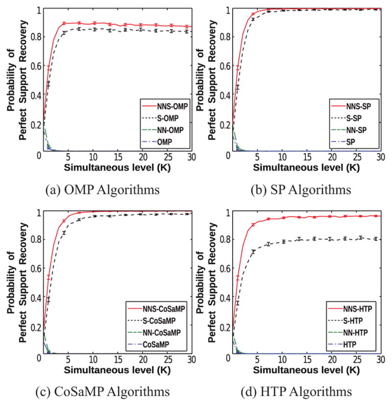
The simulations described in this subsection all use iid Gaussian Φ matrices, which are expected to have relatively good mutual coherence properties. Our first set of simulations explored the performance of the different greedy algorithms as a function of K, in a noiseless setting with M = 24, N = 128, p = 2, and fixed sparsity level S = 4. The simultaneous level K was systematically varied between 1 and 30. For each value of K, the simulation was repeated 5000 times with different realizations of X and Φ. Figure 1 shows the results of these simulations, plotting the perfect recovery probability as a function of K. We say that perfect recovery has occurred for a given problem realization whenever the infinity norm of the reconstruction error ||X − X̂||_∞ is less than 10⁻⁴. We estimate the probability of perfect recovery by taking ratio between the number of perfect recoveries and the total number of trials. The plots also include a 95% confidence interval for the probability of perfect recovery, which we computed using the Wald test [37]. The results indicate that algorithms that use NNS or SS constraints have better performance than algorithms that do not use any form of SS constraints, and that the performance gap increases as the simultaneous level K increases.⁴ This is not surprising, since the SS constraint provides valuable prior information that is not fully captured by NN or unstructured sparsity constraints. As expected, we also observe that the NNS algorithms outperform the algorithms based on SS constraints alone.

Figure 1.

The empirical probability of perfect recovery as a function of K for the noiseless first set of simulations. Results are plotted for SS X matrices drawn iid from (a)–(d) the Rayleigh distribution and (e)–(f) the Uniform [0, 1] distribution. Results are shown for (a,e) OMP-based algorithms, (b,f) SP-based algorithms, (c,g) CoSaMP-based algorithms, and (d,h) HTP-based algorithms. The error bars in each plot represent 95% confidence intervals.

While the perfect recovery probabilities were not identical for X matrices generated using the Rayleigh and Uniform probability densities, the general performance trends we observed were similar. This was also true for our other simulations, and for simplicity, we only show Rayleigh X in what follows.

Our second set of simulations explored the performance of our proposed algorithms in the presence of noise. Simulation parameters were identical to the first simulation, except that we fixed K = 8 and added noise with SNR values ranging from 0 dB to 100 dB. Since perfect recovery is generally not possible in the noisy case, we measured performance by estimating the probability of perfect support recovery. We say that perfect support recovery has occurred for a given problem realization if Λ̂_SS = Λ_SS (X). Plots of the perfect support recovery probability versus SNR are shown in Fig. 2. We observe that algorithm performance decreases rapidly at lower SNR values (< 60 dB) unless the algorithms use SS constraints. On the other hand, the NNS and SS algorithms still show good performance, with perfect support recovery probabilities higher than 0.75 for SS and higher than 0.9 for NNS when SNR = 10 dB. As in the noiseless case, the proposed NNS algorithms outperform the SS algorithms, sometimes substantially. These simulations demonstrate that the proposed algorithms can still perform well in the presence of substantial noise.

Figure 2.

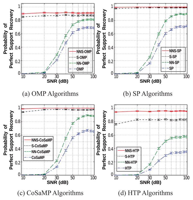
The empirical probability of perfect support recovery as a function of SNR (dB) for the second set of simulations with K = 8. The error bars in each plot represent 95% confidence intervals.

To further explore performance characteristics in the noisy setting, we performed a third set of simulations with SNR fixed at the relatively low value of 10 dB and allowing K to vary. All other parameters were identical to those of the previous simulations. Results are shown in Fig. 3, and again demonstrate the value of using both NN and SS constraints together. Our proposed NNS algorithms have better performance than the alternatives. The algorithms based on SS constraints perform comparably well for larger K for certain algorithms (e.g., Fig. 3(b)), though a substantial gap is still present for others (e.g., Fig. 3(d)).

Figure 3.

The empirical probability of perfect support recovery as a function of the simultaneous level K for the third set of simulations with SNR = 10 dB. The error bars in each plot represent 95% confidence intervals.

Our previous simulations explored algorithm performance for the relatively small sparsity level of S = 4. Our fourth and fifth simulations explore algorithm performance as a function of S. Both of these simulations used M = 64, N = 128, p = 2, and K = 8, with S systematically varied between 2 and 60. Each simulation was repeated 1000 times with different realizations of X, Φ, and N. The fourth simulation used noiseless data, with results shown in Fig. 4, while the fifth simulation used noisy data (SNR=30 dB and 10 dB), with results shown in Fig. 5. These figures demonstrate that the NNS algorithms still outperform the alternative approaches for larger values of S in both the noisy and noiseless cases. In the noiseless case, NNS-SP had surprisingly good performance, and was always able to perfectly recover signals with S ≤ 40, despite the fact that M = 60 is not very big relative to S = 40. In the noisy case, while the NNS-based approaches have performance advantages, it should be noted that this advantage is particularly strong at higher SNR, and that the gap between NNS performance and SS performance is smaller at SNR=10 dB.

Figure 4.

The empirical probability of perfect recovery as a function of the sparsity level S for the noiseless fourth set of simulations. The error bars in each plot represent 95% confidence intervals.

Figure 5.

The empirical probability of perfect support recovery as a function of the sparsity level S for the fifth set of simulations with noisy signal. (a)–(d) SNR = 30dB, (e)–(f) SNR = 10dB. The error bars in each plot represent 95% confidence intervals.

In addition to the recovery performance, we also evaluated the algorithms with respect to the number of iterations and total computation time. The computational complexity of each algorithm is difficult to analyze theoretically because the convergence characteristics and number of iterations for NNLS and many of the greedy algorithms are data dependent and hard to predict in advance. As a result, our computational comparisons are empirical. We simulated noiseless data with M = 24, N = 128, p = 2, and S = 4. We calculated the mean number of iterations until convergence for each algorithm based on 200 independent simulated datasets, and results are shown in Table 1. The table shows that the mean number of iterations was similar for all algorithms, generally ranging between 3 and 5 for this problem. However, the NNS algorithms had a slightly smaller mean number of iterations. We also measured the mean computation time for each algorithm based on 1000 independent simulated datasets, and results are plotted in Fig. 6. We observe that the NN constrained methods (red and green) frequently require more computation time than their non-NN counterparts. This can be partially attributed to the fact that solving the NNLS problem in (11) is being done iteratively, while the LLS problem in (6) is being solved noniteratively using simple matrix inversion. We also observe that the SS algorithms are generally faster than their non-SS counterparts. This can be partially attributed to the fact that the SS methods compute the columns of X̂ simultaneously, while our implementations of the non-SS methods compute each column of X̂ sequentially. As a result, our proposed NNS algorithms are generally not as fast as algorithms that do not impose NN constraints, though our proposed NNS algorithms are still generally faster than NN algorithms.

Table 1.

Mean iterations for different algorithms with S = 4

	Simultaneous level (K)
	5	10	15	20	25	30
SP	3.66	3.65	3.63	3.64	3.65	3.68
NN-SP	3.47	3.50	3.45	3.49	3.47	3.51
S-SP	3.29	3.20	3.15	3.20	3.25	3.21
NNS-SP	3.22	3.12	3.15	3.14	3.12	3.15
CoSaMP	4.52	4.60	4.55	4.56	4.57	4.57
NN-CoSaMP	3.43	3.43	3.40	3.41	3.40	3.44
S-CoSaMP	4.27	4.21	4.17	4.12	4.14	4.30
NNS-CoSaMP	3.17	3.14	3.19	3.20	3.16	3.21
HTP	4.78	4.73	4.73	4.73	4.75	4.73
NN-HTP	4.65	4.66	4.60	4.64	4.63	4.66
S-HTP	4.39	4.33	4.37	4.35	4.47	4.25
NNS-HTP	4.31	4.15	4.19	4.21	4.27	4.26

Note: The number of iterations for all OMP algorithms is S = 4.

Figure 6.

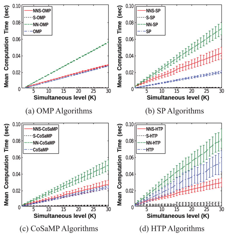
Mean computation time as a function of the simultaneous level K. The error bars in each plot represent standard deviations of the computation time.

6.2. Rayleigh Φ Matrices

We also evaluated the proposed NNS greedy algorithms using iid Rayleigh Φ matrices. Simulation parameters were otherwise identical to the first set of simulations from Section 6.1, with M = 24, N = 128, p = 2, and S = 4. The Rayleigh matrices are nonnegative matrices with much worse mutual coherences than iid Gaussian matrices, and are likely to benefit from the conditioning procedure described in Section 4.1. For example, we empirically compute the average mutual coherence of 24×128 iid Gaussian matrices as ≈ 0.708, while the average mutual coherence is ≈ 0.908 for the Rayleigh case.⁵ To show the effects of conditioning, we compared results obtained using the original linear models Y = ΦX against results obtained with the conditioned linear models CY = CΦX. For reference, the conditioned linear models empirically had an average mutual coherence of ≈ 0.811.

Figure 7 shows the noiseless recovery performance as a function of K. As expected, performance is substantially worse in this case relative to the iid Gaussian case when the conditioning procedure is not applied. In addition, the performance of the NNS greedy algorithms is not very different from the performance of SS greedy algorithms in the absence of conditioning, though the NNS and SS greedy algorithms still substantial outperform the greedy algorithms that only impose NN or unstructured sparsity. Our analysis suggests that the minimal difference between SS and NNS is related to the fact that that the Φ and Y are both NN in this case, leading to substantially more strong positive residual correlations relative to strong negative residual correlations. However, substantial performance improvements for all algorithms are obtained by applying the conditioning procedure, and as before, we observe substantial performance advantages for the NNS greedy algorithms relative to the alternative algorithms that impose less structure.

Figure 7.

The empirical probability of perfect recovery as a function of K for the simulations using Rayleigh matrices Φ. Results are plotted for SS X matrices estimated from (a)–(d) the original linear model Y = ΦX and (e)–(h) the conditioned linear model CY = CΦX. The entries of X were drawn iid from a Rayleigh distribution. Results are shown for (a,e) OMP-based algorithms, (b,f) SP-based algorithms, (c,g) CoSaMP-based algorithms, and (d,h) HTP-based algorithms. The error bars in each plot represent 95% confidence intervals.

7. Application Example

The previous sections evaluated our proposed methods in the context of simulated data. In this section, we demonstrate the potential benefits of our proposed algorithms in the context of a real-world magnetic resonance imaging (MRI) application. Specifically, we used greedy algorithms to estimate the orientation of fiber bundles from high angular resolution diffusion MRI (HARDI) data [38]. HARDI measurements provide information about the random (Brownian) thermal motion of water molecules in the body. This information can be used to infer fiber orientations, since water diffusion is generally anisotropic in fibrous structures, with a tendency for water to displace by longer distances along the principal axis of the fiber [39]. When applied to the human brain, the fiber orientation information can subsequently be used to identify the trajectories of neuronal fiber bundles (the “wires” that carry communications between different brain regions), which provide a form of “wiring diagram” that describes the physical backbone of the brain’s internal network.

Within the HARDI literature, an important class of orientation estimation methods models the observed signal as a sparse and nonnegative mixture of basis functions [40–42], where each basis function is a rotated and resampled version of the same basic function, and the prototype function corresponds to the ideal data that would be measured from an ideal fiber bundle. Once the measured data has been decomposed in this basis, the orientation distribution functions (ODFs) that describe the ensemble probability of water displacement along a given orientation can be obtained by applying appropriate transformations to each basis function. An example of several diffusion basis functions and corresponding ODFs is shown in Fig. 8.

Figure 8.

(Top Row) Example diffusion basis functions, which are all resampled rotations of the same basic prototype function. (Bottom Row) ODFs, computed using the Funk-Radon and Cosine Transform [51], corresponding to the diffusion basis functions from the top row. The locations of the largest maximum of each ODF indicate the primary orientations of the corresponding fiber bundle. The diffusion signals and the ODFs have been color-coded by orientation.

This section applies greedy algorithms to HARDI data with NNS constraints to obtain ODF estimates that reflect the following characteristics:

• The number of distinct fiber bundles that are present in small local region of brain tissue is typically assumed to be small (e.g., 1–3 fiber bundles per voxel [43]). A major benefit of greedy methods is that the sparsity level S can be specified manually, which allows this additional prior information to be injected into the estimation process.

• Fiber bundles are continuous and generally follow smooth paths through space, which means that fiber orientations are frequently consistent within small local spatial neighborhoods [44]. This implies that a SS model may be reasonable for certain brain regions.

• “Negative” fiber bundles are unphysical [40–42].

Our example uses Fiber Cup diffusion phantom data [45, 46] that was acquired using a diffusion encoding b-value of 2000 s/mm², M = 64 different measurement orientations, and 3 mm isotropic spatial resolution. The diffusion phantom consists of water-filled acrylic fiber bundles. We specifically examined a group of K = 128 voxels from a spatial region where two straight fiber bundles cross at an approximately 90° angle.

Orientation estimation from HARDI data was mapped into problem P_Ω as described below.

• The data matrix Y ∈ ℝ^M×K was constructed by reformatting the diffusion data from each of M = 64 measurement orientations and K = 128 spatial locations into an M × K matrix.

• The dictionary matrix Φ ∈ ℝ^M×N was obtained by rotating a prototype basis function along each of N=1296 orientations. The orientations were designed to be uniformly spaced on the sphere using an electrostatic repulsion model [47]. The prototype function was obtained by fitting a spherical harmonic model [48] to data from a spatial region containing a single fiber bundle.

• The unknown (to be estimated) matrix X ∈ ℝ^N×K contains the basis function coefficients, which we know in advance will be sparse and NN.

The matrix X̂ was estimated using the SP algorithms with sparsity level S = 2 from the conditioned linear model CY = CΦX, and the results are shown in Fig. 9. As shown in the figure, the proposed NNS-SP algorithm clearly depicts the known geometry of the phantom (two straight fiber bundles that cross at an approximately 90° angle). In contrast, the NN-SP algorithm yields a field of estimated ODFs that have substantial spatial variability and do not reproduce the known geometry as accurately. In addition, the standard SP and S-SP algorithms produce unphysical negative coefficients for certain voxels, which induces the appearance of unusually large ODFs. Results using OMP, CoSaMP, and HTP-based algorithms were similar, and are not shown. These results demonstrate the potential advantages of our proposed greedy NNS algorithms in real-world applications.

Figure 9.

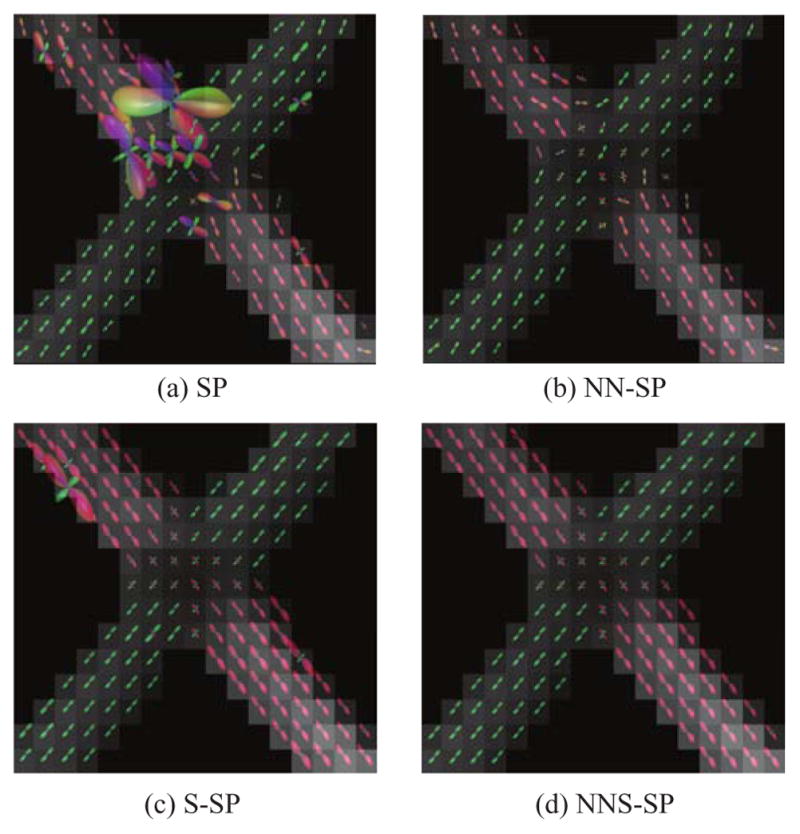
ODFs estimated using (a) standard SP, (b) NN-SP, (c) S-SP and (d) NNS-SP.

8. Discussion

It is worth emphasizing that, while Theorem 1 indicates that performance guarantees can exist for our proposed NNS algorithms, the theory that we have derived is almost completely inapplicable in any of the empirical results we have considered because of the large mutual coherences of the Φ matrices. Given the structure of most NNS inverse problems, we believe that this is likely to be a widespread occurrence in practical applications. However, we do not view the lack of strong theoretical guarantees as a barrier to the use of intelligently designed algorithms that demonstrate good empirical performance. For example, MRI reconstruction from undersampled data is often described as one of the prototypical “success stories” of sparse recovery theory and methods, despite the fact that the existing theoretical performance guarantees are largely inapplicable in these scenarios [49], which means that most good sparsity-based MRI reconstruction results should be considered heuristic rather than theoretically justified. However, whenever theoretical guarantees are absent in the context of a specific application, it is important to perform thorough application-specific testing of the algorithms to help ensure that the algorithms will generate desirable results.

Similar to existing greedy algorithms, many of our proposed algorithms depend on prior knowledge of S, which may not always be known in practice. Our preliminary experience indicates that our proposed NNS algorithms can still be very successful and still consistently outperform the less-constrained greedy algorithms in cases when S is overestimated, though a leave more detailed explorations to future work.

It is also worth mentioning that the use of a least-squares data fidelity criterion in P_Ω can be viewed as implicitly using a Gaussian noise model. However, for many applications where NN constraints are reasonable, the data might be more accurately described by the Rician distribution (i.e., each measured data sample is equal to the magnitude of a Gaussian random variable) or the non-central chi distribution (i.e., each measured data sample is equal to the square root of sum-of-squared magnitudes of multiple Gaussian random variables). It should be noted that P_Ω is still relevant to such cases. Specifically, we have recently introduced a quadratic majorize-minimize procedure [50] that allows Rician and noncentral chi log-likelihoods to be maximized by iteratively solving a sequence of NNLS problems, where each NNLS problem has the same form as P_Ω. This type of approach is easily adapted to our proposed NNS greedy algorithms.

9. Conclusions

This paper proposed a new family of NNS greedy algorithms, and showed empirically that such algorithms can be an effective way to recover NNS signals in ill-conditioned or underdetermined scenarios where the incorporation of accurate additional prior information will generally be expected to enhance reconstruction performance. While we have concentrated primarily on the empirical performance characteristics of these algorithms, we have also proven a performance guarantee for NNS-OMP under mutual coherence conditions on Φ, and conjecture that better theoretical performance guarantees for these algorithms can also be established. We expect that these algorithms and their extensions will prove useful in a wide variety of applications where NN and SS structure is reasonable to assume.

References

- 1.Davis G, Mallat S, Avellaneda M. Adaptive greedy approximations. Constr Approx. 1997;13:57–98. doi: 10.1007/BF02678430. [DOI] [Google Scholar]
- 2.Donoho DL, Elad M, Temlyakov VN. Stable recovery of sparse overcomplete representations in the presence of noise. IEEE Trans Inf Theory. 2006;52:6–18. doi: 10.1109/TIT.2005.860430. [DOI] [Google Scholar]
- 3.Tropp JA, Gilbert AC. Signal recovery from random measurements via orthogonal matching pursuit. IEEE Trans Inf Theory. 2007;53:4655–4666. doi: 10.1109/TIT.2007.909108. [DOI] [Google Scholar]
- 4.Cai TT, Wang L. Orthogonal matching pursuit for sparse signal recovery with noise. IEEE Trans Inf Theory. 2011;57:4680–4688. doi: 10.1109/TIT.2011.2146090. [DOI] [Google Scholar]
- 5.Dai W, Milenkovic O. Subspace pursuit for compressive sensing signal reconstruction. IEEE Trans Inf Theory. 2009;55:2230–2249. doi: 10.1109/TIT.2009.2016006. [DOI] [Google Scholar]
- 6.Needell D, Tropp JA. CoSaMP: Iterative signal recovery from incomplete and inaccurate samples. Appl Comput Harmon Anal. 2009;26:301–321. doi: 10.1145/1859204.1859229. [DOI] [Google Scholar]
- 7.Foucart S. Hard thresholding pursuit: An algorithm for compressive sensing. SIAM J Numer Anal. 2011;49:2543–2563. doi: 10.1137/100806278. [DOI] [Google Scholar]
- 8.Blumensath T, Davies ME. Normalized iterative hard thresholding: Guaranteed stability and performance. IEEE J Sel Topics Signal Process. 2010;4:298–309. doi: 10.1109/JSTSP.2010.2042411. [DOI] [Google Scholar]
- 9.Whittall KP, MacKay AL. Quantitative interpretation of NMR relaxation data. J Magn Reson. 1989;84:134–152. doi: 10.1016/0022-2364(89)90011-5. [DOI] [Google Scholar]
- 10.Kumar D, Nguyen TD, Gauthier SA, Raj A. Bayesian algorithm using spatial priors for multi-exponential T2 relaxometry from multiecho spin echo MRI. Magn Reson Med. 2012;68:1536–1543. doi: 10.1002/mrm.24170. [DOI] [PubMed] [Google Scholar]
- 11.Lin Y, Haldar JP, Li Q, Conti PS, Leahy RM. Sparsity constrained mixture modeling for the estimation of kinetic parameters in dynamic PET. IEEE Trans Med Imag. 2014;33:173–185. doi: 10.1109/TMI.2013.2283229. [DOI] [PMC free article] [PubMed] [Google Scholar]
- 12.Ma WK, Bioucas-Dias JM, Chan TH, Gillis N, Gader P, Plaza AJ, Ambikapathi A, Chi CY. A signal processing perspective on hyperspectral unmixing: Bridging the gap between remote sensing and signal processing. IEEE Signal Process Mag. 2014;31:67–81. doi: 10.1109/MSP.2013.2279731. [DOI] [Google Scholar]
- 13.Hoyer PO. Non-negative matrix factorization with sparseness constraints. J Mach Learn Res. 2004;5:1457–1469. [Google Scholar]
- 14.Donoho DL, Tanner J. Sparse nonnegative solution of underdetermined linear equations by linear programming. Proc Natl Acad Sci USA. 2005;102:9446–9451. doi: 10.1073/pnas.0502269102. [DOI] [PMC free article] [PubMed] [Google Scholar]
- 15.Bruckstein AM, Elad M, Zibulevsky M. On the uniqueness of nonnegative sparse solutions to underdetermined systems of equations. IEEE Trans Inf Theory. 2008;54:4813–4820. doi: 10.1109/TIT.2008.929920. [DOI] [Google Scholar]
- 16.Leviatan D, Temlyakov VN. Simultaneous approximation by greedy algorithms. Adv Comput Math. 2006;25:73–90. doi: 10.1007/s10444-004-7613-4. [DOI] [Google Scholar]
- 17.Cotter SF, Rao BD, Engan K, Kreutz-Delgado K. Sparse solutions to linear inverse problems with multiple measurement vectors. IEEE Trans Signal Process. 2005;53:2477–2488. doi: 10.1109/TSP.2005.849172. [DOI] [Google Scholar]
- 18.Chen J, Huo X. Theoretical results on sparse representations of multiple-measurement vectors. IEEE Trans Signal Process. 2006;54:4634–4643. doi: 10.1109/TSP.2006.881263. [DOI] [Google Scholar]
- 19.Tropp JA, Gilbert AC, Strauss MJ. Algorithms for simultaneous sparse approximation. Part I: Greedy pursuit. Signal Process. 2006;86:572–588. doi: 10.1016/j.sigpro.2005.05.030. [DOI] [Google Scholar]
- 20.Gribonval R, Rauhut H, Schnass K, Vandergheynst P. Atoms of all channels, unite! Average case analysis of multi-channel sparse recovery using greedy algorithms. J Fourier Anal Appl. 2008;14:655–687. doi: 10.1007/s00041-008-9044-y. [DOI] [Google Scholar]
- 21.Foucart S. Recovering jointly sparse vectors via hard thresholding pursuit. Proc SAMPTA. 2011 [Google Scholar]
- 22.Lee K, Bresler Y, Junge M. Subspace methods for joint sparse recovery. IEEE Trans Inf Theory. 2012;58:3613–3641. doi: 10.1109/TIT.2012.2189196. [DOI] [Google Scholar]
- 23.Davies ME, Eldar YC. Rank awareness in joint sparse recovery. IEEE Trans Inf Theory. 2012;58:1135–1146. doi: 10.1109/TIT.2011.2173722. [DOI] [Google Scholar]
- 24.Blanchard JD, Cermak M, Hanle D, Jing Y. Greedy algorithms for joint sparse recovery. IEEE Trans Signal Process. 2014;62:1694–1704. doi: 10.1109/TSP.2014.2301980. [DOI] [Google Scholar]
- 25.Chen D, Plemmons RJ. Nonnegativity constraints in numerical analysis. In: Bultheel A, Cools R, editors. The Birth of Numerical Analysis. World Scientific Publishing; 2010. pp. 109–139. [Google Scholar]
- 26.Wang M, Xu W, Tang A. A unique “nonnegative” solution to an underdetermined system: From vectors to matrices. IEEE Trans Signal Process. 2011;59:1007–1016. doi: 10.1109/TSP.2010.2089624. [DOI] [Google Scholar]
- 27.Meinshausen N. Sign-constrained least squares estimation for high-dimensional regression. Electron J Statist. 2013;7:1607–1631. doi: 10.1214/13-EJS818. [DOI] [Google Scholar]
- 28.Slawski M, Hein M. Non-negative least squares for high-dimensional linear models: Consistency and sparse recovery without regularization. Electron J Statist. 2013;7:3004–3056. doi: 10.1214/13-EJS868. [DOI] [Google Scholar]
- 29.Eldar YC, Kutyniok G, editors. Compressed Sensing: Theory and Applications. Cambridge University Press; 2012. [Google Scholar]
- 30.Duarte MF, Eldar YC. Structured compressed sensing: From theory to applications. IEEE Trans Signal Process. 2011;59:4053–4085. doi: 10.1109/TSP.2011.2161982. [DOI] [Google Scholar]
- 31.Lawson CL, Hanson RJ. Solving least squares problems. Vol. 15. SIAM; Philadelphia: 1995. [Google Scholar]
- 32.Tropp JA. Algorithms for simultaneous sparse approximation. Part II: Convex relaxation. Signal Process. 2006;86:589–602. doi: 10.1016/j.sigpro.2005.05.031. [DOI] [Google Scholar]
- 33.Yuan M, Lin Y. Model selection and estimation in regression with grouped variables. J R Stat Soc Ser B. 2006;68:49–67. doi: 10.1111/j.1467-9868.2005.00532.x. [DOI] [Google Scholar]
- 34.Fornasier M, Rauhut H. Recovery algorithms for vector-valued data with joint sparsity constraints. SIAM J Numer Anal. 2008;46:577–613. doi: 10.1137/0606668909. [DOI] [Google Scholar]
- 35.Chartrand R, Wohlberg B. A nonconvex ADMM algorithm for group sparsity with sparse groups. Proc IEEE Int Conf Acoust, Speech, Signal Process. 2013:6009–6013. doi: 10.1109/ICASSP.2013.6638818. [DOI] [Google Scholar]
- 36.Haldar JP, Hernando D. Rank-constrained solutions to linear matrix equations using Power Factorization. IEEE Signal Process Lett. 2009;16:584–587. doi: 10.1109/LSP.2009.2018223. [DOI] [PMC free article] [PubMed] [Google Scholar]
- 37.Harrell FE. Regression modeling strategies: with applications to linear models, logistic regression, and survival analysis. Springer; New York: 2001. [Google Scholar]
- 38.Tuch DS, Reese TG, Wiegell MR, Makris N, Belliveau JW, Wedeen VJ. High angular resolution diffusion imaging reveals intravoxel white matter fiber heterogeneity. Magn Reson Med. 2002;48:577–582. doi: 10.1002/mrm.10268. [DOI] [PubMed] [Google Scholar]
- 39.LeBihan D, Johansen-Berg H. Diffusion MRI at 25 exploring brain tissue structure and function. NeuroImage. 2012;61:324–341. doi: 10.1016/j.neuroimage.2011.11.006. [DOI] [PMC free article] [PubMed] [Google Scholar]
- 40.Ramirez-Manzanares A, Rivera M, Vemuri BC, Carney P, Mareci T. Diffusion basis functions decomposition for estimating white matter intravoxel fiber geometry. IEEE Trans Med Imag. 2007;26:1091–1102. doi: 10.1109/TMI.2007.900461. [DOI] [PubMed] [Google Scholar]
- 41.Wang Y, Wang Q, Haldar JP, Yeh FC, Xie M, Sun P, Tu TW, Trinkaus K, Klein RS, Cross AH, Song SK. Quantification of increased cellularity during inflammatory demyelination. Brain. 2011;134:3587–3598. doi: 10.1093/brain/awr307. [DOI] [PMC free article] [PubMed] [Google Scholar]
- 42.Cheng J, Deriche R, Jiang T, Shen D, Yap PT. Non-negative spherical deconvolution (NNSD) for estimation of fiber orientation distribution function in single-/multi-shell disffusion MRI. NeuroImage. 2014;101:750–764. doi: 10.1016/j.neuroimage.2014.07.062. [DOI] [PMC free article] [PubMed] [Google Scholar]
- 43.Jeurissen B, Leemans A, Tournier JD, Jones DK, Sijbers J. Investigating the prevalence of complex fiber configurations in white matter tissue with diffusion magnetic resonance imaging. Hum Brain Mapp. 2013;34:2747–2766. doi: 10.1002/hbm.22099. [DOI] [PMC free article] [PubMed] [Google Scholar]
- 44.Raj A, Hess C, Mukherjee P. Spatial HARDI: Improved visualization of complex white matter architecture with Bayesian spatial regularization. NeuroImage. 2011;54:396–409. doi: 10.1016/j.neuroimage.2010.07.040. [DOI] [PMC free article] [PubMed] [Google Scholar]
- 45.Fillard P, Descoteaux M, Goh A, Gouttard S, Jeurissen B, Malcolm J, Ramirez-Manzanares A, Reisert M, Sakaie K, Tensaouti F, Yo T, Mangin JF, Poupon C. Quantitative evaluation of 10 tractography algorithms on a realistic diffusion MR phantom. NeuroImage. 2011;56:220–234. doi: 10.1016/j.neuroimage.2011.01.032. [DOI] [PubMed] [Google Scholar]
- 46.Poupon C, Rieul B, Kezele I, Perrin M, Poupon F, Mangin JF. New diffusion phantom dedicated to the study and validation of high-angular-resolution diffusion imaging (HARDI) models. Magn Reson Med. 2008;60:1276–1283. doi: 10.1002/mrm.21789. [DOI] [PubMed] [Google Scholar]
- 47.Jones DK, Horsfield MA, Simmons A. Optimal strategies for measuring diffusion in anisotropic systems by magnetic resonance imaging. Magn Reson Med. 1999;42:515–525. doi: 10.1002/(SICI)1522-2594(199909)42:3<515::AID-MRM14>3.0.CO;2-Q. [DOI] [PubMed] [Google Scholar]
- 48.Descoteaux M, Angelino E, Fitzgibbons S, Deriche R. Regularized, fast, and robust analytical Q-ball imaging. Magn Reson Med. 2007;58:497–510. doi: 10.1002/mrm.21277. [DOI] [PubMed] [Google Scholar]
- 49.Haldar JP, Hernando D, Liang ZP. Compressed-sensing MRI with random encoding. IEEE Trans Med Imag. 2011;31:893–903. doi: 10.1109/TMI.2010.2085084. [DOI] [PMC free article] [PubMed] [Google Scholar]
- 50.Varadarajan D, Haldar JP. A majorize-minimize framework for Rician and non-central chi MR images. IEEE Trans Med Imag. 2015;24:2191–2202. doi: 10.1109/TMI.2015.2427157. [DOI] [PMC free article] [PubMed] [Google Scholar]
- 51.Haldar JP, Leahy RM. Linear transformations for Fourier data on the sphere: Application to high angular resolution diffusion MRI of the brain. NeuroImage. 2013;72:233–247. doi: 10.1016/j.neuroimage.2013.01.022. [DOI] [PMC free article] [PubMed] [Google Scholar]
Associated Data
This section collects any data citations, data availability statements, or supplementary materials included in this article.