DISCRIMINATION OF SCHIZOPHRENIA AUDITORY HALLUCINATORS BY MACHINE LEARNING OF RESTING-STATE FUNCTIONAL MRI

Abstract

Auditory hallucinations (AH) are a symptom that is most often associated with schizophrenia, but patients with other neuropsychiatric conditions, and even a small percentage of healthy individuals, may also experience AH. Elucidating the neural mechanisms underlying AH in schizophrenia may offer insight into the pathophysiology associated with AH more broadly across multiple neuropsychiatric disease conditions. In this paper, we address the problem of classifying schizophrenia patients with and without a history of AH, and healthy control subjects. To this end, we performed feature extraction from resting state functional magnetic resonance imaging (rsfMRI) data and applied machine learning classifiers, testing two kinds of neuroimaging features: (a) functional connectivity measures computed by lattice auto-associative memories (LAAM), and (b) local activity measures, including regional homogeneity (ReHo) and fractional amplitude of low frequency fluctuations (fALFF). We show that it is possible to perform classification within each pair of subject groups with high accuracy. Discrimination between patients with and without lifetime AH was highest, while discrimination between schizophrenia patients and healthy control participants was worst, suggesting that classification according to the symptom dimension of AH may be more valid than discrimination on the basis of traditional diagnostic categories. Functional connectivity measures seeded in right Heschl’s gyrus consistently showed stronger discriminative power than those seeded in left Heschl’s gyrus, a finding that appears to support AH models focusing on right hemisphere abnormalities. The cortical brain localizations derived from the features with strong classification performance are consistent with proposed AH models, and include left inferior frontal gyrus, parahippocampal gyri, the cingulate cortex, as well as several temporal and prefrontal cortical brain regions. Overall, the observed findings suggest that computational intelligence approaches can provide robust tools for uncovering subtleties in complex neuroimaging data, and have the potential to advance the search for more neuroscience-based criteria for classifying mental illness in psychiatry research.

1. Introduction

Auditory hallucinations (AH) are auditory perceptions in the absence of external acoustical stimuli^{3; 59}. They are a common symptom in schizophrenia, but they can be present in other psychiatric disorders, in neurological conditions, such as epilepsy³³, in states of drug intoxication or withdrawal, and even in 10–15% of healthy subjects^{85; 89}. The pathophysiology underlying AH may be shared to some degree across multiple disease conditions. Thus, elucidating the neural mechanisms underlying AH in schizophrenia may offer insight into the mechanisms associated with AH more broadly.

Several models of AH pathogenesis have been proposed ^{3; 36; 40; 63; 59; 65; 71; 83; 95}, but the exact pathophysiology remains unclear. According to inner speech theories, AH occur when inner speech is misattributed as originating outside the self. Source monitoring accounts focus on preconscious top-down cognitive processes such as the influence of cues, personal beliefs, and expectations in the failure to recognize “self” attributes of inner speech^{41; 17; 91}. Feed forward models, which provide a more bottom-up explanatory framework, propose that AH result from a breakdown in corollary discharge, a system that signals via an “efference copy” that a particular motor output is about to be produced^{20; 21}. In the case of inner speech, discharges from motor speech production areas fail to inhibit speech perception areas, and the self-produced speech is thus perceived as coming from an external source²³. Studies investigating such feed forward models tend to focus on structural and functional disconnection between the frontal and temporoparietal areas^{3; 59; 81; 84}. Models based in signal detection theory⁵ suggest that AH result from greater perceptual bias to detect auditory signals, especially signals consisting of personally salient words¹⁸. A memory-based model proposes that AH are unintentionally activated auditory representations from memory which have been dissociated from their original context⁹⁴. A more neuroanatomically oriented model proposes that AH arise from heightened bottom-up activity in the left STG priming the brain for “over-perceptualization,” combined with a failure of top-down control from the anterior cingulate, prefrontal, premotor, and cerebellar cortices leading to a breakdown in monitoring³. A similar model suggests it is the failure of prefrontal executive functions to inhibit activity in the STG (the perceptual origin of AH) and parietal cortex (the purported center of attention to the voice), due to frontotemporoparietal disconnection, that leads to AH³⁶. Still another hypothesis, focusing on network connectivity⁶⁴, suggests that abnormal interaction between the default mode network and the auditory cortex at rest is the fundamental mechanism leading to AH. Most of these models are not mutually exclusive, and there are ongoing efforts to integrate such models into a more unified view⁹⁵.

Studies on the neural substrates associated with AH pathophysiology, as proposed in the above and other AH models, have utilized a wide range of neuroimaging techniques³. These include volumetric and morphometric magnetic resonance imaging (MRI) studies^{48; 71}, diffusion tensor imaging (DTI) to assess white matter integrity¹⁴, functional activation studies using positron emission tomography (PET) or functional MRI (fMRI)⁸⁶, and functional connectivity studies^{16; 40; 51; 52} using resting-state fMRI (rsfMRI)^{24; 76}. RsfMRI enables the study of correlations between low frequency components of voxel time series⁷, which are proposed to reflect intrinsic functional correlations between brain regions^{7; 101}. RsfMRI data are aquired in awake subjects in a passive mind state; because rsfMRI does not impose on the cognitive abilities of the subjects, it can be performed with a wide variety of subjects and cognitive conditions. RsfMRI has been used to study brain development¹⁹, depression ^{100; 31}, Alzheimer’s Disease ⁵⁵, and schizophrenia^{61; 70; 96; 105; 106}.

RsfMRI studies of schizophrenia patients with AH have used varying methods and asked different questions about AH-related connectivity^{25; 84; 81; 92; 80; 97; 34; 54; 11; 68}. A recent study by members of our group⁸¹ investigated differences between schizophrenia patients with and without a history of AH in the resting state network correlating with voxels in left Heschl’s gyrus (LHG) (MNI coordinates −42,–26,10), the location of the primary auditory cortex in humans¹³. The LHG seed was selected because it has been identified in anatomical^{71; 62} and functional studies¹⁶ as important in AH pathogenesis. We found that LHG functional connectivity (FC) to classical Broca’s territory in inferior frontal gyrus, dorsal anterior cingulate cortex (dACC), and other frontotemporal regions is elevated in AH and covaries with AH severity. In contrast to the results from the symptom covariate analysis, the findings from the group-wise comparisons were less robust.

Machine learning^{2; 82}, which is a branch of artificial intelligence, provides new ways to analyze neuroimaging data^{50; 102} and may offer advantages over traditional statistical inference approaches (for details, see section 3.1 describing the rationale for the approach). In machine learning models, dependent variables can be predicted on the basis of features extracted from the data. The feature extraction process, involving voxel saliency measures, can provide imaging biomarkers for the phenomena under study when the discriminant values can be mapped onto anatomical locations. Classification performance, as measured by accuracy and other indices, then enables assessment of a model’s predictive power. A variety of computational intelligence approaches have previously been applied to rsfMRI data analysis. These include artificial neural networks ⁵⁷, multivariate pattern analysis (MVPA)^{19; 72}, and a spiking neural network⁹⁸.

In this paper, we apply a novel lattice computing-based machine learning approach ^{27; 29; 30} to measure the accuracy with which rsfMRI data from schizophrenia patients with a history of AH (SZAH) can be discriminated from that of schizophrenia patients without a history of AH (SZ-NAH) and healthy controls (HC). In mathematics, a lattice is a partially ordered set in which every set of two elements has a join (or least upper bound) and a meet (or greatest lower bound)⁶. Inspired by mathematical morphology, lattice computing^{29; 45; 44} provides a non-linear approach to computational problem solving. In general terms, algorithms are built on lattice algebra [(ℝⁿ, ∧, ∨, +) where ∧ and ∨ are the minimum and maximum binary operators], instead of conventional linear algebra (ℝⁿ, +, ×)⁷⁸. Lattice computing provides numerically robust solutions, avoiding the problem of inverse computations which are inherent in linear approaches. Lattice computing is also faster than linear approaches because multiplications are replaced by additions in the construction of algorithms.

Auto-associative memories are intended to store patterns and to retrieve them from noisy or missing data. Linear auto-associative memories are single-layer networks made of interconnected linear units that operate in parallel⁴⁷. Because the representation of individual stimuli is not localized in the memory but distributed throughout the entire network, an auto-associative memory is able to retrieve an entire pattern of information given only partial or degraded versions of these stimuli; because of this property, auto-associative memories are often used in pattern recognition algorithms and for modeling human perceptual learning and memory¹. Lattice auto-associative memories (LAAM’s)^{77; 79} are built by replacing the linear algebraic functions of linear auto-associative memories with those of lattice algebra. In algorithms using auto-associative memories, recall error is the distance between the expected and actual recall patterns. With LAAM’s, the distance between the recalled input and the actual input may be used as a non-linear measure of similarity, which may be used as an alternative to correlation measures in functional connectivity analysis. LAAM’s show perfect recall of vectors whose elements are real numbers. In addition, because LAAM’s can recover stored patterns from even heavily distorted information, they are robust to specific types of noise. Because of this latter property, the distance between the recalled input and the actual input may be used as a non-linear measure of similarity, which may be used as an alternative to correlation measures in functional connectivity analysis. While methods involving LAAM-based distance cannot be expected to reproduce exactly the findings of methods using Pearson’s correlation coefficient, the LAAM findings may provide a complementary view of the data.

Besides LAAM-based FC, there are other features that can be extracted from rsfMRI data. Local activity measures include regional homogeneity (ReHo), which measures the correlation between the fMRI time series of a voxel and that of neighboring voxels¹⁰⁴; and the amplitude of low frequency fluctuations (ALFF) and fractional amplitude of low frequency fluctuations (fALFF)¹⁰⁷, which measure the strength of low frequency oscillations (LFOs) of the fMRI time series. ReHo and fALFF provide information about regional homogeneity and activation magnitude, respectively, and can offer insights that are complementary to information about FC.

Here, using LAAM-based FC to assess LHG connectivity with spatially distributed brain regions, and ReHo and fALFF to assess local activity, we demonstrate high accuracy, sensitivity, and specificity in discriminating SZAH from SZNAH and HC. To our knowledge, this is the first study to apply machine learning techniques, especially a novel lattice-based functional connectivity algorithm, to the classification of schizophrenia patients with and without AH.

2. Materials

We performed computational experiments on rsfMRI data from 68 men and women, ages 18–65 years, divided in three groups: (i) 26 schizophrenia patients (14 schizophrenia, 12 schizoaffective disorder, 1 schizophreniform disorder) with a history of AH (SZAH), (ii) 14 schizophrenia patients (5 schizophrenia, 8 schizoaffective disorder, and 1 schizophreni-form disorder) without a history of AH (SZNAH), and (iii) 28 healthy control subjects (HC). Data from one SZAH subject in the original dataset did not meet the current experiment’s criteria for angular head motion less than 3° and were thus not included. The Structured Clinical Interview for DSM-IV-TR (SCID)²² was administered to confirm axis I diagnosis in patients and to rule out major psychiatric illness in healthy control subjects. Item B16 of the SCID (“Did you ever hear things that other people couldn’t, such as noises, or the voices of people whispering or talking?”) was used to categorize patients into the SZAH and SZNAH groups; patients scoring threshold/true on B16 were coded SZAH, and all others SZNAH. AH severity was assessed with the psychotic symptom rating scale, AH subscale (PSYRATS-AH)³². Subjects were additionally interviewed post-scan about the presence of AH during image acquisition. PSYRATS-AH and post-scan de-briefing interviews were not completed in n=7 SZ-NAH patients whose data were acquired as part of a different dataset. Nearly all (n = 24/26) SZAH patients experienced verbal AH, as confirmed during the research interview and/or documented in the patients’ medical records; verbal AH could not be confirmed in two SZAH patients whose imaging data were originally acquired as part of a different dataset. For each subject we acquired 240 blood oxygen level dependent (BOLD) volumes and one T1-weighted anatomical image. Detailed participant characteristics (e.g., age, gender, handedness, illness duration, medication profiles) and image acquisition parameters are provided in the previous paper ⁸¹.

3. Methods

Our machine learning pipeline involved multiple steps, which are summarized in Figure 1 for the specific lattice computing based feature extraction approach. Briefly, they are: (1) Preprocessing. (2) Dimensionality reduction, which involved mapping the multivariate information (BOLD time series) of each voxel into a scalar measure of activity or connectivity (LAAM-based FC, ReHO, and fALFF). (3) Feature selection, which involved computing for each voxel site its saliency as the Pearson’s correlation coefficient (r) between two vectors, the first is composed the class labels of all the subjects, the second is composed of the voxel value of the scalar measure of activity or connectivity across all subjects. (4) We select the n voxel sites with greatest absolute r, instead of computing some threshold on the empirical distribution of the absolute r. We performed the classification experiments for the between-group comparisons of SZAH vs. SZNAH and SZAH vs. HC. For comparison, we also looked at classification performance for SZNAH vs. HC and SZ vs. HC. For each two-class classification problem, the feature selection process provides brain region localizations that may provide insights about AH pathophysiology. We provide more details for each of these steps below.

Fig. 1.

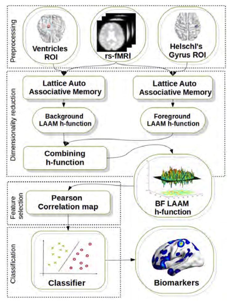
Analysis pipeline for the background/foreground (BF)-lattice auto associative memory (LAAM)-based functional connectivity approach. (1) RsfMRI data were preprocessed, and time series extracted from the specific background (CSF) and foreground (right or left Heschl’s gyrus) regions of interest. (2) We then performed dimensionality reduction, reducing the high dimensionality time series data into LAAM-based functional connectivity measures. (3) We performed feature selection and extraction, using the Pearson’s correlation coefficient (r) between the voxel value across subjects and the class label as a saliency measure to select the voxel sites with the greatest discriminative power. (4) We performed classification using support vector machines (SVM), and generate spatial maps showing the voxel sites with the features that are most highly discriminative.

3.1. Rationale for the approach

Before we present the details of the computational procedures, we will give an overall justification of the approach applied, signaling the points of departure from traditional inference-based approaches. Traditionally, in brain imaging, statistical inference approaches are used to detect significant differences between data from different populations, such as in voxel based morphometry (VBM) or analysis of fMRI task based data. The process is similar to alarm raising, failure detection, or target detection, which represent outlier detection problems, i.e., involving identification of items that do not comply with the input data distribution and fall outside the expected pattern. In this traditional approach, the problem is stated at the voxel level. The decision about whether to reject the null hypothesis (of no difference between groups) is made at each voxel independently. When the null hypothesis model is well known, the problem at each voxel is thereby reduced to the computation of a single threshold. When the number of tests is large, correction for multiple comparisons avoids false positives due to randomness. However, multiple comparisons corrections may also limit detection of real signal by increasing the risk of false negatives, or type II error.

Machine learning, by contrast, offers a more holistic approach, whereby the aim is to make a decision about the subject as an entity, i.e. is the person diseased or not? This approach places less importance on whether a statistically significant difference exists at any particular voxel. Rather than attributing to any voxel the credit for the decision, the goal of data processing is to extract informative features that contribute to the overall classification performance. In the current experiment, we are also interested in being able to identify localization information. Therefore, we look for features that map onto voxel sites that carry some anatomical meaning. This condition provides natural constraints to feature selection, and we select voxel sites on the basis of measures that are most salient in making a holistic decision about the subject. In such a process of feature selection, threshold based decisions and multiple comparisons correction algorithms do not apply.

Finally, we must take into account that fMRI data, which consist of time series, are characterized by high-dimensionality of information at each voxel. For computation of the significance measure it is necessary to reduce such data to a low-dimensional representation, e.g., a scalar value. To this end, we computed functional connectivity measures and local activity measures at each voxel. For functional connectivity we applied a novel lattice computing approach. The impetus for an alternative connectivity measure arose from the relative lack of robust group-wise connectivity results found by conventional linear correlation in our previous work⁸¹. As we already touch upon in the introduction, lattice auto-associative memories (LAAM’s) can serve as a non-linear measure of connectivity. The construction of LAAM’s is equivalent to the process of embedding data within a simplex (m-simplex is the convex hull of m + 1 affine independent points, which are the the vertices of the simplex; in this way, a 1-simplex is a line segment, a 2-simplex is a triangle and a 3-simplex is a tetrahedron, etc.)⁷⁸; so that transformations are naturally bounded and projected into the simplex boundaries. Because of their unique geometric architecture, LAAM’s: (1) remove the effect of data outliers that can give rise to undesired connectivity^{28; 10}, (2) are robust to specific dilative and erosive types of noise to which fMRI data are vulnerable^{75; 77; 79}, and (3) contain maximally discriminant information within the convex transformations of the data ³⁰. While we do not expect LAAM-based functional connectivity to reproduce exactly the findings of methods using Pearson’s correlation coefficient, the LAAM-based findings may provide an alternative and complementary view of the data. In addition to LAAM-based functional connectivity, we also extract local activity features, which measure the activity at a voxel or regional level. We expect that these local measures may reveal discriminant spatial distribution of the neural activity between populations.

3.2. Preprocessing

Data preprocessing began with skull removal using the brain extraction tool (BET) from FSL (http://www.fmrib.ox.ac.uk/fsl/). Images were manually oriented to the AC-PC line. The functional images were coregistered to the T1-weighted anatomical image. Using the Data Processing Assistant for Resting-State fMRI (DPARSF) (http://www.restfmri.net/forum/DPARSF) software package, the functional images were slice timing corrected, motion corrected (using a least squares approach and a 6-parameter spatial transformation), smoothed (FWHM=4mm), spatially normalized to the Montreal Neurological Institute (MNI) template (resampling voxel size = 3 mm × 3 mm × 3 mm), temporally band pass filtered (0.01–0.08 Hz) to remove very low frequency physiological noise and high frequency noise from non-neurological sources, and removed of linear trends. Mean BOLD time courses for head motion, global brain signal, white matter, and cerebrospinal fluid were regressed out before functional connectivity analysis. All the subjects had less than 3mm maximum displacement and less than 3° of angular motion.

3.3. Dimensionality reduction

Each voxel contains fMRI time series data, which have high-dimensionality. Prior to feature selection and extraction, the data need to be reduced to a low-dimensional representation, e.g., a scalar value. To this end, we computed functional connectivity measures and local activity measures at each voxel.

3.3.1. Functional connectivity measures derived from lattice auto-associative memories (LAAM’s)

Conventionally, FC is calculated as the time course correlation between a target ROI and other brain voxels. By contrast, in a lattice computing approach to FC, fMRI time series are stored as lattice auto-associative memories (LAAM’s), and FC is defined as the recall error, which is the distance between the expected and actual recall pattern when presenting the input to the memory.

Given a set of input/output pairs of real valued patterns $(X,Y)={\{({\mathbf{x}}^{\xi },{\mathbf{y}}^{\xi })\}}_{\xi =1}^k$, Lattice Hetero-Associative Memories (LHAM) are the morphological counterpart of the linear associative memories, defined by exchanging the conventional multiplication and addition operators by minimum/maximum and addition operators, respectively, i.e. defining the dual lattice dilative and erosive matrix multiplications and . Two dual constructions of LHAMs were originally proposed in ^{77; 79}: erosive LAM $W_{XY}={\bigwedge }_{\xi =1}^k\left[{\mathbf{y}}^{\xi }\times {(-{\mathbf{x}}^{\xi })}^{\prime }\right]$, and dilative LAM $M_{XY}={\bigvee }_{\xi =1}^k\left[{\mathbf{y}}^{\xi }\times {(-{\mathbf{x}}^{\xi })}^{\prime }\right]$. In these expressions, operator × can be any of the or operators, since y^ξ (−x^ξ)′ = y^ξ (−x^ξ)′. A special case of LHAM happens when X = Y, then W_XX and M_XX; this is called Lattice Auto-Associative Memories (LAAM). LAAMs have been applied to hyperspectral endmember induction²⁹, brain fMRI data segmentation³⁰, and pattern classification based on the LAAM’s recall error measured by the Chebyshev distance⁸⁷. Given dilative LAAM M_XX, the recall of input of vector x is ${\mathbf{x}}_M^{\#}=M_{XX}⍓\mathbf{x}$, and the recall error measured by the Chebyshev’s distance:

$$h_X(\mathbf{x})=d_C({\mathbf{x}}^{\#},\mathbf{x}),$$ (1)

where $d_C(\mathbf{a},\mathbf{b})={\bigvee }_{i=1}^n\mid a_i-b_i\mid$, is the Chebyshev distance between two vectors. Function h_X (x), which is the one-sided (OS)-LAAM h-function, can be used as a projection function from the high dimensional pattern space to a scalar magnitude. The erosive memory W_XX recall, i.e. ${\mathbf{x}}_W^{\#}=W_{XX}⍌\mathbf{x}$, could be used alternatively.

A Background/Foreground (BF) LAAM h-function is constructed by two OS-LAAM h-functions h_B and h_F, induced by dilative LAAMs M_BB and M_FF constructed on different training sets, i.e. background B and foreground F, respectively. We define the BF-LAAM h-function h_r (x) combining both h_B and h_F as follows:

$$h_r(\mathbf{x})=h_F(\mathbf{x})-h_B(\mathbf{x}),$$ (2)

which is positive for x ∈ ℱ (B), and negative for x ∈ ℱ (F), where ℱ (X) is the set of fixed points of M_XX. Therefore, h_r (x) is a discriminant function such that h_r (x) > 0 corresponds to data samples in the background class, and h_r (x) < 0 to data samples in the foreground class. The decision boundary is such that h_r (x) = 0.

When dealing with fMRI data, the training datasets correspond to brain ROI time-series. Computing either the one-sided or the BF-LAAM h-function for each voxel in an fMRI volume produces a scalar valued 3D h-map over the brain volume, which is a measure of the functional connectivity with this ROI used as the basis for feature selection and extraction for classification.

Here, we performed connectivity analysis to find the functional networks connected to the left (LHG) and right Heschl’s gyrus (RHG) (Figure 2) for each subject, following previous statistical inference works on correlation based FC⁸¹. We computed the OS-LAAM h-function, for which the training dataset X are the fMRI time series in the selected ROI. We also computed the BF-LAAM h-function, where the background training dataset B corresponds to the cerebrospinal fluid (CSF) ROI extracted from the brain ventricle voxels (MNI coordinates −15, −26,10), and the Foreground training dataset F is the average time signal from a selection of voxels in the LHG or the RHG (MNI coordinates 46, −20,8)⁸¹.

Fig. 2.

The ROIs used for lattice auto-associative memory (LAAM) based connectivity analysis. The fMRI time series from left Heschl’s gyrus (LHG; 10mm, MNI coordinates [−42, −26,10]) (a) and right Heschl’s gyrus (RHG; 10mm, MNI coordinates [46, −20, 8]) (b) were used to compute the left and right one-sided (OS)-LAAM h-functions, respectively. We also computed the background/foreground (BF)-LAAM h-functions, where the fMRI time series from the cerebrospinal fluid (CSF; 10mm, MNI coordinates [−15, −26, 10]) (c) was set as the background training dataset and the fMRI time series from the LHG (a) or RHG (b) were set as the foreground training dataset.

3.3.2. Local fMRI activity measures

We also computed local fMRI activity measures, which correspond to values measuring local properties of the signal:

1. Regional homogeneity (ReHo) is a local measure of the homogeneity of brain activity which computes the Kendall’s Coefficient of Concordance (W) between the time series of a given voxel and its nearest neighbors¹⁰⁴. Given a collection of vectors ${\{{\mathbf{x}}_j\in {ℝ}^n\}}_{j=1}^k$, which in our study correspond to voxel time series, the Kendall’s Coefficient of Concordance⁴⁶ is computed as follows:

   $$W=\frac{{\sum }_i{(R_i)}^2-n{(\overline{R})}^2}{\frac{1}{12}{k}^2(n^3-n)},$$ (3)

   where $R_i={\sum }_{j=1}^k{r}_{ij}$, and r_ij is the rank of the i-th time point in the j-th voxel. The value of W ranges from 0 to 1. R̄ = (n + 1) k/2 is the mean of the R_i. In our study W is used as a measure of the homogeneity of the neighborhood of a voxel in the Regional homogeneity (ReHo) measure. We apply a conventional 3D neighborhood, which is a 3D window around the voxel of dimensions 3×3×3 mm³. The W values are standardized and smoothed (4mm FWHM) to build a voxel-based scalar map for each subject.

2. Amplitude of low frequency fluctuations (ALFF)¹⁰³ and fractional amplitude of low frequency fluctuations (fALFF) ¹⁰⁷ are measures of the strength of low frequency oscillations (LFOs) of the BOLD signal. ALFF is defined as the total power within the frequency range between 0.01 and 0.1 Hz. fALFF is the relative contribution of specific LFO to the power of whole frequency range, defined as the power within the low-frequency range (0.01–0.1 Hz) split by the total power in the entire detectable frequency range ¹⁰⁸. In the current paper, we focus on fALFF.

3.4. Feature Selection and Extraction

Feature extraction gathers the values of the most salient voxels into a feature vector, used for classification. For this step, we computed the voxel saliency map. That is, for each voxel site, we computed the Pearson’s Correlation Coefficient (r) between its vector of values of the scalar feature across subjects with the class label categorical variable.

The Pearson’s Correlation Coefficient (r) is a measure of the linear correlation between two random variables samples given by vectors x, y ∈ ℝⁿ, it is computed as follows:

$$r=\frac{n({\sum }_i{x}_i{y}_i)-({\sum }_i{x}_i)({\sum }_i{y}_i)}{\sqrt{\left[n{\sum }_i{x}_i^2-{({\sum }_i{x}_i)}^2\right]\left[n{\sum }_i{y}_i^2-{({\sum }_i{y}_i)}^2\right]}},$$ (4)

so that r ∈ [−1, 1], r = 1 means that two variables have total positive correlation, and r = −1 means that they have total negative correlation, and r = 0 that there is no correlation at all. We use r between the voxel value across subjects and the class label variable as a saliency measure to select the voxel sites with the greatest discriminative power. Voxel sites with near zero r are not informative and can be discarded. Both positive or negative r values mean that the voxel site value can be an informative feature for classification.

Each classification experiment involves a separate saliency map, that is one per each scalar feature map and classification problem: We have explored the discrimination between each possible pair of classes: SZAH versus SZNAH, SZAH versus HC, SZNAH versus HC, and HC versus schizophrenia.

Feature selection looks for the n voxel sites with the largest absolute r values. Experiments are performed considering the following feature vector sizes: n = 500, 1000, 5000, 10000. Figures 3 and 4 show the regional localizations corresponding to feature vector dimension 1000 for the voxel saliency 3-dimensional maps obtained from OS LAAM h-function, BF LAAM h-function, and correlation based functional connectivity computed using either LHG or RHG ROIs, respectively. The brain regions were identified using the Harvard Oxford cortical atlas via the atlas query tool in FSL (http://www.fmrib.ox.ac.uk/fsl/). We show the localization results for the 1000 feature vector dimension because classification results across feature vector dimensions are similar, and the clusters in the 1000 dimension experiments are larger and thus easier to visualize.

Fig. 3.

Localization of feature voxel sites selected from the BF-LAAM h-function map with foreground seed extracted from the LHG ROI, when discriminating SZAH from SZnAH populations. Colorbar is proportional to voxel saliency.

Fig. 4.

Localization of feature voxel sites selected from the BF-LAAM h-function map with foreground seed extracted from the RHG ROI, when discriminating SZAH from SZnAH populations. Colorbar is proportional to voxel saliency.

Feature extraction builds the actual feature vectors extracting the selected voxel site values from the scalar feature map of each subject. Therefore, we have separate feature datasets for each classification experiment, scalar feature (i.e. FC, and local activity measures), and feature vector size.

3.5. Classification by Support Vector Machines (SVM)

Support Vector Machines (SVM)^{8; 90; 53} have become the de facto standard classifier construction method^{9; 26; 43; 88; 99}. Given a training dataset composed of n-dimensional feature vectors x_i ∈ ℝⁿ, i = 1,..., l and corresponding class labels y_i ∈ {−1, 1}, (patients are labelled as −1 and control subject as 1), the objective is to build using training data a discriminating function f (x) = sign (Σα_iy_iK (s_i, x) + w₀), that will correctly classify new examples (x, y). In this expression, K(.,.) is a kernel function, α_i is a weight derived from the SVM process, and the s_i are the so-called support vectors. SVM training seeks the set of support vectors providing the decision hyperplane that is maximally distant from the samples of the two classes. When no linear separation of the training data is possible, the kernel transformation K(x_i, x_j) ≡ ϕ(x_i)^T ϕ(x_j) enables mapping of the decision hyper-plane into a non-linear decision boundary in the higher-dimensional space defined by the implicit function ϕ(x_i). This higher-dimensional space may be even of infinite dimension for some kernel functions, such as the Radial Basis Function (RBF) kernel. Training is achieved by solving the following optimization problem ${min}_{w,b,\xi }\frac{1}{2}{\mathbf{w}}^T\mathbf{w}+C{\sum }_{i=1}^l{\mathit{\xi }}_i$, subject to y_i(w^T ϕ(x_i) + b) ≥ (1 − ξ_i), ξ_i ≥ 0, i = 1, 2,..., n. In fact, C > 0 is a regularization parameter used to balance the model complexity and the training error. The dual optimization problem is formulated as ${min}_{\alpha }\frac{1}{2}{\mathit{\alpha }}^T\mathbf{Q}\mathit{\alpha }-{\mathbf{e}}^T\mathit{\alpha }$, subject to y^Tα = 0, 0 ≤ α_i ≤ C, i = 1,..., l, where e is the vector of all ones, and Q is an l × l positive semi-definite matrix, such that Q_ij ≡ y_iy_jK(x_i, x_j). In this study we use the linear kernel, which is the minimal complexity approach requiring no model selection procedures for parameter tuning. Performing model selection of kernel parameters may introducce an additional bias in the results, independent from the significance of the extracted features. Solving the dual problem, we obtain the contribution of specific sample vectors, the support vectors, to the construction of the decision function. In some cases it is possible to obtain qualitative information from the support vectors, when they can be interpreted as representatives of desired features.

We applied a ten fold cross-validation strategy, repeated one hundred times. Thus, before applying SVM for classification, we split the data into 10 sets. We used the first 9 sets to train the classifier, and the 10th set to test the data using the constructed classifier. The procedure is repeated using each partition as test set and the remaining as training set.

4. Results

Tables 1, 2, and 3 contain the average accuracy, sensitivity and specificity, respectively, of classification cross-validation experiments. The columns in each table correspond to specific sizes of the feature vectors. Rows are grouped by classification problem, i.e. NC vs. SZAH, NC vs. SZ., NC vs. SZnAH, and SZnAH vs. SZAH. The HG column specifies which hemisphere Heschl’s Gyrus has been used as seed ROI for FC feature extraction, either left (L) or right (R). Rows correspond to the specific scalar feature method and specific conditions. ’OS-LAMM’ and ’BF-LAAM’ rows give the results of corresponding h-maps applied to compute the FC measures to either the LHG or RHG. ’ReHo’, ’ALFF’ and ’fALFF’ mean that the scalar maps are computed as the corresponding local functional activity measures. Two-sided t-tests were computed on all the stored results of the ten-fold cross-validation.

Table 1.

Average accuracy of cross-validation results, feature vector size per columns. Rows correspond to scalar feature mappings.

	Measure	Feat.Map.	HG	500	1000	5000	10000
SZAH vs. SZNAH	FC	OS-LAAM	L	97.5	97.5	97.5	92.5
			R	92.5	92.5	95	95.2
		BF-LAAM	L	100	97.5	95	90
			R	100	100	100	100
	LA	ReHo	-	100	100	100	100
		ALFF	-	85	87.5	92.5	92.5
		fALFF	-	97.5	100	100	97.5
SZAH vs. HC	FC	OS-LAAM	L	43.7	42.7	30.7	28.3
			R	52.3	50	33	28
		BF-LAAM	L	96.7	98	96.3	93
			R	98.3	96	92.7	93
	LA	ReHo	-	98	98.3	96.7	96.6
		ALFF	-	48.7	49	30.3	31.7
		fALFF	-	100	100	98.3	98.3
SZnAH vs. HC	FC	OS-LAAM	L	65	63	59.5	55
			R	74	70	60	55
		BF-LAAM	L	100	100	95.5	93
			R	100	98	95.5	93.5
	LA	ReHo	-	97.5	98	95.5	96
		ALFF	-	78	76	62	53
		fALFF	-	100	100	100	100
SZ vs. HC	FC	OS-LAAM	L	32.4	31	26	25
			R	41.4	36.7	26.9	25.2
		BF-LAAM	L	95.5	97.1	88.6	85.7
			R	94.3	91.2	86.7	87.1
	LA	ReHo	-	95.7	95.7	97	95.5
		ALFF	-	48.8	42.9	35.2	35.2
		fALFF	-	98.5	100	97.1	97.1

Column HG indicates the left (L) or right (R) Heschl’s Gyrus ROI. Results above 90% are highlighted in bold. Key to abbreviations: FC = Functional connectivity. LA = Local Activity. OS-LAAM = one-sided lattice auto-associative memories. BF-LAAM = background/foreground lattice auto-associative memories. ReHo = regional homogeneity. ALFF = amplitude of low frequency fluctuations. fALFF = fractional amplitude of low frequency fluctuations.

Table 2.

Average sensitivity of cross-validation results, feature vector size per columns. Rows correspond to scalar feature mappings.

	Measure	Feat.Map.	HG	500	1000	5000	10000
SZAH vs. SZNAH	FC	OS-LAAM	L	100	100	100	100
			R	100	100	100	100
		BF-LAAM	L	100	100	100	100
			R	100	100	100	100
	LA	ReHo	-	100	100	100	100
		ALFF	-	96.7	96.7	100	100
		fALFF	-	100	100	100	100
SZAH vs. HC	FC	OS-LAAM	L	28.3	21.7	11.7	8.3
			R	38.3	30	18.3	10
		BF-LAAM	L	96.7	96.7	93.3	85
			R	96.7	93.3	91.7	93.3
	LA	ReHo	-	100	100	96.6	96.7
		ALFF	-	45	41.7	21.7	18.3
		fALFF	-	100	100	100	100
SZNAH vs. HC	FC	OS-LAAM	L	40	40	20	15
			R	50	40	25	20
		BF-LAAM	L	100	100	90	80
			R	100	95	90	85
	LA	ReHo	-	100	100	95	95
		ALFF	-	60	50	30	20
		fALFF	-	100	100	100	100
SZ vs. HC	FC	OS-LAAM	L	30	27.5	17.5	20
			R	40	35	25	22.5
		BF-LAAM	L	97.5	100	95	92.5
			R	95	95	90	92.5
	LA	ReHo	-	100	100	96.6	96.7
		ALFF	-	47.5	45	37.5	35
		fALFF	-	97.5	100	97.5	97.5

Column HG indicates the left (L) or right (R) Heschl’s Gyrus ROI. Results above 90% are highlighted in bold. Key to abbreviations: FC = Functional connectivity. LA = Local Activity. OS-LAAM = one-sided lattice auto-associative memories. BF-LAAM = background/foreground lattice auto-associative memories. ReHo = regional homogeneity. ALFF = amplitude of low frequency fluctuations. fALFF = fractional amplitude of low frequency fluctuations.

Table 3.

Average specificity of cross-validation results, feature vector size per columns. Rows correspond to scalar feature mappings.

	Measure	Feat.Map.	HG	500	1000	5000	10000
SZAH vs. SZNAH	FC	OS-LAAM	L	95	95	95	85
			R	80	85	90	85
		BF-LAAM	L	100	95	90	75
			R	100	100	100	100
	LA	ReHo	-	100	100	100	100
		ALFF	-	75	75	85	85
		fALFF	-	95	100	100	95
SZAH vs. HC	FC	OS-LAAM	L	63.3	71.7	51.7	51.7
			R	70	75	53.3	50
		BF-LAAM	L	100	100	100	100
			R	100	100	97.7	96.7
	LA	ReHo	-	96.7	96.6	96.7	96.7
		ALFF	-	65	58.3	46.7	51.7
		fALFF	-	100	100	96.7	96.7
SZNAH vs. HC	FC	OS-LAAM	L	81.7	83.3	81.7	78.3
			R	90	90	81.7	76.7
		BF-LAAM	L	100	100	100	100
			R	100	100	100	100
	LA	ReHo	-	96.7	96.7	96.7	96.7
		ALFF	-	90	93.3	83.3	73.3
		fALFF	-	100	100	100	100
SZ vs. HC	FC	OS-LAAM	L	55	40	38.3	40
			R	46.7	45	36.7	35
		BF-LAAM	L	93.3	95	83.3	76.7
			R	96.7	90	85	83.3
	LA	ReHo	-	96.7	96.7	96.7	96.7
		ALFF	-	56.7	48.3	40	41.7
		fALFF	-	100	100	96.7	96.7

Column HG indicates the left (L) or right (R) Heschl’s Gyrus ROI. Results above 90% are highlighted in bold. Key to abbreviations: FC = Functional connectivity. LA = Local Activity. OS-LAAM = one-sided lattice auto-associative memories. BF-LAAM = background/foreground lattice auto-associative memories. ReHo = regional homogeneity. ALFF = amplitude of low frequency fluctuations. fALFF = fractional amplitude of low frequency fluctuations.

4.1. Classification Performance According to Group Contrasts

Schizophrenia Auditory Hallucinators vs. Schizophrenia Non-Auditory Hallucinators

• Functional connectivity:

  • BF-LAAM: features from RHG-seeded FC were more discriminant than features from LHG-seeded FC (p<0.01). Both achieved 100% accuracy at feature vector dimension 500, but LHG-seeded FC degraded strongly with increasing vector dimension, due to decreasing specificity.

  • OS-LAAM: there were no significant differences in performance between RHG-seeded and LHG-seeded FC (p>0.01). Both of these features achieved 100% sensitivity but poorer specificity.

• Local activity: ReHo achieved 100% accuracy, sensitivity, and specificity across all four tested feature vector dimensions. A two-sided t-test revealed no statistically significant differences between fALFF and ReHo (p>0.01). On the other hand, ALFF performed significantly worse than ReHo (p<0.01). This appears to bedue to low specificity (75–85%) in spite of high sensitivity (96.7–100%).

Schizophrenia Auditory Hallucinators vs. Healthy Controls

• Functional connectivity:

  • BF-LAAM: there were no significant differences between RHG-seeded FC and LHG-seeded FC (p>0.01).

  • OS-LAAM: there was no difference between RHG- and LHG-seeded FC (p>0.01); both performed poorly in the ranges of 28–52.3% and 28.3–43.7% accuracy, respectively, due to very low sensitivity.

• Local activity: fALFF and ReHo reached 100% and 98.3% accuracy, respectively. Despite having close values, statistically, fALFF showed higher discriminative ability than ReHo and BF-LAAM (p<0.01). On the other hand, ALFF performed poorly due to low sensitivity.

Schizophrenia Non-Auditory Hallucinators vs. Healthy Controls

• Functional connectivity:

  • BF-LAAM: there were no significant differences between RHG-seeded FC and LHG-seeded FC (p>0.01), both achieved 100% accuracy, sensitivity and specificity.

  • OS-LAAM: there were no significant differences between RHG-seeded FC and LHG-seeded FC (p>0.01), both showed poor discriminative ability, with accuracy below 80%, at best. Specifically had very low sensitivity.

• Local activity: ReHo showed 95.5–98% accuracy, 95–100% sensitivity, and 96.7% specificity. ALFF showed poor discriminative ability, with 78% accuracy at best, due to low sensitivity. fALFF achieved 100% accuracy, sensitivity, and specificity across all four feature vector dimensions, significantly better than ReHo (p<0.01).

Schizophrenia vs. Healthy Controls

• Functional connectivity:

  • BF-LAAM: though LHG-seeded FC provide some improvement over RHG-seeded FC, the difference was not statistically significant (p>0.01). Both approaches give high sensitivities and low specificities.

  • OS-LAAM: Both RHG-seeded FC and LHG-seeded FC showed poor performance, with both low accuaracy and sensitivity.

• Local activity: ALFF showed poor discriminative ability. fALFF achieved 100% accuracy, sensitivity, and specificity and performed significantly better than ReHo (p<0.01), which achieved 97% accuracy.

4.2. Results According to Feature Vector dimension

An F-test performed on the accuracy of all methods aggregated by feature vector size shows that there is significant differences due to dimensionality (p<0.01). Post-hoc t-tests show that the dimension size of 500 provided the best classification performance (p<0.001). The feature vectors of dimension 10,000 tended to show the worst classification results.

When discriminating between the SZAH and SZNAH groups, dimensionality did not seem to make a difference with LAAM-based FC measures or with ReHo and fALFF; there was 100% accuracy across all four feature vector dimension sizes tested. The exception was with ALFF, where lower dimensionality (500, 1000) yielded accuracy of 96.7% instead of 100%.

4.3. Cortical Brain Regions Associated with Discriminant Voxels

Tables 4 and 5 list the cortical brain regions to which the discriminant features extracted from the BF-LAMM h-map and the ReHo and fALFF activity maps localized. Figures 3, 4, 5, and 6 We also show the cortical brain regions that were most discriminating between SZAH and SZNAH with the feature measures LHG seeded BF-LAAM h-map 3, RHG-seeded BF-LAAM 4, ReHo 5, and fALFF 6, respectively, with feature vector size of 1000. Each figure presents eight views of the brain cortex, and the feature sites are projected over the cortex as colored regions following a color coding given by the color-bar, with colors corresponding to values of the voxel saliency. The range of values of the color bar change from one figure to another as the range of values of the voxels saliencies change from one classification problem to another.

Table 4.

Cortical brain regions of the feature voxel sites corresponding to BF-LAAM h-map feature vector of size 1000, for the classification of SZAH vs. SZNAH. Regions highlighted in bold typeface have also been reported in⁸¹.

BF-LAAM LHG			Coordinates			BF-LAAM RHG			Coordinates
Region	H	CS	x	y	z	Region	H	CS	x	y	z
Middle Frontal Gyrus	L	10	−36	33	45	Frontal Pole	L/R	7/11	−15/6	60/69	−18/−9
Inferior Frontal Gyrus	L	10	−60	18	−3	Superior Frontal Gyrus	L	5	−3	36	48
Middle Temporal Gyrus	L	33	−57	−6	−27	Superior Temporal Gyrus	L	5	−72	−24	6
Temporal Pole	R	11	30	27	−36	Postcentral Gyrus	L	7	−45	−33	63
Precentral Gyrus	L	10	−21	−24	63	Juxtapositional Lobule Cortex		8	0	9	66
Parahippocampal Gyrus	R	15	27	−24	−15	Angular Gyrus	R	5	51	−54	48
						Cingulate Gyrus	R	5	6	−33	18
						Lateral Occipital Cortex	R	6	42	−63	45
						Occipital Fusiform Gyrus	L	5	−36	−75	−9
						Parahippocampal Gyrus	L	21	−21	−12	−21

CS = Cluster size. H=Brain Hemisphere, L=Left, R=Right.

Table 5.

Cortical brain regions of the feature voxel sites corresponding to ReHo and fALFF feature vectors of size 1000, for the classification of SZAH vs. SZNAH.

ReHo			Coordinates			fALFF			Coordinates
Region	H	CS	x	y	z	Region	H	CS	x	y	z
Inferior Frontal Gyrus	L	25	−54	27	24	Frontal Medial Cortex	R	28	12	39	−15
Frontal Orbital Cortex	L	37	−48	24	−9	Frontal Pole	R	43	21	54	−15
Frontal Operculum Cortex	R	14	42	24	6	Middle Temporal Gyrus	L/R	17/7	−57/57	−39/−42	−12/−12
Superior Frontal Gyrus	L	13	−18	6	66	Central Opercular Cortex	L	14	−36	9	12
Superior Temporal Gyrus	L	18	−69	−6	0	Insular Cortex	R	14	27	18	0
Inferior Temporal Gyrus	R	13	42	0	−51	Cingulate Gyrus	L	7	−15	9	30
Temporal Pole	L/R	14/16	−45/39	9/6	−36/−39	Paracingulate Gyrus	L	14	−15	30	24
Precentral Gyrus	L/R	21	18	−18	72
Parietal Operculum Cortex	R	13	51	−30	27
Supramarginal Gyrus	R	13	30	−48	33
Cingulate Gyrus, posterior division	R	20	9	−39	3
Subcallosal Cortex	L	36	−3	30	0
Precentral Gyrus	L	41	−30	−21	48

CS = Cluster size. H=Brain Hemisphere, L=Left, R=Right.

Fig. 5.

Localization of feature voxel sites selected from the ReHo, when discriminating SZAH from SZnAH populations. Colorbar is proportional to voxel saliency.

Fig. 6.

Localization of feature voxel sites selected from the fALFF, when discriminating SZAH from SZnAH populations. Colorbar is proportional to voxel saliency.

5. Discussion and conclusions

In this study, we investigated the discriminative value of lattice auto-associative memory (LAAM)-based functional connectivity measures as well as local fMRI activity measures [regional homogeneity (ReHo), amplitude of low frequency fluctuations (ALFF), and fractional ALFF (fALFF)] in differentiating schizophrenia patients with lifetime history of AH from schizophrenia patients without lifetime AH and healthy controls. We found background/foreground-LAAM (BF-LAAM), ReHo, and fALFF to provide the strongest classification performance in discriminating both SZAH from SZ-NAH and HC. The features extracted from the OS-LAAM h-maps and ALFF reached accuracy above 90% only in the SZAH vs. SZNAH contrast.

Discriminating hallucinators

The classification performance for SZAH vs. SZNAH was superior to that for SZAH vs. HC. This was a surprising finding, as one might expect larger brain differences between patients and healthy individuals than between two groups of patients with the same diagnosis, and thus expect discrimination between SZAH and HC to be more robust. This was not the case. In fact, classification experiments on the discrimination of SZ vs. HC showed the worst performance. From a purely computational perspective, the unequal sample sizes between the healthy control (n=28) and schizophrenia (n=40) groups may explain some, but not all, of the decrease in classification performance, because SVM is known to be sensitive to this feature of the data. The degradation in classification performance may also be due to the heterogeneity of the schizophrenia group, which consists of two subgroups (SZAH and SZ-NAH) which are already discriminable. Overall, however, these results suggests that functional connectivity and local fMRI activity differences associated with the presence or absence of lifetime AH history in patients with schizophrenia are valid biological measures upon which patients can be differentiated. That classification on the basis of AH outperformed classification according to presence or absence of schizophrenic illness provides support for the National Institute of Mental Health (NIMH) Research Domain Criteria (RDoC) initiative^{37; 38} to find new, neuroscience-based frameworks for classifying mental illness, rather than confine study designs to traditional diagnostic categories.

Comparing FC features

Another surprising finding was the superiority of RHG relative to LHG seeded FC measures in discriminating SZAH from SZNAH. While the original study by members of our group ⁸¹ showed SZAH patients to have only LHG seeded functional connectivity abnormalities, and no RHG seeded functional connectivity abnormalities, the current analyses applying machine learning algorithms found RHG connectivity to show the best classification performance. Most accounts of AH pathogenesis focus on the role of the left hemisphere, where most speech and language functions are lateralized. Prosody and emotional valence, by contrast, are lateralized in the right hemisphere. It has been argued that prosody is what causes one to perceive a thought as being one’s own, and that changes in prosodic tone may cause inner speech to be misattributed and experienced as AH¹². Our finding of stronger discriminative power of RHG seeded FC measures is in line with evidence for right auditory cortex dysfunction⁵⁸ and temporal lobe lateralization abnormalities^{66; 67} in schizophrenia patients with AH. The differences in the laterality of findings between the original and current studies may be due to signfiicant methodological differences in data analysis. For example, the current machine learning approach used BF-LAAM, a novel lattice-based measure, to compute FC. And as we describe in the introduction, LAAM’s are highly robust to certain types of noise in rsfMRI. Importantly, in the current study, we applied a machine learning model, which makes more holistic decisions about the subject as an entity; this is a fundamentally different approach than traditional statistical inference methods, which rely on significance testing at the voxel level.

Feature localization and interpretation

We attribute high pathophysiological significance to the discriminant voxel sites achieving high classification results, and the brain localizations derived from the features with strong classification performance may have biological significance relative to the pathophysiology of AH. Specifically, BF-LAAM h-maps from both LHG and RHG seeds provide FC information which can be interpreted in the context of existing models of AH. Voxels localizing to the left inferior frontal gyrus (IFG, or Broca’s area) emerged as highly discriminant in classification experiments using LHG seeded FC. The left IFG was found to be significant in meta-analyses of AH activity ^{40; 49} and is centrally featured in inner speech models of AH⁴². The IFG also plays a role in corollary discharge accounts of AH, along with auditory and speech regions in temporal cortex²³. Voxels in temporal cortical regions were highly discriminant, with left middle temporal gyrus (MTG) and right temporal pole emerging as significant in with LHG FC and left STG emerging in the LHG FC experiment. The finding of discriminant voxels in the parahippocampal gyrus is consistent with memory-based models of AH⁹⁴ and with the finding that AH in schizophrenia patients are consistently preceded by deactivation of the parahippocampal gyrus^{15; 35}. Of interest, our findings show Heschl’s gyrus-parahippocampal gyrus FC abnormalities that are interhemispheric, i.e., RHG showed abnormal connectivity with left parahippocampal gyrus, and LHG showed abnormal connectivity with right parahippocampal gyrus. Finally, highly discriminate voxels were found in the cingulate cortex and frontal cortical regions; both of these regions feature prominently in AH models relating to a failure of top-down inhibitory control^{3; 36} as well as those involving source-monitoring deficits⁹³. As can be seen, the FC information provided by BF-LAAM features is in agreement with the expected effects. Further detailed analysis may provide more light into the directions of these effects.

Comparing the group-wise LHG FC findings reported for SZAH vs. SZNAH in⁸¹ with the FC results from the current study (Table 4), we find only two regions–the left middle frontal gyrus and right parahippocampal gyrus–in common. As previously mentioned, significant differences in analytic approach may account for the lack of greater overlap in findings. In particular, the group-wise SZAH vs. SZNAH findings in the original paper were less robust than those resulting from the AH covariate analysis in the same study. This may have been attributable to the relatively small sample size of the non-hallucinating group of patients, who are rarer in schizophrenia and thus more challenging to recruit. The current approach, which uses a FC measure based in non-linear lattice computing, may be statistically more robust and less vulnerable to type II error. Notably, both the current study and analysis examining AH as a continuous variable in⁸¹ show abnormal LHG seeded FC in left inferior frontal gyrus (Broca’s area), a speech/language region that is clearly important in several models of AH.

The ReHo map identifies regions of homogeneous activity, which may reflect the extent of synchronized neural activity within specific regions. ReHo showed strong classification performance in discriminating patients with and without AH history. Looking at the ReHo feature localizations in Table 5 we find many regions of the frontal, temporal, somatosensory and the limbic system (cingulate gyrus and subcallosal cortex), covering the expected areas described by AH generation models. The fALFF map identifies voxels of high/low activity in the low frequency spectrum of the signal. The regions reported in Table 5 also meet the expectation of the aforementioned models, including the language areas, the auditory perceptual areas as well as the emotional areas, and the insular cortex in charge of self-recognition.

Limitations

The current analysis did not take into account clinical or demographic variables other than schizophrenia diagnosis and lifetime history of AH. However, as described in the original paper⁸¹, the SZAH and SZ-NAH groups were clinically comparable. Improved preprocessing of rsfMRI data, for example, by applying innovative signal filtering algorithms for the removal of physiological noise^{73; 74}, may increase confidence in the biological significance of the reported findings. The application of machine learning to multiple imaging modalities rather than to rsfMRI data alone⁶⁹ would also help to confirm our results. In addition, classification could be further enhanced by innovative unsupervised^{56; 60} or supervised^{4; 39} approaches. Finally, while the brain localizations derived from features with strong classification performance provide information about brain areas that likely have biological relevance in AH pathophysiology, the discriminant voxels do not contain information about the directionality of connectivity (i.e., hyper- or hypoconnectivity) with LHG and RHG. In spite of these potential limitations, we demonstrate that classification using background/foreground LAAM-based functional connectivity, and local fMRI measures like ReHo and fALFF are extremely robust in discriminating SZAH from SZNAH and HC.

Conclusion

This study is the first to classify schizophrenia patients on the basis of lifetime AH by applying a machine learning approach to resting state fMRI data. Using a novel lattice auto-associative memory functional connectivity algorithm, in addition to measures of more local fMRI activity including regional homogeneity and fractional amplitude of low frequency fluctuations, we demonstrate robust ability to discriminate schizophrenia patients with a history of AH from those who have never experienced AH. For all classification measures, classification according to the presence or absence of AH was superior to classification on the basis of psychiatric diagnosis, offering support for dimensional, symptom-based approaches. LAAM-based functional connectivity seeded in right hemisphere Heschl’s gyrus showed stronger discrimative value than functional connectivity measures seeded in left Heschl’s gyrus, providing possible evidence in support of AH models that focus on right hemisphere brain abnormalities.

References

- 1.Abdi H, Valentin D, Edelman B. Neural Networks. 124. Sage Publications, Inc; 1999. [Google Scholar]
- 2.Adeli H, Hung S. Machine Learning - Neural Networks, Genetic Algorithms, and Fuzzy Systems. John Wiley and Sons; New York: 1995. [Google Scholar]
- 3.Allen P, Larøi F, McGuire PK, Aleman A. The hallucinating brain: A review of structural and functional neuroimaging studies of hallucinations. Neuroscience & Biobehavioral Reviews. 2008;32(1):175–191. doi: 10.1016/j.neubiorev.2007.07.012. [DOI] [PubMed] [Google Scholar]
- 4.Baruque B, Corchado E, Yin H. The s2-ensemble fusion algorithm. International Journal of Neural Systems. 2011;21(06):505–525. doi: 10.1142/S0129065711003012. [DOI] [PubMed] [Google Scholar]
- 5.Bentall R, Slade P. Reality testing and auditory hallucinations: a signal detection analysis. Br J Clin Psychol. 1985;24(pt 3):159–169. doi: 10.1111/j.2044-8260.1985.tb01331.x. [DOI] [PubMed] [Google Scholar]
- 6.Birkhoff G. Lattice theory. AMS Bookstore; 1995. [Google Scholar]
- 7.Biswal B, Zerrin Yetkin F, Haughton VM, Hyde JS. Functional connectivity in the motor cortex of resting human brain using echo-planar mri. Magnetic Resonance in Medicine. 1995;34(4):537–541. doi: 10.1002/mrm.1910340409. [DOI] [PubMed] [Google Scholar]
- 8.Burges C. A tutorial on support vector machines for pattern recognition. Data Mining and Knowledge Discovery. 1998;2(2):167–121. [Google Scholar]
- 9.Chu F, Wang L. Applications of support vector machines to cancer classification with microarray data. International Journal of Neural Systems. 2005;15(06):475–484. doi: 10.1142/S0129065705000396. [DOI] [PubMed] [Google Scholar]
- 10.Chyzhyk D, Graña M. Discrimination of resting-state fmri for schizophrenia patients with lattice computing based features. In: J-SP, et al., editors. HAIS 2013. Vol. 8073. Springer; 2013. pp. 482–490. LNAI. [Google Scholar]
- 11.Clos M, Diederen K, Meijering A, Sommer I, Eickhoff S. Aberrant connectivity of areas for decoding degraded speech in patients with auditory verbal hallucinations. Brain Structure and Function. 2014;219(2):581–594. doi: 10.1007/s00429-013-0519-5. [DOI] [PMC free article] [PubMed] [Google Scholar]
- 12.Cutting J. The right cerebral hemisphere and psychiatric disorders. Oxford University Press; 1990. [Google Scholar]
- 13.Da Costa S, van der Zwaag W, Marques J, Frackowiak R, Clarke S, Saenz M. Human primary auditory cortex follows the shape of heschl’s gyrus. J Neurosci. 2011 Oct;31:14067–75. doi: 10.1523/JNEUROSCI.2000-11.2011. [DOI] [PMC free article] [PubMed] [Google Scholar]
- 14.de Weijer AD, Neggers SF, Diederen KM, Mandl RC, Kahn RS, Hulshoff Pol HE, Sommer IE. Aberrations in the arcuate fasciculus are associated with auditory verbal hallucinations in psychotic and in non-psychotic individuals. Human Brain Mapping. 2013;34(3):626–634. doi: 10.1002/hbm.21463. [DOI] [PMC free article] [PubMed] [Google Scholar]
- 15.Diederen K, Neggers S, Daalman K, Blom J, Goekoop R, Kahn R, Sommer I. Deactivation of the parahippocampal gyrus preceding auditory hallucinations in schizophrenia. Am J Psychiatry. 2010 Apr;167:427–35. doi: 10.1176/appi.ajp.2009.09040456. [DOI] [PubMed] [Google Scholar]
- 16.Dierks T, Linden DE, Jandl M, Formisano E, Goebel R, Lanfermann H, Singer W. Activation of heschl’s gyrus during auditory hallucinations. Neuron. 1999;22(3):615–621. doi: 10.1016/s0896-6273(00)80715-1. [DOI] [PubMed] [Google Scholar]
- 17.Ditman T, Kuperberg G. A source-monitoring account of auditory verbal hallucinations in patients with schizophrenia. Harv Rev Psychiatry. 2005 Sep-Oct;13:280–99. doi: 10.1080/10673220500326391. [DOI] [PubMed] [Google Scholar]
- 18.Dodgson G, Gordon S. Avoiding false negatives: are some auditory hallucinations an evolved design flaw? Behav Cogn Psychother. 2009;37:325–334. doi: 10.1017/S1352465809005244. [DOI] [PubMed] [Google Scholar]
- 19.Dosenbach NUF, et al. Prediction of individual brain maturity using fmri. Science. 2010;329:1358–1361. doi: 10.1126/science.1194144. [DOI] [PMC free article] [PubMed] [Google Scholar]
- 20.Feinberg I. Efference copy and corollary discharge: implications for thinking and its disorders. Schizophr Bull. 1978;4(4):636–40. doi: 10.1093/schbul/4.4.636. [DOI] [PubMed] [Google Scholar]
- 21.Feinberg I. Corollary discharge, hallucinations, and dreaming. Schizophr Bull. 2011 Jan;37:1–3. doi: 10.1093/schbul/sbq115. [DOI] [PMC free article] [PubMed] [Google Scholar]
- 22.First GMWJMB, Spitzer RL. Structured Clinical Interview for DSM-IV-TR Axis I Disorders, Research Version, Patient Edition. New York, NY: Biometrics Research, New York State Psychiatric Institute; 2002. SCID-I/P. [Google Scholar]
- 23.Ford J, Mathalon D. Electrophysiological evidence of corollary discharge dysfunction in schizophrenia during talking and thinking. J Psychiatr Res. 2004 Jan;38:37–46. doi: 10.1016/s0022-3956(03)00095-5. [DOI] [PubMed] [Google Scholar]
- 24.Friston KJ. Functional and effective connectivity in neuroimaging: A synthesis. Human Brain Mapping. 1994;2:56–78. [Google Scholar]
- 25.Gavrilescu M, Rossell S, Stuart GW, Shea TL, Innes-Brown H, Henshall K, McKay C, Sergejew AA, Copolov D, Egan GF. Reduced connectivity of the auditory cortex in patients with auditory hallucinations: a resting state functional magnetic resonance imaging study. Psychological Medicine. 2010;40:1149–1158. doi: 10.1017/S0033291709991632. [DOI] [PubMed] [Google Scholar]
- 26.Glotsos D, Tohka J, Ravazoula P, Cavouras D, Nikiforidis G. Automated diagnosis of brain tumours astrocytomas using probabilistic neural network clustering and support vector machines. International Journal of Neural Systems. 2005;15(01):1–11. doi: 10.1142/S0129065705000013. [DOI] [PubMed] [Google Scholar]
- 27.Graña M. I Press, editor. Proc HIS 2012. 2012. Lattice computing in hybrid intelligent systems. [Google Scholar]
- 28.Graña M, Chyzhyk D. Hybrid Intelligent Systems (HIS), 2012 12th International Conference on. IEEE; 2012. Hybrid multivariate morphology using lattice auto-associative memories for resting-state fmri network discovery; pp. 537–542. [Google Scholar]
- 29.Graña M, Villaverde I, Maldonado J, Hernández C. Two lattice computing approaches for the unsupervised segmentation of hyperspectral images. Neurocomputing. 2009;72:2111–2120. [Google Scholar]
- 30.Graña M, Chyzhyk D, Garcia-Sebastian M, Hernandez C. Lattice independent component analysis for functional magnetic resonance imaging. Information Sciences. 2011 May;181:1910–1928. [Google Scholar]
- 31.Greicius MD, Flores BH, Menon V, Glover GH, Solvason HB, Kenna H, Reiss AL, Schatzberg AF. Resting-state functional connectivity in major depression: Abnormally increased contributions from subgenual cingulate cortex and thalamus. Biological Psychiatry. 62(5):429–437. doi: 10.1016/j.biopsych.2006.09.020. [DOI] [PMC free article] [PubMed] [Google Scholar]
- 32.Haddock TN, GFE, McCarron J. Scales to measure dimensions of hallucinations and delusions: the psychotic symptom rating scales (psyrats) Psychol Med. 1999;29(4):879–889. doi: 10.1017/s0033291799008661. [DOI] [PubMed] [Google Scholar]
- 33.Hauf M, Wiest R, Schindler K, Jann K, Dierks T, Strik W, Schroth G, Hubl D. Common mechanisms of auditory hallucinations - perfusion studies in epilepsy. Psychiatry Research: Neuroimaging. 2013;211(3):268–270. doi: 10.1016/j.pscychresns.2012.06.007. [DOI] [PubMed] [Google Scholar]
- 34.Hoffman RE, Fernandez T, Pittman B, Hampson M. Elevated functional connectivity along a corticostriatal loop and the mechanism of auditory/verbal hallucinations in patients with schizophrenia. Biological Psychiatry. 2014 Jun 18;69:407–414. doi: 10.1016/j.biopsych.2010.09.050. 2011. [DOI] [PMC free article] [PubMed] [Google Scholar]
- 35.Hoffman R, Anderson A, Varanko M, Gore J, Hampson M. Time course of regional brain activation associated with onset of auditory/verbal hallucinations. Br J Psychiatry. 2008;193:424–425. doi: 10.1192/bjp.bp.107.040501. [DOI] [PMC free article] [PubMed] [Google Scholar]
- 36.Hugdahl K. “Hearing voices”: Auditory hallucinations as failure of top-down control of bottom-up perceptual processes. Scandinavian Journal of Psychology. 2009;50(6):553–560. doi: 10.1111/j.1467-9450.2009.00775.x. [DOI] [PubMed] [Google Scholar]
- 37.Insel T, Cuthbert B, Garvey M, Heinssen R, Pine D, Quinn K, Sanislow C, Wang P. Research domain criteria (rdoc): toward a new classification framework for research on mental disorders. Am J Psychiatry. 2010 Jul;167:748–51. doi: 10.1176/appi.ajp.2010.09091379. [DOI] [PubMed] [Google Scholar]
- 38.Insel T. The nimh research domain criteria (rdoc) project: precision medicine for psychiatry. Am J Psychiatry. 2014 Apr;171:395–7. doi: 10.1176/appi.ajp.2014.14020138. [DOI] [PubMed] [Google Scholar]
- 39.Jackowski K, Krawcyk B, Wozniak M. Improved adaptive splitting and selection: The hybrid training method of a classifier based on a feature space partitioning. International Journal of Neural Systems. 2014;24(03):1430007. doi: 10.1142/S0129065714300071. [DOI] [PubMed] [Google Scholar]
- 40.Jardri R, Pouchet A, Pins D, Thomas P. Cortical activations during auditory verbal hallucinations in schizophrenia: A coordinate-based meta-analysis. Am J Psychiatry. 2011;168:73–81. doi: 10.1176/appi.ajp.2010.09101522. [DOI] [PubMed] [Google Scholar]
- 41.Johnson M, Hastroudi S, Lindsay D. Source monitoring. Psychol Bull. 1993 Jul;114:3–28. doi: 10.1037/0033-2909.114.1.3. [DOI] [PubMed] [Google Scholar]
- 42.Jones S, Fernyhough C. Neural correlates of inner speech and auditory verbal hallucinations: a critical review and theoretical integration. Clin Psychol Rev. 2007;27(2):140–154. doi: 10.1016/j.cpr.2006.10.001. [DOI] [PubMed] [Google Scholar]
- 43.Jumutc V, Zayakin P, Borisov A. Ranking-based kernels in applied biomedical diagnostics using a support vector machine. International Journal of Neural Systems. 2011;21(06):459–473. doi: 10.1142/S0129065711002961. [DOI] [PubMed] [Google Scholar]
- 44.Kaburlasos V, Kehagias A. Fuzzy inference system (fis) extensions based on the lattice theory. Fuzzy Systems, IEEE Transactions on. 2014 Jun;22:531–546. [Google Scholar]
- 45.Kaburlasos V, Papadakis S, Papakostas G. Lattice computing extension of the fam neural classifier for human facial expression recognition. Neural Networks and Learning Systems, IEEE Transactions on. 2013 Oct;24:1526–1538. doi: 10.1109/TNNLS.2012.2237038. [DOI] [PubMed] [Google Scholar]
- 46.Kendall tlSM, Gibbons JD. Rank Correlation Methods. 5. Oxford University Press; USA: Sep, 1990. [Google Scholar]
- 47.Kohonen T. Associative Memory- A system-theoretic approach. Springer; 1977. [Google Scholar]
- 48.Kubera KM, Sambataro F, Vasic N, Wolf ND, Frasch K, Hirjak D, Thomann PA, Wolf RC. Source-based morphometry of gray matter volume in patients with schizophrenia who have persistent auditory verbal hallucinations. Progress in Neuro-Psychopharmacology and Biological Psychiatry. 2014;50(0):102–109. doi: 10.1016/j.pnpbp.2013.11.015. [DOI] [PubMed] [Google Scholar]
- 49.Kuhn S, Gallinat J. Quantitative meta-analysis on state and trait aspects of auditory verbal hallucinations in schizophrenia. Schizophr Bull. 2010 Jun;38:779–786. doi: 10.1093/schbul/sbq152. [DOI] [PMC free article] [PubMed] [Google Scholar]
- 50.Lemm S, Blankertz B, Dickhaus T, Muller K-R. Introduction to machine learning for brain imaging. NeuroImage. 2011;56(2):387–399. doi: 10.1016/j.neuroimage.2010.11.004. Multivariate Decoding and Brain Reading. [DOI] [PubMed] [Google Scholar]
- 51.Lennox BR, Bert S, Park G, Jones PB, Morris PG. Spatial and temporal mapping of neural activity associated with auditory hallucinations. The Lancet. 1999;353(9153):644. doi: 10.1016/s0140-6736(98)05923-6. [DOI] [PubMed] [Google Scholar]
- 52.Lennox BR, Park SG, Medley I, Morris PG, Jones PB. The functional anatomy of auditory hallucinations in schizophrenia. Psychiatry Research: Neuroimaging. 2000;100(1):13–20. doi: 10.1016/s0925-4927(00)00068-8. [DOI] [PubMed] [Google Scholar]
- 53.Li D, Xu L, Goodman YE, Wu Xu Y. Integrating a statistical background-foreground extraction algorithm and svm classifier for pedestrian detection and tracking. Integrated Computer-Aided Engineering. 2013;20(3):201–216. [Google Scholar]
- 54.Liemburg EJ, Vercammen A, Ter Horst GJ, Curcic-Blake B, Knegtering H, Aleman A. Abnormal connectivity between attentional, language and auditory networks in schizophrenia. Schizophrenia Research. 2014 Jun 18;135:15–22. doi: 10.1016/j.schres.2011.12.003. 2012. [DOI] [PubMed] [Google Scholar]
- 55.Liu Y, Wang K, YU C, He Y, Zhou Y, Liang M, Wang L, Jiang T. Regional homogeneity, functional connectivity and imaging markers of alzheimer’s disease: A review of resting-state fmri studies. Neuropsychologia. 2008;46(6):1648–1656. doi: 10.1016/j.neuropsychologia.2008.01.027. Neuroimaging of Early Alzheimer’s Disease. [DOI] [PubMed] [Google Scholar]
- 56.Lopez-Rubio E, Palomo E-J, Dominguez E. Bregman divergences for growing hierarchical self-organizing networks. International Journal of Neural Systems. 2014;24(04):1450016. doi: 10.1142/S0129065714500166. [DOI] [PubMed] [Google Scholar]
- 57.Luo H, Puthusserypady S. Spatio-temporal modeling and analysis of fmri data using narx neural network. International Journal of Neural Systems. 2006;16(02):139–149. doi: 10.1142/S0129065706000561. [DOI] [PubMed] [Google Scholar]
- 58.McKay C, Headlam D, Copolov D. Central auditory processing in patients with auditory hallucinations. Am J Psychiatry. 2000 May;157:759–66. doi: 10.1176/appi.ajp.157.5.759. [DOI] [PubMed] [Google Scholar]
- 59.Mechelli A, Allen P, Amaro E, Fu CH, Williams SC, Brammer MJ, Johns LC, McGuire PK. Misattribution of speech and impaired connectivity in patients with auditory verbal hallucinations. Human Brain Mapping. 2007;28(11):1213–1222. doi: 10.1002/hbm.20341. [DOI] [PMC free article] [PubMed] [Google Scholar]
- 60.Meyer-Base A, Lange O, Wismuller A, Ritter H. Model-free functional mri analysis using topographic independent component analysis. International Journal of Neural Systems. 2004;14(04):217–228. doi: 10.1142/S0129065704002017. [DOI] [PubMed] [Google Scholar]
- 61.Mingoia G, Wagner G, Langbein K, Scherpiet S, Schloesser R, Gaser C, Sauer H, Nenadic I. Altered default-mode network activity in schizophrenia: A resting state fmri study. Schizophrenia Research. 2010;117(2–3):355–356. 2nd Biennial Schizophrenia International Research Conference. [Google Scholar]
- 62.Modinos G, Costafreda S, van Tol M, McGuire P, Aleman A, Allen P. Neuroanatomy of auditory verbal hallucinations in schizophrenia: a quantitative meta-analysis of voxel-based morphometry studies. Cortex. 2013 Apr;49:1046–55. doi: 10.1016/j.cortex.2012.01.009. [DOI] [PubMed] [Google Scholar]
- 63.Nazimek J, Hunter M, Woodruff P. Auditory hallucinations: Expectation-perception model. Medical Hypotheses. 2012;78(6):802–810. doi: 10.1016/j.mehy.2012.03.014. [DOI] [PubMed] [Google Scholar]
- 64.Northoff G, Duncan NW, Hayes DJ. The brain and its resting state activity–experimental and methodological implications. Progress in Neurobiology. 2010;92(4):593–600. doi: 10.1016/j.pneurobio.2010.09.002. [DOI] [PubMed] [Google Scholar]
- 65.Northoff G, Qin P. How can the brain’s resting state activity generate hallucinations? a ‘resting state hypothesis’ of auditory verbal hallucinations. Schizophrenia Research. 2011;127(1–3):202–214. doi: 10.1016/j.schres.2010.11.009. [DOI] [PubMed] [Google Scholar]
- 66.Ocklenburg S, Westerhausen R, Hirnstein M, Hugdahl K. Auditory hallucinations and reduced language lateralization in schizophrenia: a meta-analysis of dichotic listening studies. J Int Neuropsychol Soc. 2013 Apr;19:410–8. doi: 10.1017/S1355617712001476. [DOI] [PubMed] [Google Scholar]
- 67.Oertel V, Knöchel C, Rotarska-Jagiela A, Schönmeyer R, Lindner M, van de Ven V, Haenschel C, Uhlhaas P, Maurer K, Linden D. Reduced laterality as a trait marker of schizophrenia–evidence from structural and functional neuroimaging. J Neurosci. 2010 Feb;30:2289–99. doi: 10.1523/JNEUROSCI.4575-09.2010. [DOI] [PMC free article] [PubMed] [Google Scholar]
- 68.Oertel-Knöchel V, Knöchel C, Matura S, Prvulovic D, DE Linden J, van de Ven V. Reduced functional connectivity and asymmetry of the planum temporale in patients with schizophrenia and first-degree relatives. Schizophrenia Research. 2014 Jun 18;147:331–338. doi: 10.1016/j.schres.2013.04.024. 2013. [DOI] [PubMed] [Google Scholar]
- 69.Olson L, Perry M. Localization of epileptic foci using multimodality neuroimaging. International Journal of Neural Systems. 2013;23(01):1230001. doi: 10.1142/S012906571230001X. [DOI] [PubMed] [Google Scholar]
- 70.Öngür D, Lundy M, Greenhouse I, Shinn AK, Menon V, Cohen BM, Renshaw PF. Default mode network abnormalities in bipolar disorder and schizophrenia. Psychiatry Research: Neuroimaging. 2010;183(1):59–68. doi: 10.1016/j.pscychresns.2010.04.008. [DOI] [PMC free article] [PubMed] [Google Scholar]
- 71.Palaniyappan L, Balain V, Radua J, Liddle PF. Structural correlates of auditory hallucinations in schizophrenia: A meta-analysis. Schizophrenia Research. 2012;137(1–3):169–173. doi: 10.1016/j.schres.2012.01.038. [DOI] [PubMed] [Google Scholar]
- 72.Pereira F, Mitchell T, Botvinick M. Machine learning classifiers and fMRI: A tutorial overview. NeuroImage. 2009;45(1, Supplement 1):S199–S209. doi: 10.1016/j.neuroimage.2008.11.007. Mathematics in Brain Imaging. [DOI] [PMC free article] [PubMed] [Google Scholar]
- 73.Piaggi P, Menicucci D, Gentili C, Handjaras G, Gemignani A, Landi A. Adaptive filtering and random variables coefficient for analyzing functional magnetic resonance imaging data. International Journal of Neural Systems. 2013;23(03):1350011. doi: 10.1142/S0129065713500111. [DOI] [PubMed] [Google Scholar]
- 74.Piaggi P, Menicucci D, Gentili C, Handjaras G, Gemignani A, Landi A. Singular spectrum analysis and adaptive filtering enhance the functional connectivity analysis of resting state fmri data. International Journal of Neural Systems. 2014;24(03):1450010. doi: 10.1142/S0129065714500105. [DOI] [PubMed] [Google Scholar]
- 75.Raducanu B, Grana M, Albizuri FX. Morphological scale spaces and associative morphological memories: Results on robustness and practical applications. Journal of Mathematical Imaging and Vision. 2003;19(2):113–131. [Google Scholar]
- 76.Rangaprakash D, Hu X, Deshpande G. Phase synchronization in brain networks derived from correlation between probabilities of recurrences in functional mri data. International Journal of Neural Systems. 2013;23(02):1350003. doi: 10.1142/S0129065713500032. [DOI] [PubMed] [Google Scholar]
- 77.Ritter GX, Sussner P, Diaz-de-Leon JL. Morphological associative memories. Neural Networks, IEEE Transactions on. 1998;9(2):281–293. doi: 10.1109/72.661123. [DOI] [PubMed] [Google Scholar]
- 78.Ritter G, Gader P, Hawkes P. Fixed points of lattice transforms and lattice associative memories. Vol. 144. Elsevier; 2006. pp. 165–242. [Google Scholar]
- 79.Ritter G, Diaz-de-Leon J, Sussner P. Morphological bidirectional associative memories. Neural Networks. 1999 Jul;12:851–867. doi: 10.1016/s0893-6080(99)00033-7. [DOI] [PubMed] [Google Scholar]
- 80.Rotarska-Jagiela A, van de Ven V, Oertel-Knöchel V, Uhlhaas PJ, Vogeley K, Linden DE. Resting-state functional network correlates of psychotic symptoms in schizophrenia. Schizophrenia Research. 2010;117(1):21–30. doi: 10.1016/j.schres.2010.01.001. [DOI] [PubMed] [Google Scholar]
- 81.Shinn AK, Baker JT, Cohen BM, Ongur D. Functional connectivity of left heschl’s gyrus in vulnerability to auditory hallucinations in schizophrenia. Schizophrenia Research. 2013;143(2–3):260–268. doi: 10.1016/j.schres.2012.11.037. [DOI] [PMC free article] [PubMed] [Google Scholar]
- 82.Siddique N, Adeli H. Computational Intelligence - Synergies of Fuzzy Logic, Neural Networks and Evolutionary Computing. Wiley; West Sussex, United Kingdom: 2013. [Google Scholar]
- 83.Sommer IE, Selten JP, Diederen KM, Blom JD. Dissecting auditory verbal hallucinations into two components: Audibility (gedanken-lautwerden) and alienation (thought insertion) Psychopathology. 2010;43(2):137–140. doi: 10.1159/000277003. [DOI] [PubMed] [Google Scholar]
- 84.Sommer IE, Clos M, Meijering AL, Diederen KMJ, Eickhoff SB. Resting state functional connectivity in patients with chronic hallucinations. PLoS ONE. 2012 Sep;7:e43516. doi: 10.1371/journal.pone.0043516. [DOI] [PMC free article] [PubMed] [Google Scholar]
- 85.Sommer IE, Daalman K, Rietkerk T, Diederen KM, Bakker S, Wijkstra J, Boks MPM. Healthy individuals with auditory verbal hallucinations; who are they? psychiatric assessments of a selected sample of 103 subjects. Schizophrenia Bulletin. 2010;36(3):633–641. doi: 10.1093/schbul/sbn130. [DOI] [PMC free article] [PubMed] [Google Scholar]
- 86.Srikanth R, Ramakrishnan AG. Wavelet-based estimation of hemodynamic response function from fmri data. International Journal of Neural Systems. 2006;16(02):125–138. doi: 10.1142/S012906570600055X. [DOI] [PubMed] [Google Scholar]
- 87.Sussner P, Valle ME. Gray-scale morphological associative memories. IEEE Transactions on Neural Networks. 2006 May;17:559–570. doi: 10.1109/TNN.2006.873280. [DOI] [PubMed] [Google Scholar]
- 88.Tian L, Noore A. A novel approach for short-term load forecasting using support vector machines. International Journal of Neural Systems. 2004;14(05):329–335. doi: 10.1142/S0129065704002078. [DOI] [PubMed] [Google Scholar]
- 89.Tien A. Distributions of hallucinations in the population. Soc Psychiatry Psychiatr Epidemiol. 1991;26(6):287–92. doi: 10.1007/BF00789221. [DOI] [PubMed] [Google Scholar]
- 90.Vapnik V. Statistical learning theory. Wiley-Interscience; 1998. [Google Scholar]
- 91.Varese F, Bentall R. The metacognitive beliefs account of hallucinatory experiences: a literature review and meta-analysis. Clin Psychol Rev. 2011 Jul;31:850–64. doi: 10.1016/j.cpr.2010.12.001. [DOI] [PubMed] [Google Scholar]
- 92.Vercammen A, Knegtering H, den Boer J, Liemburg EJ, Aleman A. Auditory hallucinations in schizophrenia are associated with reduced functional connectivity of the temporo-parietal area. Biological Psychiatry. 2010;67(10):912–918. doi: 10.1016/j.biopsych.2009.11.017. Anhedonia in Schizophrenia. [DOI] [PubMed] [Google Scholar]
- 93.Wang L, Metzak P, Woodward T. Aberrant connectivity during self-other source monitoring in schizophrenia. Schizophr Res. 2011 Feb;125:136–42. doi: 10.1016/j.schres.2010.11.012. [DOI] [PubMed] [Google Scholar]
- 94.Waters F, Badcock J, Michie P, Maybery M. Auditory hallucinations in schizophrenia: intrusive thoughts and forgotten memories. Cogn Neuropsychiatry. 2006;11:65–83. doi: 10.1080/13546800444000191. [DOI] [PubMed] [Google Scholar]
- 95.Waters F, Allen P, Aleman A, Fernyhough C, Woodward TS, Badcock JC, Barkus E, Johns L, Varese F, Menon M, Vercammen A, Larøi F. Auditory hallucinations in schizophrenia and nonschizophrenia populations: A review and integrated model of cognitive mechanisms. Schizophrenia Bulletin. 2012;38(4):683–693. doi: 10.1093/schbul/sbs045. [DOI] [PMC free article] [PubMed] [Google Scholar]
- 96.Whitfield-Gabrieli S, Thermenos HW, Milanovic S, Tsuang MT, Faraone SV, McCarley RW, Shenton ME, Green AI, Nieto-Castanon A, LaViolette P, Wojcik J, Gabrieli JDE, Seidman LJ. Hyperactivity and hyperconnectivity of the default network in schizophrenia and in first-degree relatives of persons with schizophrenia. Proceedings of the National Academy of Sciences. 2009;106(4):1279–1284. doi: 10.1073/pnas.0809141106. [DOI] [PMC free article] [PubMed] [Google Scholar]
- 97.Wolf ND, Sambataro F, Vasic N, Frasch K, Schmid M, Schönfeldt-Lecuona C, Thomann PA, Wolf RC. Dysconnectivity of multiple resting-state networks in patients with schizophrenia who have persistent auditory verbal hallucinations. J Psychiatry Neurosci. 2011;36(6):366–74. doi: 10.1503/jpn.110008. [DOI] [PMC free article] [PubMed] [Google Scholar]
- 98.Yamanishi T, Liu J-Q, Nishimura H. Modeling fluctuations in default-mode brain network using a spiking neural network. International Journal of Neural Systems. 2012;22(04):1250016. doi: 10.1142/S0129065712500165. [DOI] [PubMed] [Google Scholar]
- 99.Yang Y, Lu B-L. Protein subcellular multi-localization prediction using a min-max modular support vector machine. International Journal of Neural Systems. 2010;20(01):13–28. doi: 10.1142/S0129065710002206. [DOI] [PubMed] [Google Scholar]
- 100.Yao Z, Wang L, Lu Q, Liu H, Teng G. Regional homogeneity in depression and its relationship with separate depressive symptom clusters: A resting-state fmri study. Journal of Affective Disorders. 2009;115(3):430–438. doi: 10.1016/j.jad.2008.10.013. [DOI] [PubMed] [Google Scholar]
- 101.Yeo BTT, Krienen FM, Sepulcre J, Sabuncu MR, Lashkari D, Hollinshead M, Roffman JL, Smoller JW, Zöllei L, Polimeni JR, Fischl B, Liu H, Buckner RL. The organization of the human cerebral cortex estimated by intrinsic functional connectivity. J Neurophysiol. 2011;106:1125–1165. doi: 10.1152/jn.00338.2011. [DOI] [PMC free article] [PubMed] [Google Scholar]
- 102.Yuan Q, Zhou W, Yuan S, Li X, Wang J, Jia G. Epileptic eeg classification based on kernel sparse representation. International Journal of Neural Systems. 2014;24(04):1450015. doi: 10.1142/S0129065714500154. [DOI] [PubMed] [Google Scholar]
- 103.Zang Y-F, He Y, Zhu C-Z, Cao Q-J, Sui M-Q, Liang M, Tian L-X, Jiang T-Z, Wang Y-F. Altered baseline brain activity in children with ADHD revealed by resting-state functional MRI. Brain & development. 2007 Mar;29:83–91. doi: 10.1016/j.braindev.2006.07.002. [DOI] [PubMed] [Google Scholar]
- 104.Zang Y, Jiang T, Lu Y, He Y, Tian L. Regional homogeneity approach to fMRI data analysis. NeuroImage. 2004 May;22:394–400. doi: 10.1016/j.neuroimage.2003.12.030. [DOI] [PubMed] [Google Scholar]
- 105.Zhou Y, Liang M, Jiang T, Tian L, Liu Y, Liu Z, Liu H, Kuang F. Functional dysconnectivity of the dorsolateral prefrontal cortex in first-episode schizophrenia using resting-state fmri. Neuroscience Letters. 2007;417(3):297–302. doi: 10.1016/j.neulet.2007.02.081. [DOI] [PubMed] [Google Scholar]
- 106.Zhou Y, Shu N, Liu Y, Song M, Hao Y, Liu H, Yu C, Liu Z, Jiang T. Altered resting-state functional connectivity and anatomical connectivity of hippocampus in schizophrenia. Schizophrenia Research. 2008;100(1–3):120–132. doi: 10.1016/j.schres.2007.11.039. [DOI] [PubMed] [Google Scholar]
- 107.Zou Q-H, Zhu C-Z, Yang Y, Zuo X-N, Long X-Y, Cao Q-J, Wang Y-F, Zang Y-F. An improved approach to detection of amplitude of low-frequency fluctuation (alff) for resting-state fmri: Fractional alff. Journal of Neuroscience Methods. 2008;172(1):137–141. doi: 10.1016/j.jneumeth.2008.04.012. [DOI] [PMC free article] [PubMed] [Google Scholar]
- 108.Zuo XN, Di Martino A, Kelly C, Shehzad ZE, Gee DG, Klein DF, Castellanos FX, Biswal BB, Milham MP. The oscillating brain: Complex and reliable. NeuroImage. 2010 Jan;49:1432–1445. doi: 10.1016/j.neuroimage.2009.09.037. [DOI] [PMC free article] [PubMed] [Google Scholar]