A Minimum Spanning Forest Based Method for Noninvasive Cancer Detection with Hyperspectral Imaging

Abstract

Goal

The purpose of this paper is to develop a classification method that combines both spectral and spatial information for distinguishing cancer from healthy tissue on hyperspectral images in an animal model.

Methods

An automated algorithm based on a minimum spanning forest (MSF) and optimal band selection has been proposed to classify healthy and cancerous tissue on hyperspectral images. A support vector machine (SVM) classifier is trained to create a pixel-wise classification probability map of cancerous and healthy tissue. This map is then used to identify markers that are used to compute mutual information for a range of bands in the hyperspectral image and thus select the optimal bands. An MSF is finally grown to segment the image using spatial and spectral information.

Conclusion

The MSF based method with automatically selected bands proved to be accurate in determining the tumor boundary on hyperspectral images.

Significance

Hyperspectral imaging combined with the proposed classification technique has the potential to provide a noninvasive tool for cancer detection.

I. Introduction

Cancer remains a major cause of mortality worldwide. In 2008, about 12.7 million cancer cases and 7.6 million deaths are estimated to have occurred; of these, 56% of the cases and 64% of the deaths occurred in the economically developing world [1]. Early detection represents one of the most promising approaches to reducing the growing cancer burden. It is known that over 80% of malignancies occur in epithelial surfaces, most of which can be directly visualized [2]. Therefore, many current procedures for cancer screening begin with visual inspection of the entire tissue surface at risk under white light illumination, followed by biopsy of highly suspicious tissue regions. The biopsied tissue sample is then stained and observed under a microscope to make definitive diagnosis of its type and cancerous potential. Biopsy is an invasive procedure which causes patient discomfort and it suffers from sampling errors. Noninvasive alternatives have been sought using a number of imaging modalities including computed tomography (CT), ultrasound, magnetic resonance imaging (MRI). Optical imaging may provide a potential solution to the global need for affordable imaging tools to aid in early detection and management of cancer [2].

Hyperspectral imaging (HSI) represents a label-free optical technology which acquires a stack of two-dimensional (2D) images over continuous spectral bands across a wide range of electromagnetic spectra, e.g., from the ultraviolet (UV) to near-infrared (NIR) regions. In this way, HSI extends the capabilities of the human eye into the UV and NIR regions. Covering a contiguous portion of the light spectrum with more spectral bands and higher spectral resolution than multispectral imaging [3], HSI may capture more subtle differences which could be relevant for disease diagnosis in the spectral and spatial dataset. The major advantage of HSI is that it is a noninvasive technology that doesn't require any contrast agent, and it combines wide-field imaging and spectroscopy to simultaneously attain both spatial and spectral information from an object. Although single point spectroscopy techniques have been used successfully to detect neoplasia changes [4], such techniques are time consuming and are not practical to assess the large area of tissue at risk during clinical practice. With HSI, the entire surface area of interest can be interrogated, potentially reducing the chance of sampling error and enabling a more thorough evaluation.

Although multispectral and hyperspectral imaging has been explored for earth surface observation by NASA since 40 years ago, it has only recently been transferred for cancer imaging over the past decade. The rationale for cancer detection with HSI is that the spectral fingerprint of light diffusely reflected from tissue is influenced by biochemical and morphological changes associated with disease progression. HSI has exhibited great potential in the detection of cancer in the cervix [5], breast [6, 7], colon [8], gastrointestine [9], skin [10], urothelial carcinoma [11], prostate [12], trachea [13], head and neck [14–19], lymph nodes [20] and brain [21], etc. A thorough review of these medical applications has previously been presented by our group [22].

Hyperspectral images, which contain spectral information at each image point, can be analyzed to differentiate between cancer and healthy tissue. The vast amount of three-dimensional (3D) spectral-spatial information contained in the hyperspectral dataset also called hypercube, poses significant challenges for image processing when traditional image classification techniques are applied. Previously, our group has explored the hyperspectral image processing methods which only focus on using the spectral components of the images [23, 24]. These methods treat each pixel as separate measurement taken without taking into account the spatial information. To incorporate both spectral information from a pixel and its neighborhood, a spectral-spatial tensor based classification method was developed to improve classification accuracy [25, 26]. Inspired by the classification method proposed for earth surface exploration [27], a minimum spanning forest (MSF) was proposed by our group to classify cancer and healthy tissue on medical hyperspectral images [28]. In this paper, we extend our previous work on MSF by incorporating an automatic band selection and new edge weighting schemes.

Minimum spanning forests (MSFs) were first introduced as a region based method for classification because of its robustness to image noise [29]. The motivation of using an MSF is its ability to incorporate local and global information into the classification process by allowing but not forcing the branches to span the entire image [30]. This allows the graph to naturally segment based upon the spectral dissimilarity. The use of MSFs for facial detection has been explored using multiband RGB color images [31]. These methods were able to accurately identify features even when similarly colored features were present in the background, demonstrating the robust nature of MSFs over a noisy image.

Previous studies have shown MSFs to improve classification accuracy of pixel-wise classifiers in remote sensing geographical hyperspectral images [32, 33]. These methods focus on multi-class segmentations with one struggle on how to accurately select markers for the minimum spanning trees to be rooted upon. These issues are addressed in a variety of ways, from majority voting methods over random marker selection [34], to methods incorporating probabilistic support vector machines (SVMs) [32].

SVMs have been designed for color image classification on a pixel-wise basis [35]. They have also been extensively studied for feature extraction from histograms of images [36]. SVMs have been shown to successfully use prior knowledge to accurately distinguish characteristics on images with rich spectral information such as hyperspectral imaging [37]. Studies have shown that SVMs can be highly modified to work well with large scale data sets such as hyperspectral images [38]. Other studies have produced effective results of combining SVMs with other segmentation techniques [39]. Pixel-wise classification by SVMs however is not well suited to handle classification of regions with similar intensity separated by spatial information, and thus further segmentation is required.

In this study, an MSF is employed to refine the classification map generated by SVMs with specific parameters tailored for cancerous tissue detection using hyperspectral images. In the following sections, the experimental design, the classification method, and evaluation results are described in details.

II. Materials and Methods

A. Hyperspectral Imaging System and Image Acquisition

A CRi camera system (PerkinElmer, Hopkinton, MA) was used to acquire images from animals. The system is a light-tight apparatus that uses a Cermax-type 300 Watt Xenon light source. This provides lights that spans the electromagnetic spectrum from 450–900nm. The CCD is a 12-bit, high-resolution, scientific-grade imaging sensor. Four, fiber-optic, adjustable illuminator arms yield an even light distribution to the subject. The light radiates from the excitation source and then illuminates the sample. Reflected light passes through the camera lens to the solid-state liquid crystal tuning element and finally to the CCD. The field of view (length × width) is from 3.4×2.5 cm to 10.2 ×7.6cm with variable zoom. The resolution is from 25 to 75 µm based on the zoom lens position. The scan time is from 5 sec to 1 min [40]. The images were then normalized using the method previously reported by us [26].

B. Hyperspectral Imaging Experiments in Animals

We used tumor-bearing mice for the HSI experiments. A head and neck tumor xenograft model using head and neck squamous cell carcinoma (HNSCC) cell line M4E was adopted in the experiment [41]. The HNSCC cells (M4E) were maintained as a monolayer culture in Dulbecco’s modified Eagle’s medium (DMEM)/F12 medium (1:1) supplemented with 10% fetal bovine serum (FBS). M4E-GFP cells which are generated by transfection of pLVTHM vector into M4E cells were maintained in the same condition as M4E cells. Animal experiments were approved by the Animal Care and Use Committee of Emory University. Seven female mice aged 4–6 weeks were injected with 2 × 10⁶ M4E cells with green fluorescence protein (GFP) on the lower back. During the image acquisition, each mouse was anesthetized with a continuous supply of 2% isoflurane in oxygen. First, both the interior infrared and the white excitation were opened for reflectance image acquisition. Reflectance images contain 251 spectral bands from 450 to 950 nm with 2 nm increments.

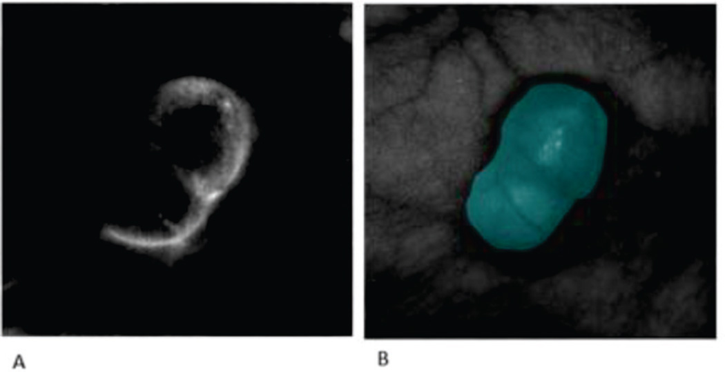
In order to evaluate the hyperspectral imaging and the classification method, a separate fluorescence image acquisition experiment was performed on the same mice. As the cancer cells had GFP signals, the fluorescence images were used to validate the cancer detection by the HSI classification method. After the HSI image acquisition, blue excitation at 455 nm and auto exposure time were selected for the fluorescence image acquisition. The GFP signals on the fluorescence images were manually segmented as the tumor region for validation in this HSI study. After image acquisition, tumors were resected horizontally for histological evaluation, which serves as the gold standard for cancer detection.

C. Overview of the Image Classification Method

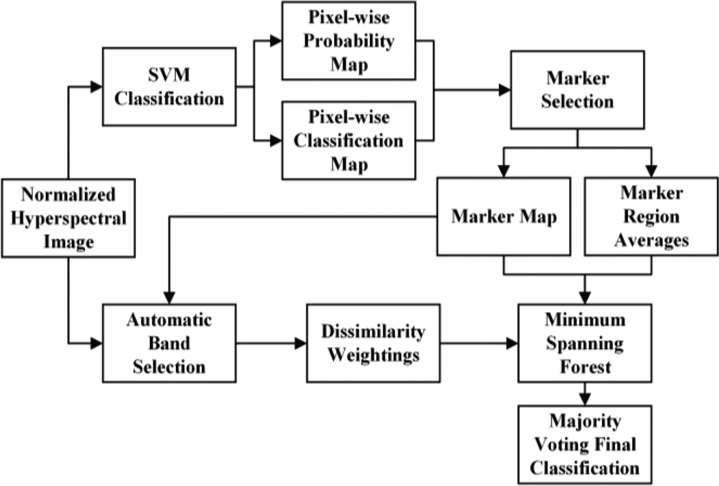
Fig. 1 shows a flow chart which summarizes the proposed classification method. The classification approach consists of six primary steps: (1) The images are preprocessed and normalized to intensity values ranging from 0 to 1; (2) An SVM classifier is used to perform pixel-wise classification based upon intensity; (3) Highly probable pixels are selected from the SVM results and are used as roots for the MSF; (4) Specific bands are automatically selected to use for edge weighting construction in the MSF; (5) The MSF is grown using the constructed weights and markers; (6) Majority voting is performed with the MSF results and the SVM pixel-wise classification. Details of this proposed method as well as image acquisition and the quantitative validation methods are provided in the following sections.

Fig. 1.

Flow chart of the classification algorithm using an SVM and MSF

D. SVM-based Classification

The first step in the image classification process involves the pixel-wise classification of the hyperspectral images. The pixel-wise classification result provides a framework for the MSF to be grown on, as well as highly probable markers that can be used to obtain approximations of average spectral values. SVMs are well suited for hyperspectral image classification at the pixel-wise level because they are able to provide accurate classification using low training data and large testing data sets. SVM’s are capable of processing large amounts of data and many features in training. For these hyperspectral images, each band’s intensity was used as a training feature. The SVM provides not only a classification map but also the probability of that classification which is used in the marker selection process. The SVM we used in this experiment comes from the LIBSVM [42]. For this study the Gaussian radial basis function was used as the kernel function which maps the data into a Hilbert space of infinite dimensions.

E. Connected Component Labeling and Marker Selection

After the SVM provides both pixel-wise classification and probability map, these maps are then used to select roots for which the MSF can be grown and the average spectral values can be obtained. The markers also play a key role in determining which bands should be used for dissimilarity measures; so accurate marker selection is a crucial step in this algorithm. The technique for marker selection that is used in this method is a probability-based method developed by Tarabalka et al [32], which makes use of both spatial information and probability information from the SVM. This method uses probability data and ensures that both highly probable pixels and large regions are given at least one marker.

Markers are selected using both spatial and probability information. For the spatial information a connected component labeling must first be performed. In this experiment, a connected component labeling algorithm that uses a union-find data structure was implemented in our method. The eight nearest neighbors surrounding each pixel were used to find connected components. The connected component labeling is performed on the SVM classification map to find connected regions of the same label type. Each of these connected regions are then evaluated individually and separated into two categories, large and small, based upon the total number of pixels M in that region. Large regions are regions that have M or greater pixels; and small regions are regions that contain fewer than M pixels. These small regions are not required to have multiple pixels, so a single pixel could be considered a small region. The following rules determine how markers are selected based upon the type of region:

1. For Large Regions with M or greater pixels, the top N percent of pixels within that region are selected as markers.

2. For Small Regions ranging from one to M-1 pixels, only pixels with a probability greater than P will be selected as markers.

The motivation for this method of marker selection comes from the observed over-classification when simple threshholding of probabilities was used. The inclusion of a spatial component allows for more accurate marker selection. It also forces those regions of sufficient size must contain at least one marker, eliminating one major cause of under-classification. It is important to note that the markers selected need not be spatially adjacent and are given independent labels in our algorithm following their selection. Previous studies [32] have associated all markers of the same type with one single tree root, the proposed method allows each marker to have its own root and later be classified by majority voting. This approach provides finer classification of spanning trees.

F. Automatic Band Selection

HSI provides a tremendous amount of data that can be used for classification. One major challenge in hyperspectral image processing is the elimination of noise from these large data sets. The band selection method works to eliminate the unnecessary bands in order to increase both efficiency and accuracy. It makes use of mutual information between the individual bands and the SVM classification labels. The mutual information is calculated from the standard entropy between each intensity based image band distribution and corresponding reference image created from the markers. The reference distribution is constructed from the cancerous labeled markers and the healthy tissue markers. The top X bands with the highest mutual information are then selected to be used for the dissimilarity measure. The mutual information between two distributions is given by:

$$I(X,Y)={\sum }_{x,y}p(x,y)\text{ log}\frac{p(x,y)}{p(x)p(y)}$$ (1)

where p(x) and p(y) are the probability distributions of X and Y and p(x,y) is the join probability distribution.

G. MSF based Spectral-Spatial Classification

An MSF provides the spatial component of this classification algorithm, while using spectral dissimilarity between pixels to control its growth. Given a set of well-selected markers an MSF is a powerful tool to accurately determine regional boundaries and is well suited for hyperspectral images. To grow an MSF, edge weightings between a pixel and its eight nearest neighbors were calculated with multiple dissimilarity measures in order to evaluate the most accurate measure. These measures include L1 vector norm, spectral angle mapper, spectral information divergence, normalized Euclidean distance, a combination of spectral angle mapper and spectral information divergence, spectral correlation measure, and a combination of derivative sign difference and spectral correlation measure.

Given two vector pixels p_i = (p_i1,…,p_iB) and p_j = (p_j1,…,p_jB) where B is the number of bands for each pixel, the L1 vector norm was calculated by the following equation:

$$\mathrm{L}1(p_i,p_j)={\sum }_{b=1}^B|p_{ib}-p_{jb}|$$ (2)

The spectral angle mapper (SAM) which incorporates differences in spectral shape is calculated by:

$$\mathrm{S}\mathrm{A}\mathrm{M}(p_i,p_j)={\mathbf{\text{cos}}}^{-\mathbf{1}}\frac{{\sum }_{\mathit{b}=\mathbf{1}}^{\mathit{B}}{\mathit{p}}_{\mathit{i}\mathit{b}}{\mathit{p}}_{\mathit{j}\mathit{b}}}{\sqrt{{\sum }_{\mathit{b}=\mathbf{1}}^{\mathit{B}}{{\mathit{p}}_{\mathit{i}\mathit{b}}}^{\mathbf{2}}{\sum }_{\mathit{b}=\mathbf{1}}^{\mathit{B}}{{\mathit{p}}_{\mathit{j}\mathit{b}}}^{\mathbf{2}}}}$$ (3)

The spectral information divergence (SID) [43] which also uses spectral shape and intensity is calculated by:

$$\mathrm{S}\mathrm{I}\mathrm{D}(p_i,p_j)=\mathrm{D}(p_i\Vert p_j)+\mathrm{D}(p_j\Vert p_i)$$ (4)

where,

$$\mathrm{D}(p_i\Vert p_j)=\sum _{\mathrm{k}=1}^{\mathrm{B}}{x}_k\text{ log }{x}_k/y_k$$

$$\mathrm{D}(p_j\Vert p_i)=\sum _{\mathrm{k}=1}^{\mathrm{B}}{y}_k\text{ log }{y}_k/x_k$$

The $x_k=\frac{p_{ik}}{{\sum }_{\mathrm{k}=1}^{\mathrm{B}}{p}_{ik}},y_{\mathrm{k}}=\frac{{\mathrm{p}}_{\mathrm{j}\mathrm{k}}}{{\sum }_{\mathrm{k}=1}^{\mathrm{B}}{\mathrm{p}}_{\mathrm{j}\mathrm{k}}}$ are probability distributions for pixel vector p_i, p_j, respectively.

The normalized Euclidean distance (NED) which is a normalized alternative to the L1 vector norm is given by:

$$\mathrm{N}\mathrm{E}\mathrm{D}(p_i,p_j)=\sqrt{{\sum }_{b=1}^B{(\frac{p_{ib}}{1/B{\sum }_{b=1}^B{p}_{ib}}-\frac{p_{jb}}{1/B{\sum }_{b=1}^B{p}_{jb}})}^2}$$ (5)

The product combination of spectral angle mapper and spectral information divergence (SIMSID) has been previously explored and is calculated as following:

$$\mathrm{S}\mathrm{A}\mathrm{M}\mathrm{S}\mathrm{I}\mathrm{D}(p_i,p_j)=\mathrm{S}\mathrm{A}\mathrm{M}(p_i,p_j)*\mathrm{S}\mathrm{I}\mathrm{D}(p_i,p_j)$$ (6)

The spectral correlation measure (SCM) which gives a normalized measure of spectral dissimilarity between 0 and 1 is given by:

$$\mathrm{S}\mathrm{C}\mathrm{M}(p_i,p_j)={\sum }_{b=1}^B|p_{ib}-p_{jb}|$$ (7)

The derivative sign difference (DSD) calculates the number of times the pixels’ spectral derivatives are of opposite signs and is calculated with the following method:

1. Calculate the first and second derivatives of the two pixel spectra’s to be considered.

2. Set the sign difference counter C to 0.

3. For each value of the derivatives if the sign of the first derivatives or the sign of the second derivatives are opposite increase C by 1.

4. Divide C by the total number of spectral bands.

The division by the total number of spectral bands ensures that the values of this measure fall between 0 and 1 and thus can be combined with the spectral correlation measure as defined by:

$$\mathrm{D}\mathrm{S}\mathrm{D}\mathrm{S}\mathrm{C}\mathrm{M}(p_i,p_j)=\mathrm{D}\mathrm{S}\mathrm{D}(p_i,p_j)*\mathrm{S}\mathrm{C}\mathrm{M}(p_i,p_j)$$ (8)

The spectral similarity scale (SSS) which combines a modified SCM with the Euclidean distance measure is given by:

$$\mathrm{S}\mathrm{S}\mathrm{S}(p_i,p_j)=\sqrt{1/B{\sum }_{b=1}^B[{(p_{ib}-p_{jb})}^2-{(1-r)}^2]}$$ (9)

Where r is given by:

$$\mathrm{r}=\frac{{\sum }_{b=1}^B[(p_{ib}-1/B{\sum }_{b=1}^B{p}_{ib})*(p_{jb}-1/B{\sum }_{b=1}^B{p}_{jb})]}{\sqrt{{\sum }_{b=1}^B{(p_{ib}-1/B{\sum }_{b=1}^B{p}_{ib})}^2*{\sum }_{b=1}^B{(p_{jb}-1/B{\sum }_{b=1}^B{p}_{jb})}^2}}$$ (10)

Once the edge weightings between all pixels have been calculated, to construct an MSF we first define the undirected graph G. This graph is constructed from the normalized hyperspectral image, where each pixel in a single plane is considered a vertex V, with edges E connecting a pixel to its surrounding neighbors. The set of weightings W calculated in numerous ways described above are used to quantify the edges E of this undirected graph. The graph G is then defined as G = (V, E, W), from which the spanning tree T can be grown.

From the undirected connected graph G a spanning tree T = (V, E_T) can be constructed while E_T is a subset of E. A minimum spanning tree, T_min, of the graph G is defined as the spanning tree T_min = (V, E _Tmin) such that the associated edge weightings W of T_min is minimal given as following:

$$T_{\mathit{\text{min}}}\in {\text{arg min}}_{T\in ST}\left\{{\sum }_{e_{i,j}\in E_T}{W}_{i,j}\right\}$$ (11)

Where ST is the set of all possible spanning trees constructed from the graph G [44].

Similarly a spanning forest F = (V, E_F) is defined as a non-connected graph without cycles while E_F is a subset of E, and the MSF F_min can be defined as following:

$$F_{\mathit{\text{min}}}\in {\text{arg min}}_{F\in SF}\left\{{\sum }_{e_{i,j}\in E_F}{W}_{i,j}\right\}$$ (12)

with SF being the set of all possible spanning forests, grown from the same roots, of the graph G. To grow an MSF on a specific set of M roots, additional vertices r_i, i = 1,‥…,M are added. These vertices connect the root r_i to a previously determined marker, and are used as the basis for the MSF growth. If an additional root R is added such that R is connected with null weighting to the additional vertices r_i, a minimum spanning tree of the graph G from the selected markers can be obtained. An MSF is then created when the vertex R is removed. Alternative minimum spanning tree algorithms can be implemented [45, 46], but Prim’s algorithm offers an efficient implementation when using a binary heap to store the edge weightings [47]. This algorithm allows for the time complexity of O(|E| log|V|) [48].

When using Prim’s algorithm to grow the MSF, the root markers and their associated edges are first added to a binary heap, while the vertices associated with these markers are added to the classification map. Iteratively, the edge of minimal weighting that does not connect to a currently labeled pixel is removed from the binary heap and that vertex is added to the classification map and is given the label of its associated marker. The edges of this vertex, which are not connected to an already labeled vertex, are then added to the binary heap. This iteration is repeated until all pixels in the classification map have been labeled, producing a classification map using an MSF [49].

This study used a new method for calculating dissimilarity while the MSF is being grown. The weightings are initially calculated using equations listed above. Prim’s algorithm iteratively adds the reaming edge weightings of each pixel that has been labeled. When these edges are added to the binary heap the modified algorithm creates new edge weightings that reflect the classification of the labeled marker to which they are associated. Two methods can then be used to construct these new weightings, the first method calculates an additional weighting between the connecting pixel and the markers from which that label is to be classified, thus comparing the pixel to the average spectral values of its potential label. The second method creates a weighting between the connecting pixel and all the pixels connected to that pixels branch of the MSF, causing branches to terminate more appropriately across gradients. These methods create a more robust segmentation process that better distinguishes along noisy gradients.

H. Majority Voting

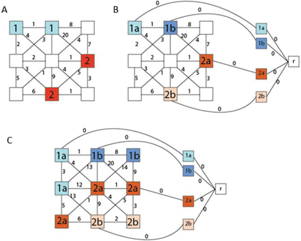
The initial classification of each pixel is determined from the label of the marker from which its spanning tree was formed. Since an MSF is an unconnected graph, it is ensured that there will only be one marker associated with each pixel. To account for potential errors in classification stemming from an initially misclassified marker, we introduce a majority-voting rule. Previous methods [50] have used connected components to determine regions and perform majority voting across entire regions. The method used here instead calls for a majority voting to be performed for each branch of the MSF. This is illustrated in Fig. 2. Each marker is given a unique label in the growing of the MSF allowing for a greater distinction across gradients when performing majority voting. This method allows not only for large regions to be reclassified, but also for region boundaries to be adjusted more finely, increasing accuracy along the SVM classification boundaries. This method calls first for a classification map to be constructed with each marker being given a unique label. Each branch of the MSF is evaluated separately by grouping together all pixels grown from their respective root, the mode of the SVM classification associated with these pixels gives the label to be assigned to the entire branch.

Fig. 2.

Flow Visualization of the MSF construction from the marker selection (A) to the marker labeling (B) and to the complete construction of the MSF (C) that will be classified with majority voting.

I. Classification Evaluation

To evaluate the accuracy of the automatic classification, four different measures were used as evaluation metrics: the overall accuracy (OA), sensitivity, and specificity [51, 52]. The overall accuracy is given by the number of pixels correctly classified divided by the total number of pixels in the image.

III. Results

A. Results of SVM and MI Band Selection

SVM is used to determine the most probable pixels to be selected and used as markers for the MSF. These results are also used in selecting the optimal bands for dissimilarity measures using mutual information. The SVM was able to accurately classify the image on a pixel-wise basis that was acceptable for automatic marker selection. By forcing a probability and region size threshold on the SVM classification, accurate markers were able to be determined and the appropriate bands were selected. These band ranges differed by images but agreed with previously tested band ranges using the GFP ground truth map. The most common band range with the highest mutual information was 800–870nm.

B. Evaluation of Simulation Images

Simulation images were first created to test the feasibility of this algorithm. The simulation images were created using randomly selected pixels from each mouse image. Seven generated simulation images consisted of a large cancerous region surrounded by smaller elliptical regions that also consist of cancerous pixels. The large cancerous region is made of randomly selected cancerous pixels well inside the tumor margin given by the ground truth map. The smaller regions are created by taking cancerous pixels on the boundary of healthy and cancerous tissue as given by the ground truth map. The rest of the simulation image pixels were given by randomly selected pixels from healthy normal tissue in each of the mouse images.

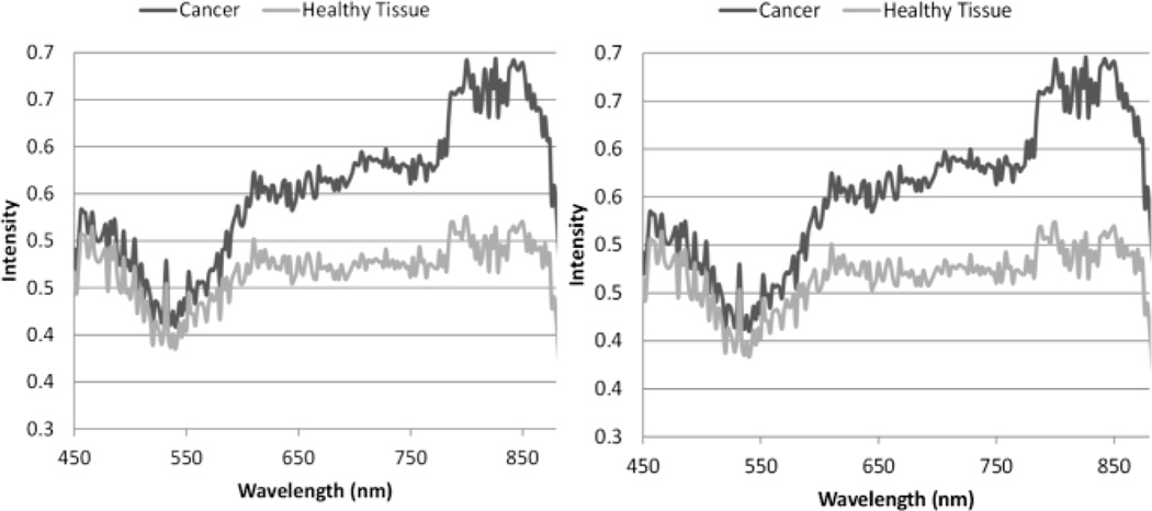
Fig. 3 demonstrates the average spectral values for the cancerous tissue and the healthy tissue of the simulation images and the in vivo mouse images, which are extremely similar between these two images. Fig. 4 shows the results of the SVM and the MSF on a simulation image as compared to the ground truth map. It is seen that the noisy simulation image is not well classified by the SVM based method; however reliable markers are able to be detected. The markers provide the initialization for the MSF to complete the classification with much higher accuracy. These results gave promise to the use of this algorithm on the real full in vivo images.

Fig. 3.

Average spectral values for pixels contained within the cancer and normal regions for the simulation (Left) and for in vivo mouse images (Right).

Fig. 4.

Classification results of the simulation image (A) compared to the gold standard (B), the SVM results (C) and the MSF method (D).

C. Edge Weighting Evaluations

The edge weightings dictate the MSF growth and therefore are crucial to accurate image classification. In this study, edges were separated into two types, i.e. edges that connect pixels of the same label, and edges that connect pixels of different labels, which were determined by the ground truth map. Histograms of these edge weightings were then constructed and evaluated to determine the effectiveness of the dissimilarity measure. The edge weightings were evaluated over three band ranges, the entire measured spectrum, a select grouping of bands determined by the automatic band selection, and the single optimal band. The spectral angle mapper dissimilarity measure produced the best results and was used to construct the histograms.

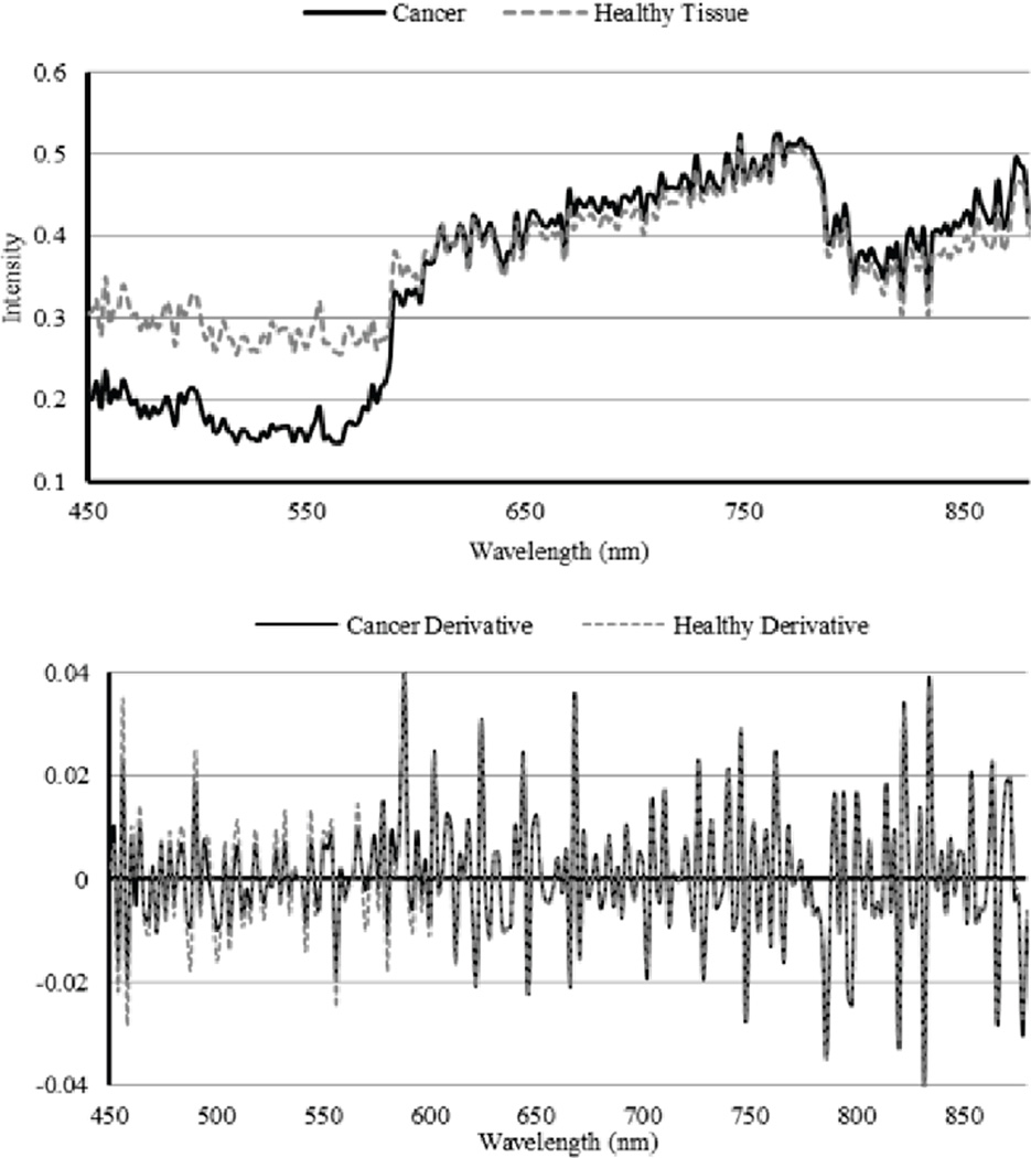
Dissimilarity measures are highly dependent upon both the spectral intensity and spectral shape of different tissue types. Fig. 5 shows an example of the average spectra of the cancerous tissue and the healthy tissue in a mouse image. The derivative of the spectra is also shown, and demonstrates how similar the spectral shape is between tissue types.

Fig. 5.

Spectral curves of the mouse image and the derivative of the image for both cancerous and healthy tissue.

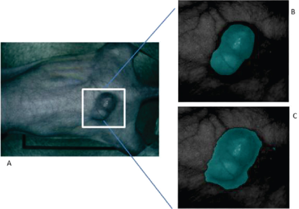
Fig. 6 shows an example classification of the mouse image using the spectral angle mapper dissimilarity measure which was found to be most effective. The GFP gold standard is shown in comparison of the MSF results. The segmentation result includes the shaded region surrounding the tumor which was not manually classified as cancerous when using the GFP standard.

Fig. 6.

RGB image of original mouse (A) and the corresponding gold standard image (B) with the classification result (C).

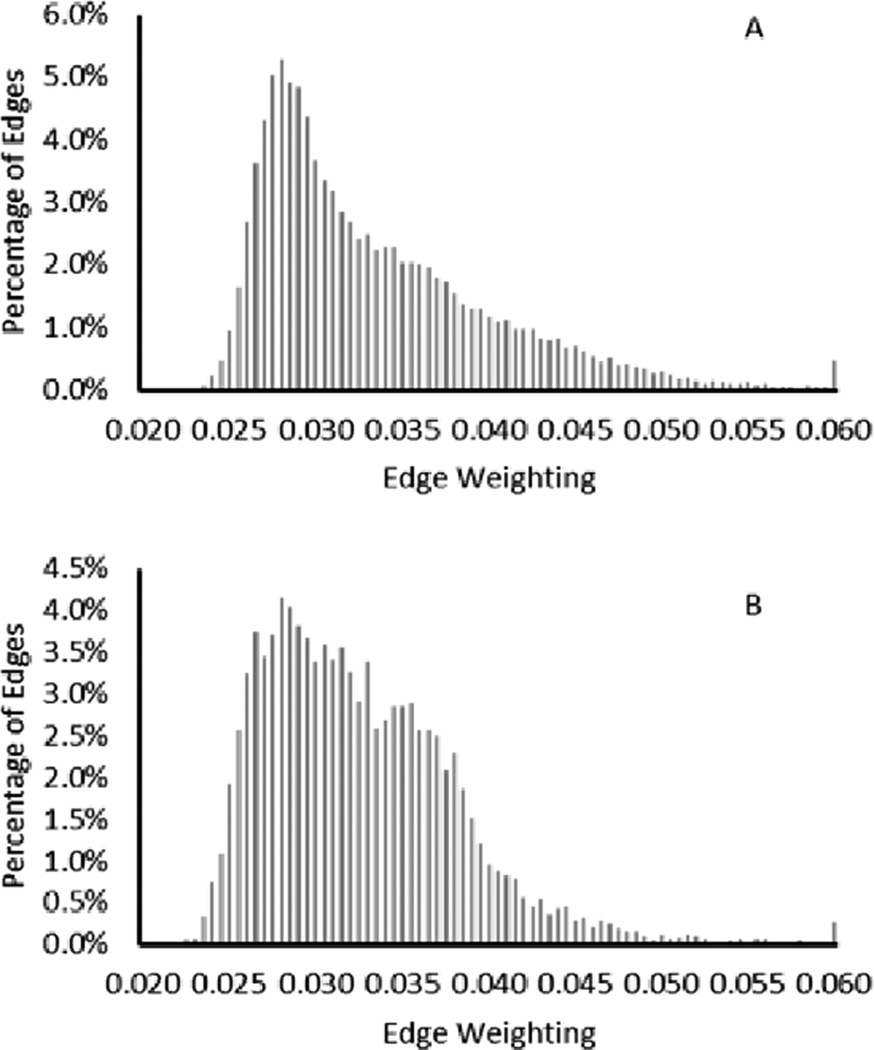
Fig. 7 shows the histogram of the edge weightings using all image bands. It is seen that the mean value of the edge weightings is slightly increased when the edges are connecting pixels of different labels. The mode of the edges connecting pixels of different type does not significantly differ from the mode of the edges connecting pixels of the same type.

Fig. 7.

Histogram of edge weightings for edges connecting pixels of the same label (A) and edges connecting pixels of different labels (B) using all image bands.

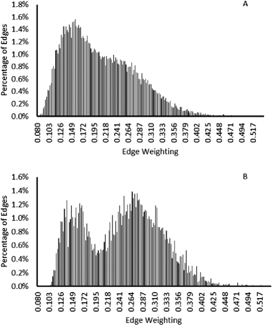
Fig. 8 shows the histogram of the edge weightings when the automatically selected bands were used to calculate the dissimilarity values. The mean value of the edge weightings shifts significantly for the edges connecting pixels of different type when compared to the edges connecting pixels of the same type. The mode of these edge weightings is also significantly different and increases for edges connecting pixels of different types. These results show the promising value in automatic band detection to eliminate unnecessary and inaccurate noise present in some image bands.

Fig. 8.

Histogram of edge weightings for edges connecting pixels of the same label (A) and edges connecting pixels of different labels (B) using select image bands.

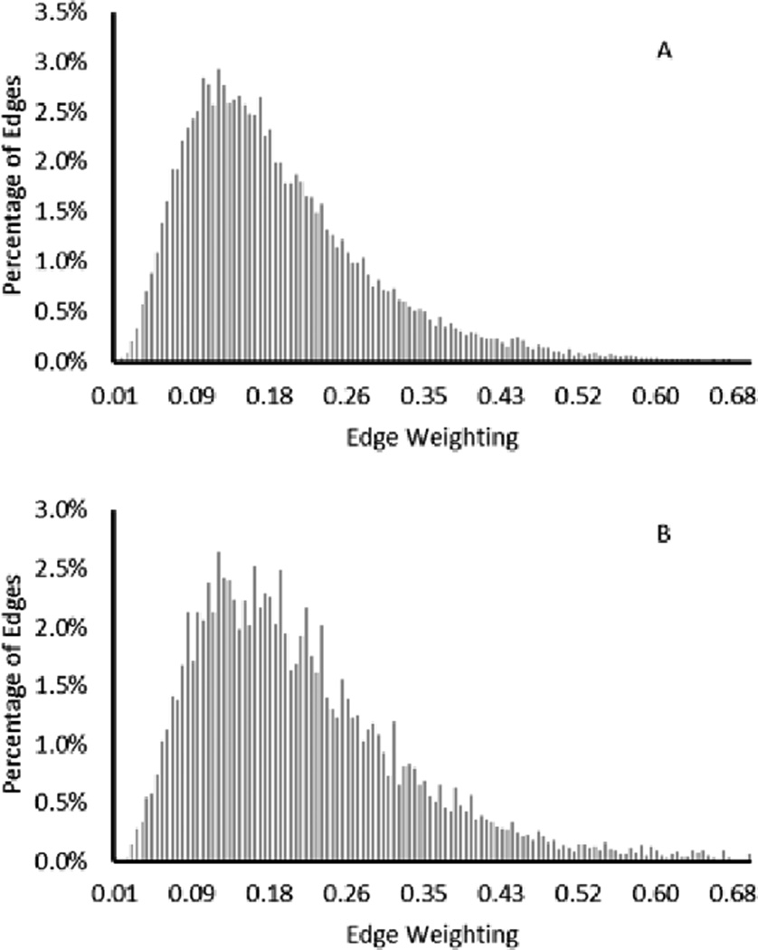
To test the results of the single optimal band, the histogram of edge weightings was calculated using only this band. Fig. 9 shows these histograms and demonstrates that the mean and mode were unchanged for pixels connecting the same and different tissue types. This result demonstrated the need for a wider range of bands to be used instead of a specific wavelength to detect cancerous tissue.

Fig. 9.

Histogram of edge weightings for edges connecting pixels of the same label (A) and edges connecting pixels of different labels (B) using a single image band.

Fig. 10 shows a graphical representation of the edge weightings and demonstrates the higher edge weightings present where tissue of different types meets. The edge weightings were calculated using a select band of wavelengths and using the spectral angle mapper function. The weightings show a strong dissimilarity surrounding the cancerous tissue which correlates to the high accuracy achieved by this segmentation.

Fig. 10.

Graphical representation of the edge weightings calculated with selected bands using the spectral angle mapper function (A) with the ground truth map (B) showing the border of the cancerous tissue.

D. Results of Minimum Spanning Forest with All Bands Used

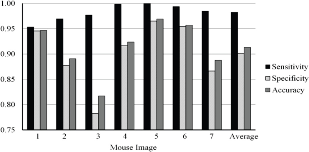
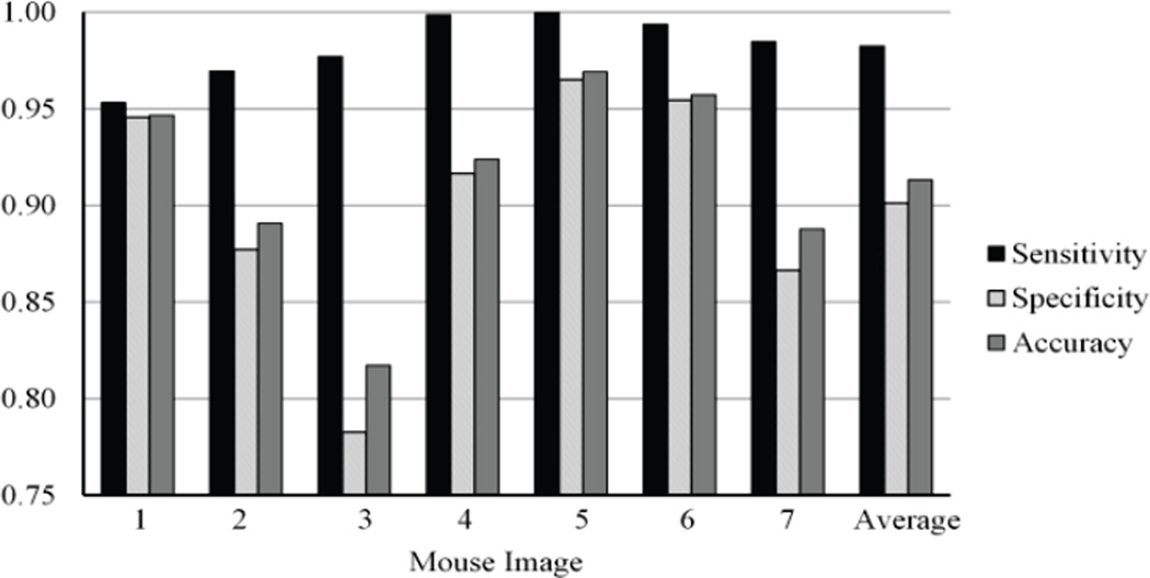
When edge weightings were calculated from all available bands of the hyperspectral image, the MSF based classification method was able to accurately classify the images with an average sensitivity of 98.2%, an average specificity of 90.4%, and an average overall accuracy of 91.6%. The normalized Euclidean distance measure and spectral angle mapper were most effective for the calculation of dissimilarity weightings. Fig. 11 shows the sensitivity, specificity, and overall accuracy for the MSF when the spectral angle mapper function was used to calculate dissimilarity. Table I shows the sensitivity, specificity, and accuracy results of all dissimilarity measures in all mouse images. This table shows that the normalized Euclidean distance measure and the spectral angle mapper function are the most accurate classification measures. The sensitivity of these results is consistently high at 98.2%.

Fig. 11.

The sensitivity, specificity, and overall accuracy of the MSF based classification method for cancer detection when the SAM dissimilarity measure and all image bands are used for the classification.

TABLE I.

The sensitivity, specificity, and overall accuracy for all dissimilarity measures over all images using all image bands

	Dis. Meas.	Image1	Image2	Image3	Image4	Image5	Image6	Image7
Sen	D1	0.988	0.743	0.795	0.981	1.000	0.479	0.809
	DSD	0.814	0.929	0.984	0.973	1.000	0.763	0.947
	L1	0.869	0.722	0.848	0.975	0.974	0.574	0.606
	L1p	0.793	0.756	0.880	0.987	0.987	0.609	0.631
	NED	0.949	0.969	0.977	0.997	1.000	0.995	0.986
	SAM	0.953	0.969	0.977	0.999	1.000	0.994	0.985
	SAM2	0.344	0.993	0.984	1.000	1.000	0.997	1.000
	SCM	0.983	0.965	0.977	1.000	1.000	0.984	0.983
	SID	0.987	0.961	0.977	1.000	1.000	0.996	0.993
	SIDSAM1	0.986	0.970	0.978	1.000	1.000	0.993	0.999
	SIDSAM2	0.986	0.969	0.979	1.000	1.000	0.992	1.000
	SSS	0.114	0.277	0.283	0.128	1.000	0.211	1.000
	D1	0.911	0.929	0.799	0.936	0.915	0.999	0.881
	DSD	0.960	0.681	0.487	0.974	0.761	0.979	0.874
Spe	L1	0.931	0.816	0.576	0.588	0.549	0.905	0.883
	L1p	0.939	0.797	0.550	0.585	0.519	0.810	0.789
	NED	0.947	0.878	0.782	0.939	0.964	0.954	0.865
	SAM	0.946	0.877	0.783	0.916	0.965	0.955	0.866
	SAM2	0.987	0.380	0.390	0.395	0.396	0.398	0.679
	SCM	0.909	0.874	0.782	0.820	0.968	0.956	0.836
	SID	0.729	0.729	0.483	0.472	0.741	0.766	0.602
	SIDSAM1	0.761	0.671	0.495	0.498	0.797	0.784	0.601
	SIDSAM2	0.839	0.722	0.535	0.529	0.835	0.802	0.651
	SSS	0.995	1.000	1.000	1.000	0.375	1.000	0.383
	D1	0.921	0.902	0.798	0.9405	0.925	0.964	0.869
	DSD	0.941	0.718	0.576	0.974	0.789	0.965	0.887
	L1	0.922	0.802	0.624	0.623	0.599	0.883	0.833
	L1p	0.919	0.791	0.609	0.6213	0.574	0.796	0.761
Acc	NED	0.948	0.891	0.817	0.944	0.969	0.957	0.886
	SAM	0.947	0.891	0.817	0.924	0.969	0.957	0.888
	SAM2	0.900	0.470	0.496	0.449	0.466	0.439	0.737
	SCM	0.919	0.887	0.817	0.836	0.971	0.958	0.862
	SID	0.764	0.763	0.571	0.520	0.771	0.781	0.672
	SIDSAM1	0.791	0.716	0.581	0.543	0.820	0.798	0.673
	SIDSAM2	0.858	0.758	0.614	0.572	0.854	0.814	0.714
	SSS	0.876	0.894	0.872	0.922	0.448	0.947	0.495

Dis. Meas. = Dissimilarity Measure, Sen = Sensitivity, Spe = Specificity, Acc = Accuracy

E. Minimum Spanning Forest with Selected Bands

The MSF was also constructed using an automatic band selection method that is implemented to reduce noise in unnecessary image bands. The bands that were automatically selected varied between images but mainly focused on the 800–870 nm range. Fig. 12 shows the sensitivity, specificity, and overall accuracy when the spectral angle mapper function was used to calculate dissimilarity over a specific band range. The band ranges were set at 60 nm to cover a broad region while being specific enough to eliminate noise. By using the select range of wavelengths the specificity and overall accuracy of the classification increased but the sensitivity decreased to an average sensitivity of 94.8%, an average specificity of 92.9%, and an average overall accuracy of 93.3%. These results shown an overall improvement as opposed to using all bands for classification and the improvements are shown in Table II. This table shows a comparison of the average results of the MSF when all bands or the selected bands are used to compute the edge weightings during the classification.

Fig. 12.

The sensitivity, specificity, and overall accuracy of the MSF based classification for cancer detection when the SAM dissimilarity measure and automatically selected bands are used for the classification.

TABLE II.

The average sensitivity, specificity, and overall accuracy for all dissimilarity measures

	All Bands
Dis. Meas.	Sensitivity	Specificity	Accuracy
D1	0.828 ± 0.19	0.910 ± 0.06	0.903 ± 0.06
DSD	0.916 ± 0.09	0.817 ± 0.18	0.835 ± 0.15
L1	0.795 ± 0.16	0.750 ± 0.17	0.755 ± 0.14
L1p	0.806 ± 0.15	0.713 ± 0.16	0.724 ± 0.13
NED	0.982 ± 0.02	0.904 ± 0.07	0.916 ± 0.05
SAM	0.982 ± 0.02	0.901 ± 0.06	0.913 ± 0.05
SAM2	0.902 ± 0.25	0.518 ± 0.23	0.565 ± 0.18
SCM	0.985 ± 0.01	0.878 ± 0.07	0.893 ± 0.06
SID	0.988 ± 0.01	0.646 ± 0.13	0.692 ± 0.11
SIDSAM1	0.989 ± 0.01	0.658 ± 0.13	0.703 ± 0.11
SIDSAM2	0.989 ± 0.01	0.702 ± 0.13	0.741 ± 0.11
SSS	0.431 ± 0.39	0.822 ± 0.30	0.779 ± 0.21
	Selected Bands
Dis. Meas.	Sensitivity	Specificity	Accuracy
D1	0.872 ± 0.15	0.901 ± 0.09	0.902 ± 0.07
DSD	0.862 ± 0.13	0.901 ± 0.13	0.901 ± 0.10
L1	0.740 ± 0.16	0.825 ± 0.14	0.821 ± 0.12
L1p	0.728 ± 0.15	0.812 ± 0.17	0.808 ± 0.14
NED	0.823 ± 0.14	0.959 ± 0.04	0.945 ± 0.03
SAM	0.948 ± 0.03	0.929 ± 0.06	0.933 ± 0.05
SAM2	0.647 ± 0.42	0.755 ± 0.24	0.744 ± 0.17
SCM	0.857 ± 0.20	0.935 ± 0.07	0.931 ± 0.05
SID	0.863 ± 0.17	0.793 ± 0.22	0.800 ± 0.18
SIDSAM1	0.866 ± 0.15	0.820 ± 0.19	0.825 ± 0.15
SIDSAM2	0.861 ± 0.15	0.852 ± 0.15	0.853 ± 0.12
SSS	0.523 ± 0.31	0.907 ± 0.11	0.869 ± 0.08

IV. Discussion

The proposed MSF based classification method has been shown to improve accuracy of the SVMs for detecting cancerous tissue. The tumors on the HSI images varied greatly in shape and size and were imaged through the skin of the host mice. The MSF when rooted on accurately selected seeds was able to expand within the region of the tumor to provide an accurate classification of the image. The improved marker selection tailored to cancerous tissue detection was able to supply accurate roots for the MSF. The markers were also used to eliminate unnecessary spectral bands that lead to improved dissimilarity measures. The modified majority voting presented in this method also proved to be a reliable method for correcting misclassified labels along regional boundaries, and thus improved the classification results along image gradients. The method is shown to accurately classify the tumor region with high sensitivity and accuracy.

The SVM classifier was able to accurately determine markers, which could be used to determine the most accurate range of bands for the dissimilarity measure to construct the edge weightings. The select bands proved to be able to eliminate the noise from the spectra and increased the accuracy of the classification methods. The errors found in these classification attempts were from large gradients and shaded regions of the images. Despite these errors the method was able to accurately classify the healthy and cancerous tissue in the hyperspectral images.

The use of automatic band selection has been shown to improve the accuracy of the image. It was observed that the MSF grew along the veins extending from the cancerous region. By using the select bands that do not contain the peak wavelengths observed from hemoglobin the specificity result was improved. The bands selected automatically varied between mice, however, all but one mouse contained the highest mutual information in the range of 800–880 nm. This wavelength is at the high end of the imaging device. Future studies could be performed in wavelengths above this range in the near infrared and infrared region.

The small errors present in the classification results were found in the areas of large gradients and shadowed regions. The shadows in these images can be addressed with modifications to the imaging techniques. The spectral angle mapper is specifically designed to be effective with images that contain shadows and was the most effective measure in this study. The further elimination of these shadowed regions may increase the accuracy of the segmentation process.

Errors in classification were observed when tumors were present on elevated parts of the mouse. The SVM struggled distinguishing a classification between cancerous tissue and elevated healthy tissue in those regions. These errors were less present in higher wavelength regions which show additional promise for extending the wavelength range into the infrared region. The MSF when given accurate markers was able to determine margins with promising accuracy for these regions where the SVM struggled to classify. The classification algorithm was written and run in MATLAB on Dual Intel Xeon 3.40 GHz CPUs with 256 GB of RAM. The SVM classified images in approximately 30 minutes and the MSF took approximately 15 minutes per image for classification. The speed can be significantly improved when the algorithm is implemented in C++ language.

The automatically selected spectral range for the majority of images was the 800–890 nm wavelengths. Using this spectral range the segmentation algorithm was able to successfully identify cancerous tissue with an average sensitivity of 94.8%, average specificity of 92.9%, and an average overall accuracy of 93.3%. These results were collected over 7 mice, each imaged over the wavelength of 450nm–950nm with the range 500–900nm being useful.

Further studies into the use of a higher wavelength range could warrant better classification results as the majority of spectral bands that contained valuable information were observed in the 800–870 nm range. The use of selected bands eliminated false positives that were observed in regions of high hemoglobin concentration extending from the tumor. Additional studies determining more wavelengths that can serve to better discriminate the cancerous region could be conducted, but the high accuracy observed in this study demonstrates the clear potential that this spectral spatial classification offers for in vivo cancer detection.

V. Conclusion

An MSF based classification method was proposed and evaluated for distinguishing cancerous from healthy tissue on hyperspectral images. The algorithm presented demonstrates an accurate means of classification of hyperspectral images for cancerous tissue detection. This method incorporates an SVM to perform an initial classification of the images providing accurate markers from which an MSF can accurately classify the cancerous and healthy tissue. The spectral bands of the hyperspectral image present rich information that can be used to distinguish cancerous and healthy tissue. The use of mutual information to eliminate unnecessary bands that caused misclassification proved valuable and allowed for great accuracy of the MSF. Edge weightings when calculated with a spectral angle mapper proved most accurate, particularly with images that contained regions with shadows. The hyperspectral imaging combined with automatic classification technique can have great potential for noninvasive cancer detection and may provide a promising tool for cancer imaging research and clinical applications.

References

- 1.Ferlay J, et al. Estimates of worldwide burden of cancer in 2008: GLOBOCAN 2008. Int J Cancer. 2010 Dec 15;127(12):2893–2917. doi: 10.1002/ijc.25516. [DOI] [PubMed] [Google Scholar]
- 2.Bedard N, et al. Emerging roles for multimodal optical imaging in early cancer detection: a global challenge. Technol Cancer Res Treat. 2010 Apr;9(2):211–217. doi: 10.1177/153303461000900210. [DOI] [PMC free article] [PubMed] [Google Scholar]
- 3.Fischer C, et al. Multispectral and hyperspectral imaging technologies in conservation: current research and potential applications. Studies in Conservation. 2006;51(Supplement-2):3–16. [Google Scholar]
- 4.Sokolov K, et al. Optical spectroscopy for detection of neoplasia. Curr Opin Chem Biol. 2002;6(5):651–658. doi: 10.1016/s1367-5931(02)00381-2. [DOI] [PubMed] [Google Scholar]
- 5.Ferris DG, et al. Multimodal Hyperspectral Imaging for the Noninvasive Diagnosis of Cervical Neoplasia. Journal of Lower Genital Tract Disease. 2001;5(2):65–72. doi: 10.1046/j.1526-0976.2001.005002065.x. [DOI] [PubMed] [Google Scholar]
- 6.Panasyuk SV, et al. Medical hyperspectral imaging to facilitate residual tumor identification during surgery. Cancer Biology & Therapy. 2007 Mar;6(3):439–446. doi: 10.4161/cbt.6.3.4018. [DOI] [PubMed] [Google Scholar]
- 7.Qi X, et al. A comparative performance study characterizing breast tissue microarrays using standard RGB and multispectral imaging. :75570Z–75570Z-8. [Google Scholar]
- 8.Masood K, et al. Spatial Analysis for Colon Biopsy Classification from Hyperspectral Imagery. Annals of BMVA. 2008;2008(4):1–16. [Google Scholar]
- 9.Kiyotoki S, et al. New method for detection of gastric cancer by hyperspectral imaging: a pilot study. J Biomed Opt. 2013;18(2):026010–026010. doi: 10.1117/1.JBO.18.2.026010. [DOI] [PubMed] [Google Scholar]
- 10.Dicker DT, et al. Differentiation of normal skin and melanoma using high resolution hyperspectral imaging. Cancer Biology & Therapy. 2006;5(8):1033–1038. doi: 10.4161/cbt.5.8.3261. [DOI] [PubMed] [Google Scholar]
- 11.Angeletti C, et al. Detection of malignancy in cytology specimens using spectral–spatial analysis. Laboratory investigation. 2005;85(12):1555–1564. doi: 10.1038/labinvest.3700357. [DOI] [PubMed] [Google Scholar]
- 12.Akbari H, et al. Hyperspectral imaging and quantitative analysis for prostate cancer detection. Journal of biomedical optics. 2012 Jul;17(7):076005. doi: 10.1117/1.JBO.17.7.076005. [DOI] [PMC free article] [PubMed] [Google Scholar]
- 13.Martin ME, et al. Development of an Advanced Hyperspectral Imaging (HSI) system with application for cancer detection. Annals of Biomedical Engineering. 2006;34(6):1061–1068. doi: 10.1007/s10439-006-9121-9. [DOI] [PubMed] [Google Scholar]
- 14.Roblyer D, et al. Multispectral optical imaging device for in vivo detection of oral neoplasia. J Biomed Opt. 2008;13(2):024019–024019. doi: 10.1117/1.2904658. [DOI] [PMC free article] [PubMed] [Google Scholar]
- 15.Liu Z, et al. Tongue Tumor Detection in Medical Hyperspectral Images. Sensors. 2012;12(1):162–174. doi: 10.3390/s120100162. [DOI] [PMC free article] [PubMed] [Google Scholar]
- 16.Lu G, et al. Hyperspectral Imaging for Cancer Surgical Margin Delineation: Registration of Hyperspectral and Histological Images. Proc SPIE. 2014;9036:90360s. doi: 10.1117/12.2043805. [DOI] [PMC free article] [PubMed] [Google Scholar]
- 17.Lu G, et al. Estimation of tissue optical parameters with hyperspectral imaging and spectral unmixing. Proc SPIE. 2015;9417:94170Q. doi: 10.1117/12.2082299. [DOI] [PMC free article] [PubMed] [Google Scholar]
- 18.Lu G, et al. Quantitative wavelength analysis and image classification for intraoperative cancer diagnosis with hyperspectral imaging. Proc. SPIE. 2015;9415:94151B. doi: 10.1117/12.2082284. [DOI] [PMC free article] [PubMed] [Google Scholar]
- 19.Fei B, et al. WE-D-9A-05: Medical Hyperspectral Imaging for the Detection of Head and Neck Cancer in Animal Models. Medical Physics. 2014;41(6):500–501. [Google Scholar]
- 20.Isabelle M, et al. Correlation mapping: rapid method for identification of histological features and pathological classification in mid infrared spectroscopic images of lymph nodes. Journal of Biomedical Optics. 2010;15(2):026030–026030-5. doi: 10.1117/1.3386061. [DOI] [PubMed] [Google Scholar]
- 21.Gebhart SC, et al. Liquid-crystal tunable filter spectral imaging for brain tumor demarcation. Appl Opt. 2007 Apr 1;46(10):1896–1910. doi: 10.1364/ao.46.001896. [DOI] [PubMed] [Google Scholar]
- 22.Lu G, et al. Medical hyperspectral imaging: a review. Journal of Biomedical Optics. 2014;19(1):010901. doi: 10.1117/1.JBO.19.1.010901. [DOI] [PMC free article] [PubMed] [Google Scholar]
- 23.Akbari H, et al. Detection of Cancer Metastasis Using a Novel Macroscopic Hyperspectral Method. Proc SPIE. 2012;8317:831711. doi: 10.1117/12.912026. [DOI] [PMC free article] [PubMed] [Google Scholar]
- 24.Akbari H, et al. Hyperspectral imaging and quantitative analysis for prostate cancer detection. J Biomed Opt. 2012;17(7):076005. doi: 10.1117/1.JBO.17.7.076005. [DOI] [PMC free article] [PubMed] [Google Scholar]
- 25.Lu G, et al. Spectral-Spatial Classification Using Tensor Modeling for Cancer Detection with Hyperspectral Imaging. Proc SPIE. 2014;9034:903413. doi: 10.1117/12.2043796. [DOI] [PMC free article] [PubMed] [Google Scholar]
- 26.Lu G, et al. Spectral-spatial classification for noninvasive cancer detection using hyperspectral imaging. J Biomed Opt. 2014;19(10):106004. doi: 10.1117/1.JBO.19.10.106004. [DOI] [PMC free article] [PubMed] [Google Scholar]
- 27.Bernard K, et al. Spectral-Spatial Classification of Hyperspectral Data Based on a Stochastic Minimum Spanning Forest Approach. Image Processing, IEEE Transactions on. 2012;21(4):2008–2021. doi: 10.1109/TIP.2011.2175741. [DOI] [PubMed] [Google Scholar]
- 28.Pike R, et al. A Minimum Spanning Forest Based Hyperspectral Image Classification Method for Cancerous Tissue Detection. Proc SPIE. 2014;9034:90341w. doi: 10.1117/12.2043848. [DOI] [PMC free article] [PubMed] [Google Scholar]
- 29.Meyer F. Minimum Spanning Forests for Morphological Segmentation. In: Soille P, editor. Mathematical Morphology and Its Applications to Image Processing, Computational Imaging and Vision J. Serra. Netherlands: Springer; 1994. pp. 77–84. [Google Scholar]
- 30.Xu Y, et al. 2D image segmentation using minimum spanning trees. Image and Vision Computing. 1997;15(1):47–57. [Google Scholar]
- 31.Abdel-Mottaleb M, et al. Face detection in complex environments from color images. International Conference on Image Processing. 1999;3:622–626. 1999. [Google Scholar]
- 32.Tarabalka Y, et al. Segmentation and Classification of Hyperspectral Images Using Minimum Spanning Forest Grown From Automatically Selected Markers. Systems, Man, and Cybernetics, Part B. Cybernetics, IEEE Transactions on. 2010;40(5):1267–1279. doi: 10.1109/TSMCB.2009.2037132. [DOI] [PubMed] [Google Scholar]
- 33.Tarabalka Y, et al. Spectral-spatial classification of hyperspectral images using hierarchical optimization. Hyperspectral Image and Signal Processing: Evolution in Remote Sensing (WHISPERS), 2011 3rd Workshop on; 6–9 June 2011; 2011. pp. 1–4. [Google Scholar]
- 34.Bernard K, et al. Spectral-Spatial Classification of Hyperspectral Data Based on a Stochastic Minimum Spanning Forest Approach. Ieee Transactions on Image Processing. 2012 Apr;21(4):2008–2021. doi: 10.1109/TIP.2011.2175741. [DOI] [PubMed] [Google Scholar]
- 35.Champion A, et al. Semantic interpretation of robust imaging features for Fuhrman grading of renal carcinoma. Engineering in Medicine and Biology Society (EMBC), 2014 36th Annual International Conference of the IEEE; 26–30 Aug, 2014; pp. 6446–6449. [DOI] [PMC free article] [PubMed] [Google Scholar]
- 36.Chapelle O, et al. Support vector machines for histogram-based image classification. Neural Networks, IEEE Transactions on. 1999;10(5):1055–1064. doi: 10.1109/72.788646. [DOI] [PubMed] [Google Scholar]
- 37.Cheng-Hsuan L, et al. A Spatial-Contextual Support Vector Machine for Remotely Sensed Image Classification. Geoscience and Remote Sensing, IEEE Transactions on. 2012;50(3):784–799. [Google Scholar]
- 38.Z J, Li XR, Wang J, Zhao LY. Hyperspectral image classification based on compsite kernels support vector machine. Zhejiang Daxue Xuebao (Gongxue Ban)/Journal of Zhejiang University (Engineering Science) 2013;47(8):1403–1410. [Google Scholar]
- 39.Priego B, et al. Hyperspectral image segmentation through evolved cellular automata. Pattern Recognition Letters. 2013;34(14):1648–1658. [Google Scholar]
- 40.Fei B, et al. Hyperspectral imaging and spectral-spatial classification for cancer detection. Biomedical Engineering and Informatics (BMEI), 2012 5th International Conference on; 16–18 Oct. 2012; 2012. pp. 62–64. [Google Scholar]
- 41.Wang D, et al. The pivotal role of integrin β1 in metastasis of head and neck squamous cell carcinoma. Clinical Cancer Research. 2012;18(17):4589–4599. doi: 10.1158/1078-0432.CCR-11-3127. [DOI] [PMC free article] [PubMed] [Google Scholar]
- 42.Chang C-C, et al. LIBSVM: A library for support vector machines. ACM Transactions on Intelligent Systems and Technology (TIST) 2011;2(3):27. [Google Scholar]
- 43.Chein IC. An information-theoretic approach to spectral variability, similarity, and discrimination for hyperspectral image analysis. Information Theory, IEEE Transactions on. 2000;46(5):1927–1932. [Google Scholar]
- 44.Stawiaski J. Ph.D. dissertation. Paris, France: Paris School Mines; 2008. Mathematical morphology and graphs: Application to interactive medical image segmentation. [Google Scholar]
- 45.Gabow H, et al. Efficient algorithms for finding minimum spanning trees in undirected and directed graphs. Combinatorica. 1986;6(2):109–122. [Google Scholar]
- 46.Kruskal JB. On the shortest spanning subtree of a graph and the traveling salesman problem. Proceedings of the American Mathematical society. 1956;7(1):48–50. [Google Scholar]
- 47.Prim RC. Shortest Connection Networks And Some Generalizations. Bell System Technical Journal. 1957;36(6):1389–1401. [Google Scholar]
- 48.Moret BE, et al. An empirical analysis of algorithms for constructing a minimum spanning tree. In: Dehne F, Sack J-R, Santoro N, editors. Algorithms and Data Structures, Lecture Notes in Computer Science. Berlin Heidelberg: Springer; 1991. pp. 400–411. [Google Scholar]
- 49.Cormen TH, et al. Introduction to Algorithms, Third Edition. The MIT Press; 2009. [Google Scholar]
- 50.Tarabalka Y, et al. Segmentation and Classification of Hyperspectral Images Using Minimum Spanning Forest Grown From Automatically Selected Markers. Ieee Transactions on Systems Man and Cybernetics Part B-Cybernetics. 2010 Oct;40(5):1267–1279. doi: 10.1109/TSMCB.2009.2037132. [DOI] [PubMed] [Google Scholar]
- 51.Lu G, et al. Bleeding detection in wireless capsule endoscopy images based on color invariants and spatial pyramids using support vector machines; Engineering in Medicine and Biology Society, EMBC, 2011 Annual International Conference of the IEEE; 2011. pp. 6643–6646. [DOI] [PubMed] [Google Scholar]
- 52.Qin X, et al. Breast tissue classification in digital tomosynthesis images based on global gradient minimization and texture features. Proc. SPIE 9034. 2014;9034:90341V–90341V-8. doi: 10.1117/12.2043828. [DOI] [PMC free article] [PubMed] [Google Scholar]