

Abstract
We have developed a simple and efficient algorithm to identify each member of a large collection of DNA-linked objects through the use of hybridization, and have applied it to the manufacture of randomly assembled arrays of beads in wells. Once the algorithm has been used to determine the identity of each bead, the microarray can be used in a wide variety of applications, including single nucleotide polymorphism genotyping and gene expression profiling. The algorithm requires only a few labels and several sequential hybridizations to identify thousands of different DNA sequences with great accuracy. We have decoded tens of thousands of arrays, each with 1520 sequences represented at ∼30-fold redundancy by up to ∼50,000 beads, with a median error rate of <1 × 10⁻⁴ per bead. The approach makes use of error checking codes and provides, for the first time, a direct functional quality control of every element of each array that is manufactured. The algorithm can be applied to any spatially fixed collection of objects or molecules that are associated with specific DNA sequences.
Microarray technology, devised for the analysis of complex biological systems, uses the ability of a DNA strand to hybridize specifically to its complement to extract 1000s of measurements at a time from a single sample (Watson and Crick 1953; Southern et al. 1992; Pease et al. 1994; Schena et al. 1995; Chee et al. 1996; Lockhart et al. 1996; Lockhart and Winzeler 2000). Although relatively new, this technology has enabled a variety of important applications, for example, genome-wide quantitative analysis of gene expression and large-scale single nucleotide polymorphism (SNP) discovery and genotyping (Chee et al. 1996; Lockhart et al. 1996; Wang et al. 1998; Fan et al. 2003; Hardenbol et al. 2003; Kennedy et al. 2003; Yvert et al. 2003). Microarrays are also beginning to play a role in the reinvention of cancer classification and drug discovery (Johnson et al. 2002; van't Veer et al. 2002).
Conventional microarrays are manufactured by spotting or synthesizing probes at known locations on a two-dimensional substrate (Fodor et al. 1991; Schena et al. 1995; Holloway et al. 2002). The significance of our novel approach is that it enables the production of randomly assembled arrays in which the location of a probe is initially unknown (Michael et al. 1998). Random bead loading combined with decoding avoids the need for physical addressing of each element and thus achieves unprecedented levels of miniaturization and very high packing densities by using relatively simple bulk processes (Figs. 1, 2). For example, a typical spotted array with 100-μm center-to-center spacing has ∼400-fold lower packing density, and a photolithographically synthesized array (Fodor et al. 1991) with 11-μm center-to-center spacing has about fourfold lower density than that of the arrays described here. The random assembly of 300-nm-diameter beads in 500-nm wells has been reported, a density ∼40,000 times higher than that of a typical spotted microarray (Michael et al. 1998).
Figure 1.
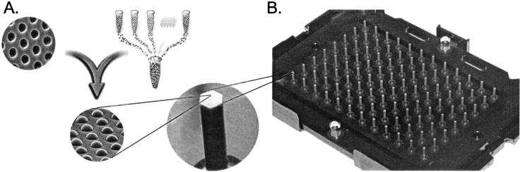
Assembly of a random array. (A) Creation of a bead pool and assembly into ∼3-μm-diameter wells etched in optical fiber bundles. Once a bead pool is made, it is relatively straightforward to assemble and decode large numbers of arrays. Each array contains ∼50,000 beads distributed among 1520 bead types, so that each bead type is represented at ∼30-fold redundancy. Scanning electron micrographs are shown of an unassembled and an assembled array containing one bead per well. (B) Because individual arrays are only ∼1.4 mm in diameter, they can easily be arranged into a 96-array matrix, designed for parallel analysis of samples in standard microtiter plates.
Figure 2.
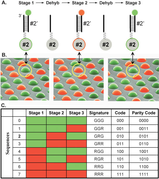
Decoding process. (A) The sequential hybridization process is illustrated for a single bead, of bead type 2. In stage 1, a complementary decoder hybridizes to the oligonucleotide probe that is attached to the bead (for details of the procedure, see Methods). The decoder is labeled with a fluorophore (green in stage 1, red in stage 2, and green in stage 3). The fluorescent signal is read by imaging the entire array. The array is then dehybridized, and the process is repeated for two more stages. (B) A scanning electron micrograph of an array of beads, artificially colored to represent three sequential hybridization stages. The images, taken collectively, reveal a combinatorial code for each bead. Note that the bead circled in yellow has the color signature GRG or code 010. (C) Colors, or states, are assigned to individual decoder sequences in each stage to produce a unique combination across stages. This signature, or code, identifies each bead type. As indicated in the parity code column, an extra decoding stage (data not shown) can be performed to provide an error checking parity bit. After three stages of decoding, all the beads are uniquely identified by their color.
Although randomly assembled arrays were recognized from the outset as a potentially revolutionary approach to microarray technology, the initial attempts to determine the location and identity of beads could only distinguish a few codes, limiting the usefulness of the approach (Michael et al. 1998). These initial attempts at decoding relied on dye impregnation of beads, but this approach suffered from variability in quantitation, lack of stability, and other problems. A number of other schemes that aim to encode particles directly with combinatorial codes generated by mixtures or spatial arrangements of optical signaling molecules have similar issues (Fulton et al. 1997; Han et al. 2001; Lockhart and Trulson 2001; Nicewarner-Pena et al. 2001; Braeckmans et al. 2002; Chan et al. 2002). We sidestepped the need for complex dye chemistries and painstaking labeling processes by devising a novel, highly efficient decoding algorithm that uses the specificity and reversibility of DNA hybridization.
RESULTS
Design of DNA-Based Decoding
Our algorithm uses sequential hybridizations of dye-labeled oligonucleotides, or decoders, complementary to bead sequences to create a combinatorial decoding scheme for arrays. It is distinct from sequencing by hybridization (SBH), which has been used successfully to characterize sequences de novo by hybridization to all n-mers or a well-chosen subset, typically in the range of 4- to 10-mers (Drmanac et al. 1996, 1998; Gunderson et al. 1998; Brenner et al. 2000). Our approach uses longer sequences, each designed to hybridize to a defined target with high specificity. It is capable of decoding, with high accuracy, many 1000s of bead types. Each bead type is defined by a unique DNA sequence that is recognized by a complementary decoder.
To illustrate, we show an example of decoding eight different bead types. We use two fluorescent labels, or states (green and red) in combination with three sequential hybridizations, or stages. The sequential hybridization process is illustrated for a single bead (bead type 2 of eight) in Figure 2A. In each of the three stages, the bead is “colored” by hybridization to a fluorescently labeled decoder oligonucleotide (Fig. 2A,B). In practice, all beads in the array are labeled simultaneously at each stage, by exposure to a pooled set of decoders, so that the process is intrinsically parallel and efficient.
The combinatorial assignment of green and red within each pool of eight decoders is shown in Figure 2C. There are three decoder pools in total, one for each stage. The stage 1 pool has the first four decoders colored green and the last four colored red. The decoders in subsequent stages are labeled so that after three stages each bead type is assigned a unique three-bit color code. Note that the sequences of the decoders are unchanged from stage to stage; only the fluorescent labels are varied. The bead circled in Figure 2B has the color signature (GRG), or 010 code in binary representation, in which G = 0 and R = 1. Its sequence can be identified as sequence 2 by referring to the color-lookup table in Figure 2C. Although assignment of codes to sequences is unambiguous after three stages, additional stages can be added for error checking purposes (last column of Fig. 2C) to be described below.
In this simple fashion, the eight bead types are decoded with three stages and two color labels. The approach scales exponentially. If there are N bead types and k distinguishable labels, or states, then the number of stages required is  . Thus, a large number of sequences can be decoded by using only a few labels across a few stages. For instance, four states (colors) combined with eight decoding stages enables up to 65,536 (48) different bead types to be decoded.
There are a number of ways of creating different states. Distinct fluorescent labels can be used as described in Figure 2, or the intensity levels of fluorescent labels can be varied to create grayscale states. We use a process that decodes 1520 different bead types by using three states: two fluorescent “ON” states (FAM and CY3 fluorescent labels) and one nonfluorescent “OFF” state. The logarithmic relationship between the number of bead types and the number of decode stages shows that the 1520 bead types can be decoded in only  stages. In practice, we use an additional stage to enable error checking. Without error checking, a single mistake in resolving a color label in any of the decode stages will lead to misclassification of a bead. This could result from, for example, a weak fluorescent signal or a speck of dust on the array.
Error Checking
The error-checking concepts that we have developed, and that underlie the robustness of our hybridization-based approach, are based on algorithms from digital information theory (Shannon 1948a,b; Hamming 1986). Although they are well known in other fields, they have not, to our knowledge, previously been applied to microarray manufacture or, indeed, more generally to DNA hybridization. With functional testing of every element of every array, we achieve a level of quality control that is unprecedented in microarray manufacture. As a result, we overcome some of the challenges in quality control that can plague the manufacture of ordered microarrays, which can also suffer from random sources of error (Hubbell and Pevzner 1999; Battaglia et al. 2000; Taylor et al. 2001; Sengupta and Tompa 2002; Shearstone et al. 2002; Hessner et al. 2003).
The simplest form of error checking we have used has a parity bit and is illustrated in Figure 2C. The assigned four-bit codes all have an even parity bit sum and are termed valid codes. An error in a single decode stage is a one-bit error that creates an odd parity, or invalid code. Although the parity-based approach is effective, we have optimized error checking by designing a more advanced scheme that assigns codes in a way that takes into account inherent biases in error rates and enables estimation of the misclassification rate.
In our implementation of three-state decoding, the most common errors are transitions from an ON state, one or two, to the OFF state, zero. Less common are transitions from OFF to ON. Transitions from one ON state to the other ON state are extremely rare. This can be explained by the fact that such transitions require two simultaneous classification errors: a mistaken ON in one color channel and a mistaken OFF call in the other color channel. We used these biases in error rates by designing the decode stages so that every valid code has a fixed number of OFF states. For example, if there are 1520 bead types and we use three-state eight-stage decoding, then each valid code would be designed to be OFF in exactly two stages and ON in exactly six stages (the actual scheme used is a slight variant on this design; see Methods). An example of a valid code would be 21110210.
With this scheme, it is theoretically impossible to misclassify a code through any number of occurrences of the most common error type: a transition from an ON state to an OFF state. The following events can lead to misclassification: a transition from one ON state to the other, or multiple stage errors with at least one ON-to-OFF transition and at least one OFF-to-ON transition. Both events are extremely rare. The space of all possible color codes is divided into three categories: used valid, unused valid, and invalid (Table 1). The unused valid codes represent codes that could be assigned to bead types but are not currently in use. Monitoring the number of beads decoding to this category allows an estimation of the true misclassification rate, as described in the Methods section. With little extra cost to the overall process, this error checking scheme monitors the rate of single state errors, minimizes the number of misclassified beads, and permits the number of misclassified beads, one of the key determinants of array quality, to be estimated.
Table 1.
Distribution and Use of 6561 Codes in the Three-State, Eight-Stage System
| Type | Number | Purpose |
|---|---|---|
| Used valid codes | 1520 | Assigned to actual beads. |
| Unused valid codes | 272 | Detect rare two-stage errors. |
| Estimate the number of misclassification events. | ||
| Invalid codes | 4769 | Detect single stage errors. |
| Monitor overall decode process; useful for detecting occasional catastrophic failures. |
Decoding of Randomly Assembled Arrays
By using this approach, arrays of 1520 different bead types (∼50,000 total beads) were decoded 96 at a time in the Sentrix array matrix format. Representative examples from the decoding are shown in Figure 3, and summary statistics are presented in Table 2. Figure 3A shows a set of hybridization images from all eight stages of the decoding process. High signal to noise allows the code of the circled bead to be read by eye. The code is 11012202, with FAM = 1, Cy3 = 2, and OFF = 0. Furthermore, we can identify this as a valid used code according to the error checking scheme. Figure 3B shows an example of decoding data for a population of beads from a single array imaged in the FAM channel for one out of the eight decode stages. The clear separation between the two modes in the histogram indicates that most beads can be classified unambiguously as OFF or ON. Information of this type is the input for histogram-based or stage-by-stage decoding, which is used for quality control of individual stages. Actual decoding is carried out by using a core-by-core classification algorithm, which makes use of the fluorescence intensity profile of each bead, measured in FAM and Cy3 channels, across all eight decode stages (Fig. 3C) to classify a bead as ON or OFF. In the example of Figure 3C, the code is 02212110.
Figure 3.
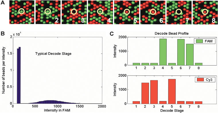
(A) Decoding images from eight sequential stages (numbered). Each image is a false-color composite of the FAM and Cy3 grayscale images from each stage. A small region (<0.2%) of a single array is shown. The circled bead is one of up to ∼4.8 million in a single 96-array matrix. It has the code 11012202. A total of 1728 images, each ∼5 Mb in size and containing ∼1.7 million pixels, are collected in order to decode an array matrix. (B) Histogram of bead intensities for a single stage. The low intensity peak includes beads in the OFF state and empty wells. The higher intensity peak includes beads in the ON state. (C) The eight-stage intensity profile of a typical individual bead (code = 02212110) in the FAM and Cy3 channels (∼100 counts of intensity are from camera DC offset).
Table 2A.
Quality Measures for a Random Sampling of 100 Recently Manufactured Array Matrices, Comprising a Total of 9600 Arrays.
| Average beads in used | Average beads in unused | Average beads in invalid | |
|---|---|---|---|
| All arrays | 46,576 | 0.14 | 153 |
| Array matrix 1 | 48,653 | 0.21 | 202 |
| Array matrix 2 | 46,872 | 0.29 | 106 |
| Array matrix 3 | 48,500 | 0.04 | 70 |
| Array matrix 4 | 45,367 | 0.09 | 90 |
| Array matrix 5 | 44,898 | 0.85 | 252 |
| Array matrix 6 | 46,549 | 0.77 | 172 |
| Array matrix 7 | 46,480 | 0.20 | 106 |
| Array matrix 8 | 46,596 | 0.17 | 88 |
| Array matrix 9 | 46,837 | 0.06 | 84 |
| Array matrix 10 | 48,260 | 0.04 | 89 |
The first row of the table provides averages over all arrays, and other rows provide data on a subset of 10 randomly chosen array matrices. The results shown are based on raw data, prior to the application of any quality control filters.
Table 2B.
Summary Statistics for the 9600 Arrays
| Worst percentile | Mean | Best percentile | |
|---|---|---|---|
| Bead types decoded | 1520 | 1520 | 1520 |
| Decode efficiency | 97.6% | 99.6% | 99.9% |
| Misclassification rate | 1.4 × 10⁻⁴ | 1.2 × 10⁻⁵ | 0 |
Decode efficiency is the number of valid signatures assigned, divided by the total number of beads in the array.
By using the core-by-core algorithm, we have decoded many 10s of 1000s of arrays with a median random error rate of <1 × 10⁻⁴ per bead (Table 2). The rate was estimated by using the error checking scheme summarized in Table 1. To get a more direct measure of random error rates, we decoded a matrix of 96 arrays twice and considered beads that were decoded to used codes in both decoding events (average of 44,912 ± 1098 beads/array). The misclassification rate was then estimated by dividing the number of discrepant calls by the total number of calls. This is an upper bound on the rate, as the errors are distributed among the two decoding events. The mean misclassification rate obtained in this way was 3.8 × 10⁻⁵ with a 95% confidence interval of zero to 1.8 × 10⁻⁴. The results are consistent with the estimates obtained in Table 2. This analysis does not account for any systematic misclassification errors, but functional tests (e.g., genotyping comparison studies with other technologies) have not identified any systematic misclassification (data not shown).
Error Rate Impact
The error rate of <1 × 10⁻⁴ per bead has a negligible impact on assay accuracy because of the ∼30-fold average redundancy and fivefold minimum redundancy of each bead type (Fig. 4). The measured decoding error rate translates to a median of fewer than five misclassified beads per array. Therefore, the chances of more than one random error affecting a given bead type are very low (∼5 × 10⁻⁶). Given the fact that outlier removal is used in our downstream processes, we estimate that a 100-fold higher average random error rate would have to occur in order to affect our assays (the calculation assumes that the assay is affected if any one bead type on the array has >10% of beads mis-decoded). If we did not use an extra stage for error checking and the number of possible codes was equal to the number of used codes, then any single stage error would lead to misclassification of a bead. Based on the average number of invalid codes generated by our process, we estimate that the average misclassification rate would increase 86-fold. The average array would still perform well, but some fraction of arrays would have unacceptably high misclassification rates.
Figure 4.
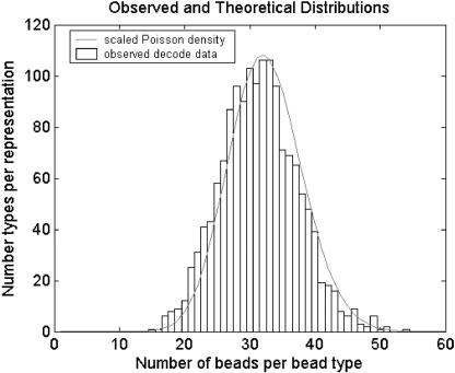
Bead representation histogram from a representative decoded array overlaid with a scaled Poisson density function. The loading of each array is a sampling of beads from a near infinite bead pool. Almost N ∼ 50,000 beads are sampled, and the probability, p, that a sampled bead belongs to a particular type is approximately one divided by the number of bead types. Because N is large, p is small, and the initial bead pool is near infinite, the number of beads from each bead type is well modeled by a Poisson distribution with mean Np. With 1520 bead types, we average >30 replicate beads per bead type, and the probability that any bead type has fewer than five replicate beads is extremely low (∼5.5 × 10⁻⁶).
A fundamental difference between randomly assembled arrays and conventional ordered arrays is that the number of beads (or probes) of each type is intrinsically a random variable with a Poisson sampling distribution for the former (Fig. 4) and is fixed and defined for the latter. Each randomly assembled array is effectively unique, having different numbers and arrangements of beads from array to array yet decoded by a single universal process. This notion is accepted for “liquid arrays” (Fulton et al. 1997), but is fairly radical in the field of spatially fixed microarrays. Nevertheless, the advantage of having multiple beads of each type is that the analytical assay precision is increased by both outlier removal and averaging of replicates (using subsampling of 1 to 20 beads (N) per bead type indicate that the extracted data conform to the theoretical rule of the error of the mean decreasing as  ; P. Ng, pers. comm.). At the same time, the random distribution of beads minimizes the chance of any local problem affecting the overall result, increasing robustness of the system. The only added requirement of using “unique” arrays is that the analytical data extraction step must use a uniquely defined template for each particular array. This was easy to implement as part of our data extraction software.
DISCUSSION
Our work provides a high-performance alternative to conventional microarrays. It also expands the reach of microarray assays. For example, we have used a highly miniaturized array format to construct a 96-array matrix for processing many microarray experiments cost-effectively, for ∼1500 assays at a time. This provides much needed statistical power that is difficult and prohibitively expensive to obtain by using conventional microarrays, and has the potential to speed the transition of microarray-based assays to large-scale clinical application.
We have used decoded arrays to create new assays for largescale genotyping (Fan et al. 2003) and gene expression (Yeakley et al. 2002; Fan et al. 2004) using a universal array format. We have also developed gene-specific probe sets for gene expression, and demonstrated limits of detection, precision, and dynamic range that are similar or superior to those obtained with conventional microarrays (M. Chee, K. Kuhn, S. Baker, and T. McDaniel, pers. comm.). Therefore, the technology is versatile and capable of conducting all the types of assays that are currently read out on conventional microarrays. For example, a wide variety of alternative genotyping assays could in principle be implemented on our platform (Gerry et al. 1999; Pastinen et al. 2000; Hardenbol et al. 2003). As a result, this work provides the foundation for a host of important existing applications in genomics, as well as new applications that are under development. Our technology is particularly effective at making large numbers of arrays of a given type, and is complementary to microarray technologies that are useful for screening large amounts of sequence with relatively few arrays (Chee et al. 1996; Patil et al. 2001; Nuwaysir et al. 2002).
Importantly, our technology has been proven in highly demanding and competitive large-scale genomics applications, in particular SNP genotyping (Fan et al. 2003). For example, the majority of the genotyping being carried out for the International HapMap Project, which aims to create a detailed map of common genetic variation across the human genome, is being carried out by using randomly assembled arrays manufactured by our decoding process, in conjunction with a new highly multiplexed genotyping assay that we also developed (Fan et al. 2003). The genotypes we have generated for the HapMap project are publicly available (www.hapmap.org). We routinely achieve a combination of call rates of >99.9% together with accuracy of 99.7% to 99.9%, with a capacity to process over a million genotypes per day that is scalable to much higher levels (Fan et al. 2003).
Random arrays have been particularly useful for the accurate, high-throughput, and cost-effective analysis of large numbers of samples for ∼1500 assays at a time, a need that was not met by conventional arrays. However, if random arrays are to realize their full potential, the capacity of the decoding scheme must be increased to allow the analysis of 10s or 100s of 1000s of assays per sample. Our approach to decoding is flexible and scalable. We have used a single decode sequence per bead, which works well for decoding 1000s of bead types. The decoding of 100,000s of bead types by the current process would require the synthesis of 100,000s of fluorescently labeled decoder oligos—an expensive and time consuming task. This bottleneck can be overcome by using multiple decoding sequences on each bead type such that if pairs of sequences are used, up to 106 (1000 × 1000) unique combinatoric sequences can be formed from just 2000 primary decoder sequences. By using this combinatoric approach, the decoder pools would only contain a complexity of 1000 to 2000 different sequences rather than 106 sequences.
Finally, the decoding algorithm is general and can, in principle, be applied to any spatially fixed collection of objects or molecules that are associated with specific DNA sequences. In genomics, the classification and characterization of large collections of sequences is often a key step in the analysis of complex biological systems. For example, a library of DNA clones is traditionally searched for a single gene of interest by hybridization to a labeled DNA probe (Sambrook 1989). The approach described here would allow a search for 1000s of genes at a time, while distinguishing closely related members of gene families and perhaps alternative splice forms. Similarly, electrophoretic separations of complex mixtures of nucleic acids are often probed to characterize a gene or its mRNA (Southern 1975; Alwine et al. 1979; Liang and Pardee 1992); this can also be parallelized. Finally, fluorescence in situ hybridization (FISH), a powerful class of methods with many applications, could be applied to 1000s of genes simultaneously. To illustrate, FISH with combinatorially labeled oligonucleotide probes has been used to measure transcription from 10 genes in a single cell (Levsky et al. 2002). The decoding strategy we describe could potentially allow transcription to be measured for all genes in a single cell.
In conclusion, we have developed a new and scalable way to make a novel type of microarray. The highly miniaturized arrays have performed well in a variety of applications. The decoding approach used to make them is both accurate and robust and can, in principle, be used to identify not only DNA sequences on beads but also other collections of DNA sequences.
METHODS
Preparation of Oligonucleotide-Linked Beads and Bead Pools
A set of 1536 universal capture oligonucleotide sequences was synthesized. Each sequence was individually immobilized on activated beads, as follows, to create 1536 bead types. Silica beads ∼3 μm in diameter (Bangs Laboratories, Inc.) were amino functionalized by incubation in 2.5% 3-amino-propyl-trimethoxysilane (Aldrich) in ethanol for 1 h at RT and then activated by reaction with 2% 2,4,6-trichloro-1,3,5-triazine (Aldrich) in acetonitrile for 2 h at room temperature. Synthetic oligonucleotides labeled at the 5′ terminus with a primary amine were covalently attached to the activated beads by overnight reaction at 50°C in a solution of 3 M NaCl and 100 mM sodium carbonate (pH 11). All reagents were of highest purity grade. Empirical measurements indicated that, on average, each bead carried on the order of 106 oligonucleotides. Following quality assessment, 16 of the bead types were discarded due to low signal-to-noise ratios. The remaining bead types were combined to create a pool containing 1520 functional bead types, each representing a unique capture sequence. The sequences were designed to serve as noninteracting decodable address sequences in addition to their function as probes that capture assay products from solution. They were selected to be 22 to 24 bases long with minimal cross-complementarity, similar GC content and Tm, no runs of a single base longer than five, and low similarity to human genomic sequences.
Preparation of Oligonucleotides and Pools Used in the Decode Process
Three sets of 1520 oligonucleotides complementary to the bead sequences were synthesized (Illumina Oligator synthesis). One set was unlabeled (corresponding to the OFF state), another with FAM, and a third with Cy3. The dye labels were incorporated during oligonucleotide synthesis by using 5′ phosphoramidites (Trilink Biotechnologies). After synthesis and deprotection, each oligonucleotide type was individually purified by using 96-well reverse-phase cartridge purification to yield labeled products >75% in purity. These sets of oligonucleotides were used to create eight unique decode pools, according to the strategy described below. Each pool contained 1520 decode sequences, each at a concentration of 10 nM.
Design of Decoder Pools
The strategy for the design of decoder pools to enable error checking, described in the main text, included the condition that all valid codes have exactly two OFF states, which allows for a maximum of 1792 codes. To enable the decoding of more bead types, we pooled the decoders so that valid codes have either exactly two OFF states or exactly five OFF states. The transition events that lead to misclassification are the same as described above, except that errors of the type (ON to OFF) or (OFF to ON) occurring in three different stages could also lead to a misclassification event. Three errors from ON to OFF could occur if a bead falls out of the array in the middle of decoding. To eliminate this source of error, all codes ending in three or more OFF states were removed from the set of valid codes. Finally, we eliminated any codes that do not have at least one ON state in each of the color channels that we use. The fact that each bead must show specific signal in two color channels during the decode process provides an additional quality check. The total number of valid color codes in this scheme is 2012.
Assembly of Array Matrices
Array matrices were manufactured in the following way: 96 optical fiber bundles were set in a rigid frame, in an 8 × 12 matrix that matches the layout of a standard 96-well microtiter plate. Each ∼1.4-mm-diameter hexagonally packed bundle contains 49,777 individual glass optical fibers fused together into a monolithic unit. The bundles were polished at both ends to a tolerance of ∼1 μm planarity across the entire matrix. One end served as the imaging surface and was used for the collection of fluorescence intensity data. The opposite end was etched in weak acid to create a well ∼3 μm in diameter at the end of each optical fiber. The fiber bundles were loaded by pipetting ∼0.4 μL (0.12 mg) beads in ethanol onto the end of each bundle, allowing the ethanol to evaporate, and removing excess beads. The assembled arrays were quite stable. Following eight stages of decoding and an overnight analytical hybridization (high salt at 48°C to 55°C), bead retention was typically >97%.
Decoding
Following bead assembly, arrays were hybridized to pools of 1520 decoders, each at 10 nM in decode buffer (600 mM NaCl, 60 mM potassium phosphate, 0.06% Tween-20, and 40% formamide at pH 7.6), for 12 min at room temperature. Following hybridization, three 1-min washes in wash buffer (167 mM NaCl, 16.7 mM potassium phosphate, 0.017% Tween-20 at pH 7.6) were used to remove unbound oligonucleotides. The arrays were then imaged at 1.0-μm resolution by using a 12-bit, 2000 × 3000-pixel CCD camera (Quantix 36E, Roper Scientific) and a standard achromatic 0.3 NA microscope imaging objective (field of view [FOV] = 2 mm) in a custom-engineered high-throughput imaging system (Barker et al. 2003). The imaging system uses an X, Y, Z stage assembly and positioning and autofocus software to collect images from all 96 arrays of a Sentrix array matrix automatically. Fluorescence excitation was performed by using a 300-W xenon arc lamp (ILC technology) and appropriate emission/dichroic/excitation filter sets. The FAM and Cy3 color channels were imaged separately. The light intensity at the sample was ∼20 to 35 mW. This imaging design minimizes spectral cross-talk between dyes because excitation and emission are done on peak. After imaging, the arrays were dehybridized by dipping into 0.1 N NaOH for 1 min and were then neutralized in decode buffer. The process of hybridization, washing, image collection, and dehybridization was carried out until eight hybridization stages were completed. The arrays were washed in water and ethanol, dried in nitrogen, and sealed with desiccant in a foil package.
Image Processing and Data Extraction
A core corresponds to an etched well in the optical fiber bundle and has a high probability of containing a bead. We developed algorithms and custom image processing software to discover the locations of cores in decode images and extract intensity data from them (Galinsky 2003a,b). The software identified, aligned, and indexed the cores in a process termed registration. The shift, rotation, and scale of each image were determined relative to a template image as part of this process. After registration, the core indices and locations were matched across the set of decode images. Intensity information for each core was then obtained by averaging a three-by-three-pixel region centered on the core. The diameter of each core is approximately three microns, and each pixel is a one micron square. Many 1000s of decoding images are collected in a day in the production facility. Thus, an automated image analysis pipeline was created to facilitate high-throughput processing.
Decoding Algorithms
We describe two algorithms used to assign decode signatures to beads. The first is called stage-by-stage decoding. In this approach, an intensity histogram is computed for each color channel of each decode stage. The histogram is bimodal because each stage and color channel will have beads that are in the ON state and beads that are in the OFF state. An intensity value that separates the ON state from the OFF state is chosen, and all cores are assigned a zero or one, depending on whether their intensity value is less than or greater than the separation threshold. The values assigned for each stage and color channel are combined into the decode signature. This algorithm is highly effective when the OFF state population is well separated from the ON state population. Further, the method is insensitive to shifts caused by stage-to-stage variability in intensity.
Pseudocode for Stage-by-Stage Decoding
For each stage do
For each color channel do
Input the N core intensity values.
Compute intensity histogram using 100 bins.
Locate the bin with the maximum height peak within the first 25 bins, and the bin with the maximum height peak within the last 75 bins.
Find the bin with the minimum height peak between the two maxima.
Determine C, the median intensity of the minimum height peak.
Label all cores with intensity lower than C with zero, and all cores with intensity greater than C as one.
Tabulate the zero and one stage and color information into the decode signatures.
The second algorithm is called core-by-core decoding. For each bead and color channel, we consider the eight intensity values across decode stages. The values are sorted, and the greatest relative intensity increase is determined. This is the separation between the ON and OFF states for the core. The same procedure is repeated for all beads in both color channels. The results are combined to give the decode signatures.
Pseudocode for Core-by-Core Decoding
For each core do
For each color channel do
Input the m intensity values for the core and color channel across stages.
Let I1 ... Im be the sorted intensity values.
Let Jk = (Ik+1 - Ik)/Ik, k = 1... m - 1 be the relative intensity jump from stage k to stage k + 1.
If the greatest relative jump occurs between stage K and K + 1, then assign zero to the core in stages 1... K, and assign one to the core in stages K + 1... m.
Tabulate the zero and one core and color information into the decode signatures.
The two methods give virtually identical results. In practice, we use the core-by-core method to decode the arrays, and obtain quality control information from the histograms. As part of the decoding process, quantitative metrics for array quality are output automatically and can be stored in a database. All processing and quality metric generation takes ∼20 min on a standard personal computer for a matrix of 96 arrays.
Estimation of Misclassification Rate
There are 1792 eight-stage color codes that have exactly two OFF states. A subset of these codes, (e.g., 1520) can be randomly selected and used in the design of decoder pools. The remaining 272 codes are unused. If a bead is misclassified (identified as the wrong bead type), the error cannot be observed because the number of beads of each type is random. However, because the used and unused color codes have the same form and are partitioned randomly, the number of beads that decode to unused color codes can be used to estimate the random misclassification rate. The estimate is given by [Bunused/(Bused + Bunused)] × [(Cused - 1)/Cunused], where Bi is the number of beads decoding to category i and Ciis the total number of color codes in category i. In other words, the estimate is the relative number of beads decoding to unused codes scaled by the ratio of the number of codes in the used and unused categories. In the current example, Cused = 1520 and Cunused = 272, but the computation is analogous for any other decode space design.
Acknowledgments
We are grateful to our Illumina colleagues in array manufacturing, process development, and engineering for invaluable technical assistance, and to Bob Kain and David Barker for numerous helpful discussions and insights. This work was supported in part by National Institutes of Health grants R44 HG02003-01, R21 HG01911, and R43 CA81952 to M.S.C.
The publication costs of this article were defrayed in part by payment of page charges. This article must therefore be hereby marked “advertisement” in accordance with 18 USC section 1734 solely to indicate this fact.
Article and publication are at http://www.genome.org/cgi/doi/10.1101/gr.2255804. Article published online before print in April 2004.
References
- Alwine, J.C., Kemp, D.J., Parker, B.A., Reiser, J., Renart, J., Stark, G.R., and Wahl, G.M. 1979. Detection of specific RNAs or specific fragments of DNA by fractionation in gels and transfer to diazobenzyloxymethyl paper. Methods Enzymol. 68: 220-242. [DOI] [PubMed] [Google Scholar]
- Barker, D.L., Therault, G., Che, D., Dickinson, T., Shen, R., and Kain, R. 2003. Self-assembled random arrays: High-performance imaging and genomics applications on a high-density microarray platform. Proc. SPIE 4966: 1-11. [Google Scholar]
- Battaglia, C., Salani, G., Consolandi, C., Bernardi, L.R., and De Bellis, G. 2000. Analysis of DNA microarrays by non-destructive fluorescent staining using SYBR green II. Biotechniques 29: 78-81. [DOI] [PubMed] [Google Scholar]
- Braeckmans, K., De Smedt, S.C., Leblans, M., Pauwels, R., and Demeester, J. 2002. Encoding microcarriers: Present and future technologies. Nat. Rev. Drug Discov. 1: 447-456. [DOI] [PubMed] [Google Scholar]
- Brenner, S., Johnson, M., Bridgham, J., Golda, G., Lloyd, D.H., Johnson, D., Luo, S., McCurdy, S., Foy, M., Ewan, M., et al. 2000. Gene expression analysis by massively parallel signature sequencing (MPSS) on microbead arrays. Nat. Biotechnol. 18: 630-634. [DOI] [PubMed] [Google Scholar]
- Chan, W.C., Maxwell, D.J., Gao, X., Bailey, R.E., Han, M., and Nie, S. 2002. Luminescent quantum dots for multiplexed biological detection and imaging. Curr. Opin. Biotechnol. 13: 40-46. [DOI] [PubMed] [Google Scholar]
- Chee, M., Yang, R., Hubbell, E., Berno, A., Huang, X.C., Stern, D., Winkler, J., Lockhart, D.J., Morris, M.S., and Fodor, S.P. 1996. Accessing genetic information with high-density DNA arrays. Science 274: 610-614. [DOI] [PubMed] [Google Scholar]
- Drmanac, S., Stavropoulos, N.A., Labat, I., Vonau, J., Hauser, B., Soares, M.B., and Drmanac, R. 1996. Gene-representing cDNA clusters defined by hybridization of 57,419 clones from infant brain libraries with short oligonucleotide probes. Genomics 37: 29-40. [DOI] [PubMed] [Google Scholar]
- Drmanac, S., Kita, D., Labat, I., Hauser, B., Schmidt, C., Burczak, J.D., and Drmanac, R. 1998. Accurate sequencing by hybridization for DNA diagnostics and individual genomics. Nat. Biotechnol. 16: 54-58. [DOI] [PubMed] [Google Scholar]
- Fan, J.-B., Oliphant, A., Shen, R., Kermani, B.G., Garcia, F., Gunderson, K.L., Hansen, M., Steemers, F., Butler, S.L., Deloukas, P., et al. 2003. Highly parallel SNP genotyping. Cold Spring Harbor Symp. Biol. 68: (in press). [DOI] [PubMed]
- Fan, J-B., Yeakley, J.M., Bibikova, M., Chudin, E., Wickham, E., Chen, J., Doucet, D., Rigault, P., Zhang, B., Shen, R., et al. 2004. A versatile assay for high-throughput gene expression profiling on universal array matrices. Genome Res. (this issue). [DOI] [PMC free article] [PubMed]
- Fodor, S.P.A., Read, J.L., Pirrung, M.C., Stryer, L., Lu, A.T., and Solas, D. 1991. Light-directed, spatially addressable parallel chemical synthesis. Science 251: 767-773. [DOI] [PubMed] [Google Scholar]
- Fulton, R.J., McDade, R.L., Smith, P.L., Kienker, L.J., and Kettman Jr., J.R. 1997. Advanced multiplexed analysis with the FlowMetrix system. Clin. Chem. 43: 1749-1756. [PubMed] [Google Scholar]
- Galinsky, V.L. 2003a. Automatic registration of microarray images, I: Rectangular grid. Bioinformatics 19: 1824-1831. [DOI] [PubMed] [Google Scholar]
- ———. 2003b. Automatic registration of microarray images, II: Hexagonal grid. Bioinformatics 19: 1832-1836. [DOI] [PubMed] [Google Scholar]
- Gerry, N.P., Witowski, N.E., Day, J., Hammer, R.P., Barany, G., and Barany, F. 1999. Universal DNA microarray method for multiplex detection of low abundance point mutations. J. Mol. Biol. 292: 251-262. [DOI] [PubMed] [Google Scholar]
- Gunderson, K.L., Huang, X.C., Morris, M.S., Lipshutz, R.J., Lockhart, D.J., and Chee, M.S. 1998. Mutation detection by ligation to complete n-mer DNA arrays. Genome Res. 8: 1142-1153. [DOI] [PubMed] [Google Scholar]
- Hamming, R.W. 1986. Coding and information theory. Prentice-Hall, Inc., Englewood Cliffs, NJ.
- Han, M., Gao, X., Su, J.Z., and Nie, S. 2001. Quantum-dot-tagged microbeads for multiplexed optical coding of biomolecules. Nat. Biotechnol. 19: 631-635. [DOI] [PubMed] [Google Scholar]
- Hardenbol, P., Baner, J., Jain, M., Nilsson, M., Namsaraev, E.A., Karlin-Neumann, G.A., Fakhrai-Rad, H., Ronaghi, M., Willis, T.D., Landegren, U., et al. 2003. Multiplexed genotyping with sequence-tagged molecular inversion probes. Nat. Biotechnol. 21: 673-678. [DOI] [PubMed] [Google Scholar]
- Hessner, M.J., Wang, X., Khan, S., Meyer, L., Schlicht, M., Tackes, J., Datta, M.W., Jacob, H.J., and Ghosh, S. 2003. Use of a three-color cDNA microarray platform to measure and control support-bound probe for improved data quality and reproducibility. Nucleic Acids Res. 31: e60. [DOI] [PMC free article] [PubMed] [Google Scholar]
- Holloway, A.J., van Laar, R.K., Tothill, R.W., and Bowtell, D.D. 2002. Options available—from start to finish—for obtaining data from DNA microarrays II. Nat. Genet. 32(Suppl): 481-489. [DOI] [PubMed] [Google Scholar]
- Hubbell, E. and Pevzner, P.A. 1999. Fidelity probes for DNA arrays. Proc. Int. Conf. Intell. Syst. Mol. Biol. 113-117. [PubMed]
- Johnson, P.H., Walker, R.P., Jones, S.W., Stephens, K., Meurer, J., Zajchowski, D.A., Luke, M.M., Eeckman, F., Tan, Y., Wong, L., et al. 2002. Multiplex gene expression analysis for high-throughput drug discovery: Screening and analysis of compounds affecting genes overexpressed in cancer cells. Mol. Cancer Ther. 1: 1293-1304. [PubMed] [Google Scholar]
- Kennedy, G.C., Matsuzaki, H., Dong, S., Liu, W.M., Huang, J., Liu, G., Su, X., Cao, M., Chen, W., Zhang, J., et al. 2003. Large-scale genotyping of complex DNA. Nat. Biotechnol. 21: 1233-1237. [DOI] [PubMed] [Google Scholar]
- Levsky, J.M., Shenoy, S.M., Pezo, R.C., and Singer, R.H. 2002. Single-cell gene expression profiling. Science 297: 836-840. [DOI] [PubMed] [Google Scholar]
- Liang, P. and Pardee, A.B. 1992. Differential display of eukaryotic messenger RNA by means of the polymerase chain reaction. Science 257: 967-971. [DOI] [PubMed] [Google Scholar]
- Lockhart, D.J. and Trulson, M.O. 2001. Multiplex metallica. Nat. Biotechnol. 19: 1122-1123. [DOI] [PubMed] [Google Scholar]
- Lockhart, D.J. and Winzeler, E.A. 2000. Genomics, gene expression and DNA arrays. Nature 405: 827-836. [DOI] [PubMed] [Google Scholar]
- Lockhart, D.J., Dong, H., Byrne, M.C., Follettie, M.T., Gallo, M.V., Chee, M.S., Mittmann, M., Wang, C., Kobayashi, M., Horton, H., et al. 1996. Expression monitoring by hybridization to high-density oligonucleotide arrays. Nat. Biotechnol. 14: 1675-1680. [DOI] [PubMed] [Google Scholar]
- Michael, K.L., Taylor, L.C., Schultz, S.L., and Walt, D.R. 1998. Randomly ordered addressable high-density optical sensor arrays. Anal. Chem. 70: 1242-1248. [DOI] [PubMed] [Google Scholar]
- Nicewarner-Pena, S.R., Freeman, R.G., Reiss, B.D., He, L., Pena, D.J., Walton, I.D., Cromer, R., Keating, C.D., and Natan, M.J. 2001. Submicrometer metallic barcodes. Science 294: 137-141. [DOI] [PubMed] [Google Scholar]
- Nuwaysir, E.F., Huang, W., Albert, T.J., Singh, J., Nuwaysir, K., Pitas, A., Richmond, T., Gorski, T., Berg, J.P., Ballin, J., et al. 2002. Gene expression analysis using oligonucleotide arrays produced by maskless photolithography. Genome Res. 12: 1749-1755. [DOI] [PMC free article] [PubMed] [Google Scholar]
- Pastinen, T., Raitio, M., Lindroos, K., Tainola, P., Peltonen, L., and Syvanen, A.C. 2000. A system for specific, high-throughput genotyping by allele-specific primer extension on microarrays. Genome Res. 10: 1031-1042. [DOI] [PMC free article] [PubMed] [Google Scholar]
- Patil, N., Berno, A.J., Hinds, D.A., Barrett, W.A., Doshi, J.M., Hacker, C.R., Kautzer, C.R., Lee, D.H., Marjoribanks, C., McDonough, D.P., et al. 2001. Blocks of limited haplotype diversity revealed by high-resolution scanning of human chromosome 21. Science 294: 1719-1723. [DOI] [PubMed] [Google Scholar]
- Pease, A.C., Solas, D., Sullivan, E.J., Cronin, M.T., Holmes, C.P., and Fodor, S.P. 1994. Light-generated oligonucleotide arrays for rapid DNA sequence analysis. Proc. Natl. Acad. Sci. 91: 5022-5026. [DOI] [PMC free article] [PubMed] [Google Scholar]
- Sambrook, J.E.A. 1989. Molecular cloning: A laboratory manual. Cold Spring Harbor Laboratory Press, Cold Spring Harbor, NY.
- Schena, M., Shalon, D., Davis, R.W., and Brown, P.O. 1995. Quantitative monitoring of gene expression patterns with a complementary DNA microarray. Science 270: 467-470. [DOI] [PubMed] [Google Scholar]
- Sengupta, R. and Tompa, M. 2002. Quality control in manufacturing oligo arrays: A combinatorial design approach. J. Comput. Biol. 9: 1-22. [DOI] [PubMed] [Google Scholar]
- Shannon, C.E. 1948a. A mathematical theory of communication. Bell System Technical J. 27: 379-423. [Google Scholar]
- ———. 1948b. A mathematical theory of communication. Bell System Technical J. 27: 623-656. [Google Scholar]
- Shearstone, J.R., Allaire, N.E., Getman, M.E., and Perrin, S. 2002. Nondestructive quality control for microarray production. Biotechniques 32: 1051-1052, 1054, 1056-1057. [DOI] [PubMed] [Google Scholar]
- Southern, E., Maskos, U., and Elder, R. 1992. Analyzing and comparing nucleic acid sequences by hybridization to arrays of oligonucleotides: Evaluation using experimental models. Genomics 13: 1008-1017. [DOI] [PubMed] [Google Scholar]
- Southern, E.M. 1975. Detection of specific sequences among DNA fragments separated by gel electrophoresis. J. Mol. Biol. 98: 503-517. [DOI] [PubMed] [Google Scholar]
- Taylor, E., Cogdell, D., Coombes, K., Hu, L., Ramdas, L., Tabor, A., Hamilton, S., and Zhang, W. 2001. Sequence verification as quality-control step for production of cDNA microarrays. Biotechniques 31: 62-65. [DOI] [PubMed] [Google Scholar]
- Van't Veer, L.J., Dai, H., van de Vijver, M.J., He, Y.D., Hart, A.A., Mao, M., Peterse, H.L., van der Kooy, K., Marton, M.J., Witteveen, A.T., et al. 2002. Gene expression profiling predicts clinical outcome of breast cancer. Nature 415: 530-536. [DOI] [PubMed] [Google Scholar]
- Wang, D.G., Fan, J.-B., Siao, C.-J., Berno, A., Young, P., Sapolsky, R., Ghandour, G., Perkins, N., Winchester, E., Spencer, J., et al. 1998. Large-scale identification, mapping, and genotyping of single-nucleotide polymorphisms in the human genome. Science 280: 1077-1082. [DOI] [PubMed] [Google Scholar]
- Watson, J.D. and Crick, F.H.C. 1953. Molecular structure of nucleic acid: A structure for deoxyribose nucleic acid. Nature 171: 737-738. [DOI] [PubMed] [Google Scholar]
- Yeakley, J.M., Fan, J.B., Doucet, D., Luo, L., Wickham, E., Ye, Z., Chee, M.S., and Fu, X.D. 2002. Profiling alternative splicing on fiber-optic arrays. Nat. Biotechnol. 20: 353-358. [DOI] [PubMed] [Google Scholar]
- Yvert, G., Brem, R.B., Whittle, J., Akey, J.M., Foss, E., Smith, E.N., Mackelprang, R., and Kruglyak, L. 2003. Trans-acting regulatory variation in Saccharomyces cerevisiae and the role of transcription factors. Nat. Genet. 35: 57-64. [DOI] [PubMed] [Google Scholar]
WEB SITE REFERENCES
- www.hapmap.org; International HapMap Project.