ESTGenes: Alternative Splicing From ESTs in Ensembl

Abstract

We describe a novel algorithm for deriving the minimal set of nonredundant transcripts compatible with the splicing structure of a set of ESTs mapped on a genome. Sets of ESTs with compatible splicing are represented by a special type of graph. We describe the algorithms for building the graphs and for deriving the minimal set of transcripts from the graphs that are compatible with the evidence. These algorithms are part of the Ensembl automatic gene annotation system, and its results, using ESTs, are provided at www.ensembl.org as ESTgenes for the mosquito, Caenorhabditis briggsae, C. elegans, zebrafish, human, mouse, and rat genomes. Here we also report on the results of this method applied to the human and mouse genomes.

Alternative splicing is a very important mechanism to provide functional diversity as well as regulation of the expression of genes (Lopez 1998; Black 2000, 2003; Smith and Valcarcel 2000). It allows the production of functionally diverse polypeptides from a single gene, and it accounts for most of the protein complexity in the organism. It has been observed in nearly all metazoan organisms, and it is estimated to occur in 30% to 60% of human genes (Minorov et al. 1999; Brett et al. 2000; Kan et al. 2001; Lander et al. 2001; Modrek and Lee 2002). Expressed sequence tags (ESTs) provide an abundant source of information to study alternative splicing (for a review, see Modrek and Lee 2002). ESTs are single-pass reads obtained from either the 5′ or the 3′ end of a cDNA clone. They represent snapshots of the transcriptome in a given set of conditions and therefore are an essential piece of information in order to find all the possible transcripts generated by a given genome. Moreover, although ESTs are sequenced in a given set of cell conditions, they provide a random sampling of the expression, as they are not necessarily constrained to any particular group of gene families. On the other hand, as ESTs represent partial transcripts, they still need to be processed in order to obtain from them a more complete knowledge about the transcriptome. Reliable methods are needed that can extract this information, and they must be robust against the errors present in the EST data. Some of these errors can be compensated for by the high redundancy of the data set, whereas others require specific curation (Modrek and Lee 2002).

We present here a novel algorithm, the ClusterMerge algorithm, that links a set of ESTs mapped to the genome according to whether they have a redundant splicing structure and produce a minimal set of putative transcript variants that have nonequivalent splicing structure and are compatible with the EST evidence. The resulting transcripts produced from ESTs are the ESTGenes as shown in the Ensembl Web site (www.ensembl.org). The algorithm can be applied to ESTs, mRNAs, or a combination of both. Although we will mostly deal with ESTs, everything described here can be also applied to cDNAs aligned to the genome.

The ClusterMerge algorithm is applied to genomically aligned ESTs, for instance, individual entries from dbEST (Boguski et al. 1993) aligned to the genome sequence. As pointed out previously in Bouck et al. (1999), EST self-clustering methods present a number of problems. On the other hand, when the genomic sequence is of good quality, genome-based methods facilitate the description of alternative transcripts and paralogous genes, as well as the identification of the correct strandedness by checking the splice-site consensus sequence. Moreover, these methods help prevent chimeras and processed pseudogenes. An EST aligned to the genome defines a splicing structure, which we represent by a transcript object. This transcript has attached exon objects with coordinates derived from the alignment. These coordinates are the start and end of the exon in the genomic sequence. Moreover, each exon has a start and an end coordinate in the space of the EST sequence, which run from one to the length of the EST. Aligned cDNAs can be represented in the same fashion.

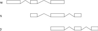
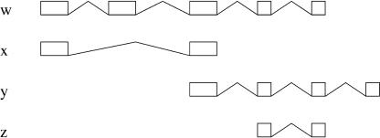
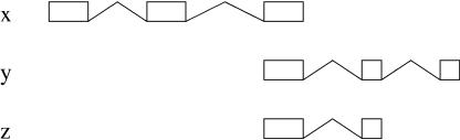
By using the genomic coordinates, we compare any two given ESTs, and this transcript comparison is used to define a criterion of redundancy. The simplest definition is to consider two ESTs to be redundant when they have a consecutive overlap of internal splice-sites and any other splice-site does not overlap the genomic extent of the other EST (Fig. 1). We then say that these two ESTs are mergeable; that is, they potentially represent two pieces of the same mRNA. The resulting transcript from this merge contains the union of all the introns from the two transcripts (Fig. 1).

Figure 1.

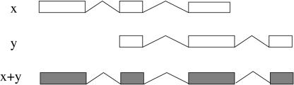
Merging ESTs. Two ESTs (x and y) can be considered in general to be mergeable if they have consecutive coincident splice-sites for the extent of the overlapping introns. The resulting merged EST (x + y) contains the union of all the introns from the two transcripts.

In this way we establish a relation between every pair of ESTs in a set. The problem is to find from these relations the maximal sets of compatible ESTs, and the number of sets must be minimal. Each one of these sets may contain enough information to reproduce the whole or part of the mRNA from which they are derived. Each set must be maximal in the sense that any other EST outside this set must have a splicing structure that is not compatible with at least one of the ESTs in the set. The resulting number of putative transcripts is minimal in the sense that if we remove one of the transcripts, there will be splicing structures in the EST set that cannot be accounted for.

Transcript Comparison and Merging Criteria

For efficiency, ESTs mapped to the genome are grouped into clusters in a first stage. This initial clustering is based on simple overlap of the genomic extent of the EST. The algorithm for grouping together mergeable ESTs is run on each of those clusters. At the heart of this algorithm is the comparison between two aligned ESTs (or cDNAs). The method to compare two transcripts (ESTs or cDNAs) is based on the genomic coordinates. A comparison returns one of these four possible values: non-overlap, clash, extension, or inclusion. A clash occurs when two ESTs overlap but their splicings are not compatible. Every pair of overlapping ESTs that have a compatible splicing structure can always be described as one of these two possibilities: inclusion or extension. An EST x includes an EST y if all internal splice-sites of y consecutively overlap with internal splice-sites of x. If a number of consecutive splice-sites in a prefix of an EST y overlap with a suffix of an EST x, we say that y extends x.

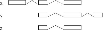
The definition of redundancy is independent of the actual algorithm linking the ESTs into mergeable sets. Indeed, the method to compare ESTs is independent of how the transcripts are combined. This makes the algorithm very flexible, as we can decide on our merging criteria independently of the construction of the redundant sets. We use three basic possible merging criteria (Fig. 2). The simplest one is when two ESTs have a consecutive overlap of internal splice-sites and no other splice-site overlapping the genomic extent of the other EST (case 1). For case 2 we relax the condition by allowing a certain mismatch at the exon boundaries. Finally, we consider also cases for which we bridge over tiny introns (case 3) in which small introns can be just the product of sequencing errors or misassemblies.

Figure 2.

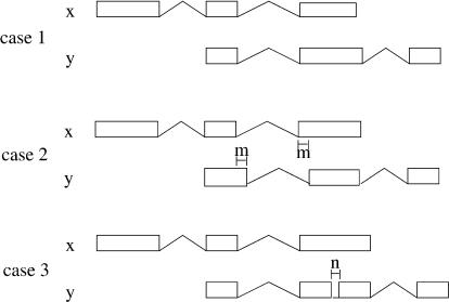
Criteria of merging. There are three basic forms of compatibility between two ESTs. In case 1, they have a consecutive overlap of internal splice-sites and no other splice-site that overlaps the genomic extent of the other EST. In case 2, we allow some mismatch of length ≤m at the exon boundaries. In case 3, we allow bridging over tiny introns of size ≤n. Thresholds m and n can be modified. In the ClusterMerge algorithm the comparison can be parameterized as a combination of these three basic cases.

The algorithm is parameterized on the compatibility criterion such that the user can choose either one of the above three possibilities or a combination of them. Moreover, we allow the user to input some values for the parameters shown in Figure 2. This is convenient to avoid splice variation artifacts introduced in the alignment by sequencing errors (this strategy was used in Modrek et al. [2001], allowing for a 6-bp variation). Another parameter, mentioned below, is the maximum number of base pairs that a terminal exon in an EST can overlap an intron in another EST, beyond which we do not merge the ESTs. This is used to model alternative 3′ ends, allowing for possible errors in the EST data. There is also a running mode in the algorithm for which the boundary mismatch is unconstrained. In this mode, the compatibility is simply defined as consecutive exon overlaps. Although we have observed that this is the best way to eliminate splice-site artifacts, it does not allow for alternative 5′/3′ splice-site prediction.

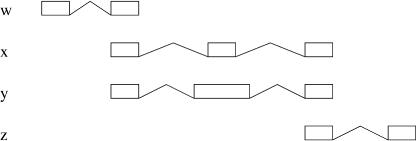
Our method is only based on the EST (or cDNA) evidence and will not try to predict missing exons or 5′/3′ ends of the transcripts if they are not present in the evidence. Kan et al. (2001) proposed a method for merging individual spliced introns so that spliced structures are created by chaining together sets of equivalent splice pairs. However, this method gives rise to structures that are not directly supported by any EST in the evidence (Fig. 3). A different method was proposed by Wheeler (2002). The method, however, has an exponential running time and includes an extension step that generates splice-site combinations that are not present in the EST evidence. In most of the cases, a combinatorial arrangement of the splice events produces splice variants that are not supported by the observed experimental evidence. Our method is different from others in that we exploit the nonlocal correlation between splice-sites to derive complete transcripts that have splice-sites compatible with the EST evidence (Fig. 3).

Figure 3.

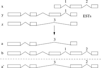
Extension versus nonextension. According to the evidence, splice-site 2 only appears together with splice-site 1. According to our logic of merging, sequence x can only merge with sequences that at least have splice-site 1 or 2, with the rest of the splice-sites either compatible or non-overlapping. In this case x can merge with y but not with z. To include splice-site 2 in transcript z, we would have to find in the evidence an EST with at least splice-sites 3 and 2. Our method therefore produces a and b from the available evidence and not a′. Other methods referred to in the text would sometimes produce a′ and b instead, trying to extend the transcript as much as possible, but this does not agree with the evidence.

METHODS

The Data Structure

In this section we describe the data structure underlying the algorithm. It is devised such that the numbers of comparisons necessary to build the different mergeable sets of ESTs (or cDNAs) are kept to a minimum. The information about the redundant splicing structure of ESTs can be efficiently represented as a graph. In this data structure, there is one node per EST, and the edges of the graph encode the redundancy relation between them. Every two overlapping ESTs that have a compatible splicing structure are related by either an inclusion or an extension relationship. An inclusion is represented in the graph by a double directed edge

and an extension by a single directed edge

Within each cluster of genomically aligned ESTs, we sort in two variables: by the 5′ end coordinate in ascending order, and if the 5′ coordinate is the same, by the 3′ coordinate in descending order. The inclusion relation is transitive, so we do not need to represent most of the edges in the graph. For example, the situation presented in Figure 4 corresponds to the graph

so we need not add an inclusion edge indicating the relation between x and z. The representation is similar for extensions, although in this case there is an ambiguity. For instance, the collection of ESTs given in Figure 5 is represented by the graph

We do not include an extension edge indicating the relation between w and y. Although this graph does not distinguish this case from the one in which there is no overlap between w and y, this is all we need to assert that they belong to the same mergeable set.

Figure 4.

Inclusion.

Figure 5.

Extension.

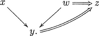
More complicated situations arise from the interaction of inclusions and extensions. For instance, if y extends x and z is included in both x and y as in Figure 6, our choice is the graph

where the relation between z and y can be recovered through x. Note that we locate inclusions as deep as possible in the graph, as formally defined below.

Figure 6.

Combination of inclusion and extension.

The subgraph defined by extension edges is not necessarily a tree. The example of Figure 7 is represented by a diamond-shaped graph

Figure 7.

Extensions giving rise to an acyclic graph.

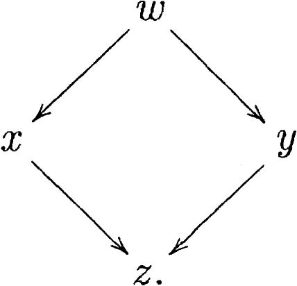Yet, the directed graph is always acyclic, a useful property exploited by the algorithm. We can obtain similar graphs with inclusion edges as well. The root of an inclusion subgraph can be thought of as the representative of all the nodes it includes as they have splicing structures that are redundant with respect to the root.

There are special cases in which inclusion branches can join. Take, for instance, Figure 8. If we only draw an inclusion edge from w to z, then the relation between x and z is lost. The solution is to compromise the simplicity of the representation by placing an inclusion edge from y to z:

Figure 8.

Configuration in which two inclusion edges to a node are preserved.

Observe that only drawing the edge from y to z is also inconvenient because any direct extension to w would miss its connection with z.

Formally, the edges present in the graph are defined by the following rules:

1. Given that y extends x, an extension edge x → y is present in the graph if there is no EST that extends x and is extended by y, and if there is no EST that includes x and is extended by y.

2. Given that x includes y, an inclusion edge x ⇒ y is present in the graph if there is no EST that includes y and is included by x, and if there exists no extension parent of x that does include y.

This data structure can be seen as an intertwined forest of inclusion and extension acyclic directed graphs. Henceforth, we refer to this structure as a ClusterMerge graph. Certain configurations are not possible in a graph of this kind. Two important examples are

In the left-hand graph, by rule 1 there must be a mismatch between z and x, but at the same time z is included in w, giving rise

to a contradiction. For the right-hand graph, y does not overlap with w (a mismatch is impossible here because x extends w and y is included in x), but z extends w and is included in y, which is contradictory. Actually, the only possible triangles in a graph of the type given above are of the form

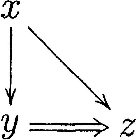which corresponds, for instance, to Figure 9. Thus, a triangle can be quickly verified in the vicinity of a node.

Figure 9.

Configuration giving rise to a triangle graph.

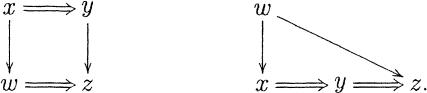
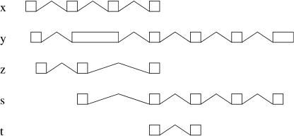
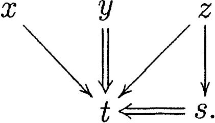
One of the advantages of this representation is that the mergeable sets can be recovered as special paths in the graph. We first define a leaf in a ClusterMerge graph to be a node that is not extended by any other node, and it is the root of an inclusion graph. Conversely, a root in a ClusterMerge graph is a node that does not extend any other node, although it can be an internal node in an inclusion graph. In the graph

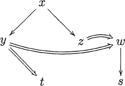the nodes x, t, and w are roots, and y, z and s are leaves. The graph above represents, for instance, the situation of Figure 10.

Figure 10.

Configuration with three graph roots.

A path in a ClusterMerge graph is a sequence of nodes obtained by following only extension edges. A collection of nodes in a path from a root to a leaf clearly gives a mergeable set. Moreover, to this set we can add for each node all the nodes in its inclusion subgraph; the resulting set is still mergeable and, in this case, maximal. For example, in the graph above the sets [x,y,w,t], [x,z,w], and [w,s] are the mergeable sets obtained in this manner.

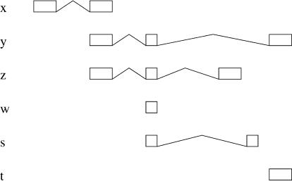
In some cases, mergeable sets can be unreachable, and then, the definition above is not fully satisfactory. Consider, for instance, Figure 11, the graph of which is

Figure 11.

Configuration with a mergeable set that does not include a leaf.

In this graph, y is both root and leaf. On the other hand, x and z are roots, whereas s is a leaf. The leaves give the mergeable sets [z,s,t] and [y,t], missing the other solution [t,x] (because t is not a leaf). In general, we say that a node is on the fringe of the graph when it is not extended. Observe that a path from a root to a node on the fringe represents a mergeable set, although not necessarily maximal. In the example above, the path from z to t returns a mergeable set that can be extended with s. On the other hand, the path from x to t represents our missing solution.

To include these solutions, we propose the following definition: Given a ClusterMerge graph, all the maximal mergeable sets are obtained as paths from a root to the fringe of the graph, where the last extension edge is not part of a triangle. As usual, for each node in the path, we must add all the nodes in the inclusion subgraph. Notice that if the node in the fringe is a leaf, then the last extension edge cannot be part of a triangle.

Building the Graph

In this section we describe the algorithm to build a ClusterMerge graph from a given set of ESTs. We first sort the transcripts by following the criteria mentioned above. Then the algorithm incrementally builds the graph by placing the next transcript into the graph containing the already analyzed ones. The ordering described above ensures a number of properties:

1. If an EST in the cluster does not overlap with a node in the graph, there will be no overlap with any other node in the same branch (i.e., in all the paths originating from any root).

2. When an EST w is included in another one y and overlaps with any of the ancestors in the extension branch or with any of the descendants in the inclusion subgraph of y, then w will necessarily extend or be included in y.

3. When an EST w clashes with a node x, w cannot be included in any of the ancestors in the extension branch of x or in any of the descendants in the inclusion subgraph of x. However, w could extend one of the elements in this inclusion subgraph.

In the implementation of a ClusterMerge graph, every node keeps a list of references to its extension parents and its inclusion children. This allows us to easily search the structure from the leaves to the roots in a bottom-up fashion. In this way, a ClusterMerge graph can be fully recovered from the list of its leaves. Observe that a graph is not necessarily connected, but this is not relevant to the algorithm or to the procedure to recover the mergeable sets described below.

The first EST in the list will always start the list of leaves L representing a trivial graph. The procedure follows by placing the next EST into the graph and updating the list of leaves. A new EST w is added to L if it becomes a leaf, and at the same time, those elements that are no longer leaves are removed. Extension branches can join and bifurcate, giving rise to very complex topologies; this requires strict discipline when searching the graph to ensure the new EST is placed in the correct position.

The algorithm is based on two mutually recursive methods. The method check-graph describes how we move along the leaves in the graph doing the comparisons between the new element and the ESTs already placed in the graph. From this method we call the method check-node, which, based on the result of the comparison, provides the decision logic for moving along the branches. The inclusion subgraph attached to a node q, represented by inclusion-graph(q) in the algorithm, is described by the list of the leaves obtained by removing the inclusion edges linking q with the first generation of inclusion children. The leaves of inclusion-graph (q) are defined as the nodes from the first inclusion-generation of q that are not extended. Further, we define an inclusion subgraph to be valid if there is at least one leaf in it. When performing the search via the method check-node, we apply check-graph on the inclusion subgraph of a node in a mutually recursive invocation.

As is usual in this kind of algorithm, we consider as a measure of complexity the number of comparisons necessary to build the corresponding graph. For a number N of ESTs, the algorithm for building a graph has a best running case linear in N, which happens, for instance, when each EST in the list extends the previous one. The worst running case is N², when every EST in the list clashes with all the others. The method check-graph is described here for a generic new element w and a generic graph T defined by the list of leaves L. When a new element is placed in the graph through an extension edge, we tag as “visited” the nodes in all the paths from the roots to the extension parents. The search over the graph is optimized by doing first a check on overlap (line 6). If w does not overlap the node, this will be skipped. Similarly, a node is skipped if it has been already visited (line 5). The actual results of the comparisons between transcripts are cached so that this result can be quickly retrieved when necessary. As soon as we find an extension in a graph, we place the new element, which becomes a new leaf of the graph. If the comparison returns a clash, we give priority to the inclusion-graph of the current node q if there exists a valid one. This recursively moves along the inclusion branch. By transitivity, the element w cannot be included in any node of the inclusion graph of q; that is, the only possibility of compatibility is the extension. Consequently, if w is placed, it becomes a new leaf of the main graph. If there is no valid inclusion-graph or we do not manage to place the new transcript in it, we then add the extension parents of the current node to the list of nodes to be checked. Thus, the algorithm performs a breadth-first search on the extension branches. Notice that if there is no overlap, we basically continue the search with the next element of the list L. Likewise, we return continue when a search in a graph has been exhausted without placing the new element. After each search, the nodes that stay as leaves, together with the new leaves, are put in L′ (line 7). Inclusions are handled by the method check-node. Within check-node, we call the method that does the actual comparison between two transcripts, compare (not shown here). If the result of the comparison is inclusion, a recursive search on the extension branches is triggered. This search stops as soon as we encounter an extension or a non-overlap case (line 7). Then the inclusion subgraph of the last node, say q, is verified (line 8). Because we are in the inclusion case, we know that the new element will be placed either in the current position or as one of the elements of inclusion-graph(q). In the next step, we verify whether it is placed in the inclusion graph; if not, we place it as inclusion child of q.

Furthermore, we add extension edges for each extension parent if necessary (line 10). Similarly, if q has no extension parents, we check its inclusion graph if there is any (line 12). If there is any inclusion-graph, we place w as included in q. Note that here we use the property that a clash is impossible after an inclusion. If the comparison results in something different from inclusion, we simply return that value (line 20), which will be dealt with in check-graph. On the other hand, if w was placed, then the value placed is returned so that the algorithm knows the recursion must be unwound, and then continue with the next leaf in the graph.

Recovering the Lists

Here we describe how to recover the mergeable sets from a ClusterMerge graph. As described previously, the paths along the extension branches from the roots to the leaves, collecting on each node the inclusion subgraph, produce maximal sets of compatible or mergeable elements. Because the extension branches in the graph can bifurcate and join, starting from one leaf we can recover more than one solution. The method solutions returns a list of sublists, each sublist being a solution derived from one of the paths along the extension branches. We recover all the solutions represented by the produced graphs by applying the method to each leaf. The method recursively follows the nodes in every extension branch (line 2). At each node it collects all the nodes in the inclusion subgraph only if the same subgraph is not also included in any of the extension parents (line 5). This avoids nodes being included twice for the special cases in which inclusion branches join (see graph 1.1). Every list of solutions S, which is a list of lists, is collected for every node (line 7) and returned. If there are no extension parents for a leaf, only the leaf plus the nodes in the inclusion subgraph are returned (line 8). When recovering the solutions, we also take into account those paths that run from a root to a node in the fringe of the graph for which the last extension is not a triangle (see graph 1.2). These special nodes are tagged as the graph is built, and the extension that gives rise to these special solutions is stored for those nodes. When recovering the solutions, if the node carries that tag, only the selected extension parents are used in line 1 of the method solutions. The method collect-inclusion-children (data not shown) in line 5 simply returns the node and its inclusion subgraph by recursively collecting each inclusion generation.

Merging the ESTs

Once we have collected the mergeable sets, from each set we derive a transcript with a splicing structure compatible with the evidence. To obtain this we cluster the exons in a list according to genomic overlap. Each exon cluster will contribute to a given exon in the final transcript. If the exon boundaries vary within the cluster, we take the most common coordinates for the 5′ and the 3′ ends. If the resulting exon produced from the cluster is going to become an internal exon in the final transcript, we do not allow external (5′ or 3′) ends of the exons in the cluster to contribute to the internal exon boundaries. For the case of exon boundaries that lie at the end of an EST and extend beyond an internal splice-site of another EST, we can parametrize how much overlap the external exon is allowed to have with the intron. When this parameter is zero, no overlap is allowed and the ESTs involved will not be merged; hence, we can model, for instance, a potential alternative UTR termination. Finally, for the exon clusters that contribute to the 5′ or 3′ terminal exons, and therefore are potential UTR exons, we choose the external coordinate from the evidence that would maximally extend the UTR.

From the resulting set of putative transcripts, we reject those that are unspliced, as they could be produced by spurious hits: They could be ESTs containing genomic sequence or be related to pseudogenes. On the other hand, such singletons might come from clusters representing a UTR region of a gene that had no overlap with a spliced EST. As we do not try to predict introns bridging incomplete clusters, this information is not used in the analysis. A possible solution to this problem was given in Kan et al. (2001).

Predicted transcripts and exons are stored in an Ensembl database. Each exon is linked to the ESTs that support it through the evidence table (Curwen et al. 2004). Likewise, each transcript can be linked to the ESTs that were used to build it. In this way, one could recover the sampling size for each one of the predictions by simply querying the database. This may be useful for establishing a confidence in the observations based on the sampling sizes, although it would require a careful analysis of the possible sampling bias (Kan et al. 2001). We use below the set of ESTs supporting each predicted transcript in a different way in order to assess the relilability of the exon structures.

Running the Algorithm

We have run the ClusterMerge algorithm for the human ESTs from dbEST (August 2003 version; Boguski et al. 1993) mapped to the human genome assembly version NCBI33 and for mouse ESTs from dbEST (same version) mapped to the mouse genome assembly version NCBI30. For both sets we clipped 20 bp on either end of each EST sequence and removed the remaining poly-A and poly-T tails. Only resulting sequences of at least 100 bp were kept. After this initial step, we were left with 4,945,605 human ESTs and 3,672,537 mouse ESTs. We used Exonerate (G. Slater, unpubl.) to produce the alignments. We divided the EST set into chunks and analyzed each chunk against each chromosome. We previously had masked the genomic sequence for repeats in libraries and low-complexity repeats. We used Exonerate with optimal options for speed, using an intron model like est_ genome (Mott 1997). From the resulting alignments, we rejected those with coverage and identity <97%. We took a best-in-genome approach, allowing for duplications if they had the same coverage. Furthermore, we rejected alignments for ESTs that were above the thresholds and unspliced, while having an spliced alignment elsewhere in the genome with a better coverage. This prevents the prediction of processed pseudogenes in the final set. In this way, 2,509,730 different human ESTs were mapped, forming 2,765,782 different genomic alignments. For mouse we mapped 1,879,238 different ESTs, forming 2,041,727 different genomic alignments.

We precomputed a set of chromosome pieces according to the density of ESTs, making the cuts in intergenic regions, to avoid any artificial splitting of the EST clusters. Before applying the ClusterMerge algorithm on these pieces, we performed some further filtering of the alignments. We rejected any EST that had intron splice-site dinucleotide sequences different from GT-AG, AT-AC, or GC-AG. For single-exon ESTs, we requested a minimum size of 200 bp and a minimum coverage of 99%. We rejected ESTs with introns <20 bp or >200 kb, or with exons <10 bp. We also checked that any insertion of the EST sequence in the alignment was not >2 bp. Furthermore, the ESTs aligned to the genomic sequence have been filtered according to their genomic length, keeping only those that have lengths equal to or greater than the median. Although the sequence length distribution of ESTs is approximate, the genomic length distribution is not. We therefore chose the media as better representative of these lengths. This filter is justified by the analysis of the results presented below and in Figures 12, 13, and 14. By using this stringent filtering, we expect to obtain a reliable set of predictions.

Figure 12.

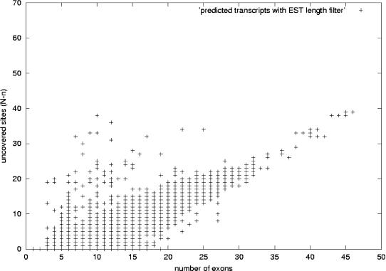
Uncovered sites versus number of exons for predicted human transcripts. This figure shows the distribution of predicted human transcripts. We have plotted the number of exons in the x-axis and in the y-axis the difference N-n: the difference between the number of sites of alternative splicing N in a transcript and the maximum number of consecutive sites n in that transcript covered by at least one EST. The value N-n is related to the confidence value described in the text, namely, confidence = 2^-(N-n). The plot corresponds to the set of 122,247 human transcripts predicted as described in the text: using a redundancy criterion that allows a mismatch of internal exon boundaries no >8 bp (case 2 in Fig. 2), and performing a genomic-length filtering on the ESTs. Transcripts along the y = 0 axis are those for which there are ESTs covering all the sites of alternative splicing. As the number of exons grows, N-n increases, as it is less likely to have ESTs covering all the exons in the transcript variant.

Figure 13.

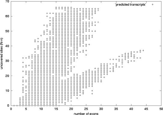
Predicted human transcripts without EST-genomic-length filtering. This figure shows the distribution of predicted human transcripts, with the number of exons in the x-axis and in the y-axis the difference N-n. In this case, the ESTs were not filtered according to their genomic length and the redundancy criterion used imposes exact matching for internal exon boundaries (case 1 in Fig. 2). These data are not described in the text and correspond to approximately double the number of transcripts plotted in Figure 12. As expected, N-n increases as the number of exons grows. In this case, there is a branch for which the difference N-n increases more rapidly with the number of exons and another branch for which this value increases in the same way as in Figure 12. We argue that on this plot, the set with faster growing N-n values is mainly produced by very short ESTs, which give rise to highly chimeric transcripts; hence, they are a less reliable set of trascript predictions. Comparing this figure with Figure 12 shows that by performing the genomic-length–based filtering and allowing some mismatch in the internal exon boundaries, we keep the good distribution of transcripts.

Figure 14.

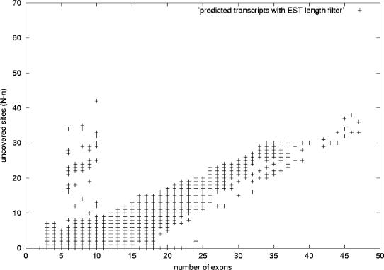
Uncovered sites versus number of exons for predicted mouse transcripts. This figure shows the distribution of mouse predicted transcripts. We have plotted the number of exons in the x-axis and in the y-axis the difference N-n: the difference between the number of sites of alternative splicing N the maximum number of consecutive sites n covered by at least one EST in a transcript. The plot corresponds to the set of 103,664 mouse transcripts predicted by using the same parameters as for the human case shown in Figure 12 and as described in the text: using a redundancy criterion that allows a mismatch of internal exon boundaries no >8bp (case 2 in Fig. 2), and performing a genomic-length filtering on the ESTs. Transcripts along the y = 0 axis are those for which there are ESTs covering all the sites of alternative splicing. As the number of exons grows, N-n increases, as it is less likely to have ESTs covering all the exons. The plot follows the same distribution as the human plot in Figure 12.

For every precomputed piece of genome, all the ESTs that passed the above filters are input to the algorithm. The running time varies depending on the number of ESTs in a given slice. The bulk of the computes are complete in ∼8 h using 200 CPUs, with few of the pieces taking much longer due to the high density of ESTs. For this test of the ClusterMerge algorithm, we used the redundancy criterion of allowing a mismatch at the exon boundaries of the ESTs not >8 bp (case 2 in Fig. 2), and we allowed any mismatch of external exons as long as these do not overlap an intron in another EST. For each transcript we predict an open reading frame (ORF): we take the longest ORF starting with ATG, and in the absence of ATG we simply take the longest one.

Validation of Human ESTGenes by Comparison With Mouse ESTGenes

We computed the ESTGene orthologs in the following way: Given a human ESTGene, we formed gene pairs by retrieving all the mouse ESTGenes located in a region homologous to the human region according to the human–mouse genomic alignments in the ensembl-compara database. Transcript variants from either gene in each gene pair were aligned with BLASTN (Altschul et al. 1997) by using default parameters. We considered only matches for which the alignment had no splits of size comparable to the smallest exon. The computed matches were filtered into pairs by using the alignment raw score and the same modified version of the stable marriage algorithm mentioned earlier for making an optimal set of pairs. Each pair was further checked to see that the exons aligned with each other when all of the genomic sequence (exons and introns) is considered. This is done to avoid homolog mutually exclusive exons being paired up as orthologs by the transcript alignment step. To this end, we took the genomic extensions of each transcript in human and mouse with 1000 bp of flaking sequence and realigned them using blastz (Schwartz et al. 2003). From the alignments, we checked that exon sequences were aligned with each other. We only kept the pairs that had a consecutive alignment of the exons in this way. We only considered ESTGene pairs for which there was at least one transcript pair with an alignment as described. This analysis yielded 18,242 human–mouse ESTGene pairs. The comparison is quite restrictive, so this represents a lower bound for the number of gene pairs. From these pairs, 984 ESTGenes were not in the Ensembl set for the human assembly NCBI33 and had a complete ORF.

RESULTS AND DISCUSSION

ESTGenes are currently being produced for the mosquito, C. briggsae, C. elegans, zebrafish, human, mouse, and rat genomes; the results can be viewed at www.ensembl.org. Each one of the possible transcripts within an ESTGene contains information about the ESTs that were used to build it. ESTGenes are also available in EnsMart (www.ensembl.org/EnsMart/; Kasprzyk et al. 2003), in which for the case of human they are also linked to the eVoc expression vocabularies (Kelso et al. 2003).

The ClusterMerge algorithm is also used with cDNAs as part of the Ensembl genebuild (Curwen et al. 2004). Species-specific cDNAs are aligned to the genome first, and then from those alignments, the minimal set of non-redundant transcripts is derived by using the methods presented in this article. This procedure helps eliminating redundancy in the cDNAs as well as solving possible fragmentation of the cDNA data. This set of putative transcripts is used in Ensembl to add possible alternative variants to the gene set predicted from protein evidence. This method has been used recently for the gene prediction in the rat genome by using rat and mouse cDNAs (the Rat Genome Sequencing Project Consortium 2004). ESTGenes are also used as evidence by the manual curators in the HAVANA group at the Sanger Institute (http://vega.sanger.ac.uk), where they are helpful to discern splice variants from EST information.

The Human and Mouse Transcriptomes

As a test case we have run the ClusterMerge algorithm for human and mouse using ESTs from dbEST (August 2003 version; Boguski et al. 1993). The details about the alignment procedure and how we run the ClusterMerge algorithm are given in Methods. The resulting number of predicted genes, transcripts, and exons is given in Table 1. The gff files with the human and mouse predictions can be found in the Supplemental material and in the Web site references. A 43% of the human ESTGenes and a 47% of mouse ESTGenes are alternatively spliced. Moreover, 42% of the predicted human transcripts and 36% of the predicted mouse transcripts had a complete ORF predicted in this way. In the following sections, we give detailed analysis of these results.

Table 1.

ESTGenes Predicted in Human and Mouse

	Human	Mouse
Genes	38,581	32,848
Transcripts	122,247	103,664
Exons	277,620	244,436

Comparison to Manually Annotated Genes

We carried out a comparison of the predicted ESTgenes in human with the manually annotated genes from chromosomes 6 (Mungall et al. 2003), 13 (A. Dunham, L.H. Matthews, J. Burton, J.L. Ashurst, K.L. Howe, K.J. Ashcroft, D.M. Beare, D.C. Burford, S.E. Hunt, S. Griffith-Jones, et al., in prep.), 14 (Heilig et al. 2003), and 20 (Deloukas et al. 2001) available at http://vega.sanger.ac.uk. We considered genes of type Known and Novel-CDS2 for the comparison. We looked at the gene, transcript, exon, and base-pair levels (see Tables 2, 3, 4, and 5). We note that a comparison like this is not entirely fair. EST information is by nature incomplete, and in our method, we do not actively try to predict complete gene structures beyond the available EST-sequence information. Moreover, genes annotated as Known and Novel-CDS are mainly based on full-length cDNAs and proteins; hence, the comparison is bound to yield low sensitivity values. Nevertheless, we can view the comparison as giving an idea of how much information is contained in the EST-data once it is processed to eliminate redundancy and increase transcript completeness, and how much potentially new information they can provide. An added difficulty in this comparison is that the manual annotation is based on an assembly different from NCBI33; hence, not all the annotation can be reliably transferred to this assembly. Thus, we carried out the comparison with the annotated genes that could be transferred: a total of 1844 Known and 572 Novel-CDS genes.

Table 2.

Gene and Transcript Level Comparison to Manual Annotations

	Gene Sn	Level Sp	Transcript Sn	Level Sp	No exons unpaired	1 exon unpaired	2 exons unpaired
chr13	0.82	0.39	0.71	0.42	35.6%	16.5%	10.7%
chr14	0.83	0.42	0.72	0.35	26.2%	17.5%	11.9%
chr20	0.85	0.46	0.64	0.45	32.2%	17.8%	11.6%
chr6	0.81	0.38	0.74	0.29	36.7%	16.3%	11.9%

Genes are compared according to the genomic extent, from which we draw gene pairs. At the transcript level, variants from either gene in the gene pairs are paired up according to the best transcript alignment. A transcript is considered as found if there is an alignment with a predicted transcript that has no better alignment with the other annotated transcripts. The sensitivity (Sn) is calculated as the number of paired-up annotated transcripts over the total number of annotated transcripts, and the specificity (Sp) is calculated by using the same numerator and the total number of predicted transcripts as denominator. We also give the percentage of the transcript pairs that have zero, one, and two exons unpaired.

Table 3.

Exact Exon Boundary Comparison to Manual Annotations

	Sn	Sp	Sn (coding)	Sp (coding)
chr13	0.35	0.38	0.52	0.48
chr14	0.38	0.36	0.57	0.44
chr20	0.34	0.34	0.51	0.46
chr6	0.39	0.30	0.51	0.40

All annotated exons are compared against all the predicted exons. An annotated exon is considered as found if there is at least one predicted exon with exact matching boundaries. The sensitivity (Sn) is calculated as the number of found exons over the total number of annotated exons, and the specificity (Sp) as the number of found exons over the total number of predicted exons. We carried out comparisons for all exons coding and noncoding (first two columns) and for coding exons only (last two columns).

Table 4.

Exon Level Per Transcript Pair Comparison to Manual Annotations

	Exact pairs	Sn	Sp	Exact pairs (coding)	Sn (coding)	Sp (coding)
chr13	61%	0.40	0.53	80%	0.45	0.75
chr14	64%	0.39	0.60	80%	0.41	0.79
chr20	62%	0.39	0.57	79%	0.43	0.76
chr6	61%	0.38	0.56	79%	0.42	0.75

Only exons that are part of a transcript pair are compared with each other. An annotated exon is considered as found it there is at least one predicted exon with exact matching boundaries in a given transcript pair. The second and fourth columns give the percentage of exact exon matches from the total number of exon pairs formed within the transcript pairs for all exons and for coding exons, respectively. The sensitivity (Sn) is computed as the number of exact exon matches within transcript pairs over the total number of annotated exons within transcript pairs. Similarly, the specificity (Sp) is computed as the number of exact exon matches within transcript pairs over the total number of predicted exons within transcript pairs. These values are given for coding exons only and for coding and noncoding exons together. The percentage of exact matches is higher when restricted to transcript pairs, and it is also higher for coding exons only. The specificity is much higher than in Table 3, and sensitivity is of comparable magnitude, which indicates that the predicted transcripts mostly miss exons rather than overpredict them. The high specificity also indicates that the transcript structures tend to agree with the annotations.

Table 5.

Base-Pair Level Comparisons to Manual Annotations

	Sn	Sp	Sn (coding)	Sp (coding)
chr13	0.46	0.70	0.55	0.75
chr14	0.50	0.68	0.58	0.72
chr20	0.47	0.69	0.58	0.69
chr6	0.50	0.60	0.56	0.64

We took the projections of the exon predictions and annotations over the genomic sequence and compare the overlap of both. The sensitivity (Sn) is calculated as the overlap length over the total extent of the annotation, whereas the specificity (Sp) is calculated as the overlap length over the total extent of the predictions. We give these values for coding regions only and for coding and noncoding regions together.

Currently, there are no standard statistical measures similar to those in Burset and Guigo (1996) for the prediction accuracy for cases of alternative splicing. Our case is special as there is abundant alternative splicing in both the annotations and the ESTGene predictions. We have tried to adapt some of the standard measures to our case. A gene was considered as found if its genomic extent had an overlap with at least one ESTGene. Transcripts within equivalent genes were paired up according to the best possible alignment of the exons: Each possible transcript pair is compared by using the exon coordinates, and a score is computed based on the extent of the overlap. The best pairs are computed then by using a symmetric version of the optimization method known as stable marriage (Gale and Shapely 1962; Irving et al. 1987) Every annotated transcript for which there was a predicted transcript paired up to it was considered as found. In Table 2 we also show the percentage of the transcript pairs that have zero, one, or two unpaired exons, disregarding the exon boundaries. For the comparison at the exon level (Table 3), an annotated exon was considered as found if there was at least one exon predicted that has the same exon boundaries.

Considering only the paired-up transcripts, we only look at the exon pairs that are within transcript pairs. In this context, we calculate two other measures (Table 4). One is the percentage of exact exon matches from the total number of exon pairs within each transcript pair. The other measure is the sensitivity and specificity of exact exon matches within the transcript pairs, which are calculated similarly to the previous case but restricted to the transcript pairs, so that an exon in a transcript is only compared to the exons in the corresponding transcript partner and not any other transcript. These two measures give more information about the accuracy of the predicted exon structure of the transcripts than the previous exon-level comparison. Finally, at the base-pair level (Table 5), the genomic extent of predicted nucleotides was compared to the genomic extent of the annotations.

As an extra test for the ESTGenes, we used pmatch (R. Durbin, unpubl.) to map the predicted peptides to the corresponding species set of SWISS-PROT (Boeckmann et al. 2003) and RefSeq (Pruitt et al. 2000) proteins (August 2003 version). For human we used 29,518 SWISS-PROT and 18,702 RefSeq proteins. From the predicted human set, 32,998 peptides in 16,514 different ESTGenes hit 16,642 RefSeq and 24,302 SWISS-PROT sequences. Moreover, there are 12,018 human ESTGenes with at least one complete ORF but with no hit on the known human protein set. We imply from here that the human proteome described by the ESTGenes has an ∼70% specificity. This value is higher than the one reported for the comparisons to annotations because there is no constraint to a genomic locus in the comparison; hence, a higher specificity means that many of the over-predictions in the comparison to the annotations in fact code for proteins similar to known genes. For mouse we used 28,881 SWISS-PROT and 15,670 RefSeq proteins. From the predicted mouse set, 29,073 peptides in 16,064 different ESTGenes hit 13,298 RefSeq and 23,478 SWISS-PROT sequences. Moreover, there are 8934 mouse ESTGenes with at least one complete ORF but with no hit at all on the known mouse protein set.

Comparison to the Ensembl Genes

By carrying out similar comparisons between the ESTGenes and the Ensembl genes for the human genome assembly NCBI33, we found 13,124 ESTGenes that are not in Ensembl. From those, 7873 have at least a complete ORF. On the other hand, we used the genomic alignments between human and mouse from the ensembl-compara database to obtain the subset of human EST-Genes that are conserved in mouse. From the 7873 ESTGenes not in the Ensembl set and with a complete ORF, there were 984 that we validated by finding a potential ortholog in the mouse EST-Gene set. The gff file with these predictions can be found in the Supplemental material and in the Web site references. The method to find these orthologs is described at the end of Methods. Note that all the transcripts involved are spliced and have canonical splice-site dinucleotides. These sets of predictions can be found in the Supplemental material.

Reliability of the Predictions

To analyze the reliability of the algorithm, we devised the following experiment. We considered all the RefSeq cDNAs that we could align to chromosome 20 by using the same method used for the ESTs (clipping the polyA tails but without clipping 20 bp at both ends), and mimicked a sampling of sequence tags by cutting them into random overlapping chunks. The overlap between the chunks was taken in the range between 20 and 60 nucleotides (nt), whereas the length of the chunks was taken between 300 and 600 nt. The cDNA data set consisted of 481 cDNAs aligned into 399 gene loci, in which 54 loci had more than one transcript. The ClusterMerge algorithm correctly recovered all the 345 single-transcript loci from the random chunks. From the 54 multi-transcript loci, five were correctly recovered without any missing or extra transcripts. These include the EYA2 locus with five variants (Fig. 15) and the WFDC2 locus with four variants. Further, there were nine loci with two variants such that both alignment structures were identical or one was completely included in the other, so the algorithm could make no distinction between the transcripts and only one transcript was generated. For only one of the 54 multi-transcript loci, the PANK2 locus (Fig. 16), two of the six variants present had the same alignment, so the algorithm did not separate them; the other four variants were correctly found.

Figure 15.

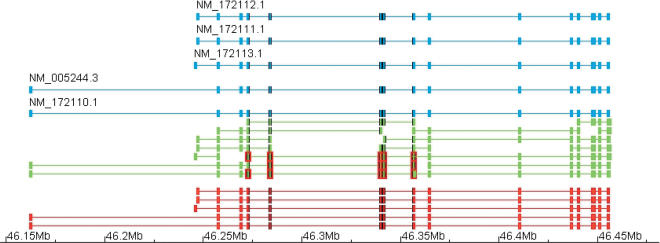
EYA2 gene locus. This figure shows the transcript predicted from the cDNA pieces on the EYA2 locus in chromosome 20. The aligned cDNAs are given in blue; the cDNA pieces, in green; and the predictions, in red. All the original cDNAs are recovered from the chunks. No chunk covered entirely any of the cDNAs. However, any two neighboring sites of alternative splicing were covered by at least one EST; hence, the global splicing information could be recovered by the algorithm. To improve clarity in the structure of the chunks, we have highlighted a set of those in the middle. Exons are highlighted in red and splice-sites in the original cDNAs, and the predicted transcripts are highlighted in black when they are coincident with the highlighted exons.

Figure 16.

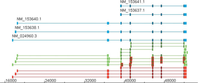
PANK2 gene locus. This figure shows the transcript predicted from the cDNA pieces on the PANK2 locus in chromosome 20. The aligned cDNAs are given in blue; the cDNA pieces, in green; and the predictions, in red. Two of the original cDNAs (NM_153637.1 and NM_153641.1) have exactly the same alignment; hence, they are merged into one by the algorithm. The algorithm recovered correctly all the non-redundant structures from the cDNA pieces. We have highlighted some of the chunks to improve the clarity of the structure of the chunks. The exons are highlighted in red, and the splice-sites of the cDNAs and the predicted transcripts are highlighted with a black line if they coincide with those exons.

For the nine remaining multi-transcript cases, we recovered all the variants but also predicted one or two extra ones, which were a chimeric combination of two of the original variants. This happened because the chunks were not long enough to cover two or more neighboring sites of alternative splicing. Accordingly, given two chunks from different cDNAs each covering a different site of alternative splicing, if they overlap on a constitutive exon, they will be combined by the algorithm, giving rise to a chimeric combination of alternative splices. Thus, we imply that there is a loss of global information about how alternative splices combine due to the sampling of cDNA chunks. These nine cases were further studied by using the overlap and the length of the chunks as variables, keeping one fixed while varying the other one in order to find thresholds at which we could recover the correct structures. We found that there is always a chunk length beyond which only those transcripts present in the original data set are generated, and this size correlates with the exon distance between the sites of alternative splicing. Moreover, below this threshold, regardless of the amount of overlap between the chunks, one or more extra chimeric transcripts are generated. For instance, for the case of the C20orf16 locus (Fig. 17), we had three cDNA RefSeqs aligned, which we could always correctly recover. However, for some combination of values for the chunk size and overlap, one extra chimeric transcript was generated. With an overlap of 40 nt and a piece length of ≥660 nt, no chimeric transcript was generated. This length is comparable to the exonic length separating both sites of alternative splicing; hence, information loss occurs when there is no sequence tag covering two consecutive sites of alternative splicing. As expected, the longer the ESTs, the more reliably we can recover the actual transcript structures. On the other hand, keeping the length of the pieces fixed at 640 nt, below the value for which the chimeric variant appears, and increasing the amount of overlap between the chunks up to >90% of their length, which also produces a larger amount of pieces, still generates the chimeric variant. Other cases in which chimeric transcripts appeared include the PTPRA and RASSF2 loci. These results indicate that a large depth of EST alignments may help confirming exons and splices, but it might not contain enough information to reliably recover the splicing structure of the transcript variants. Moreover, this justifies a filter for shorter ESTs, which are less likely to add any new information. The combination of the algorithm with other information sources, such as the 5′/3′ orientation of the EST or the clone name, can help recovering the actual structure; however, this information is not always available or complete.

Figure 17.

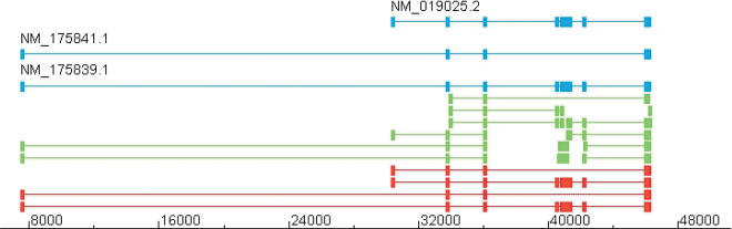
C20orf16 gene locus. This figure shows the transcript predicted from the cDNA pieces on the C20orf16 locus in chromosome 20. The aligned cDNAs are given in blue; the cDNA pieces, in green; and the predictions, in red. The three original cDNAs are correctly recovered from the chunks. However, one extra chimeric combination of chunks is produced: the uppermost of the predictions. This happens when the cDNA pieces do not cover two or more neighboring sites of alternative splicing.

The experiment described above suggests a way of assessing the reliability of the predicted transcript structures based on the coverage of sites of alternative splicing by ESTs. A set of predicted transcripts in a gene locus defines a set of sites of alternative splicing, which we derive by looking at the genomic positions of the exons and testing for cases of exon-skipping, alternative 5′/3′ site, mutually exclusive exons, or cassette exon. In an alternatively spliced gene, each transcript variant contains one or more of these sites. Consider the simplest case of two sites A and B. If there is no EST covering these two sites, assuming a binary event for each site, that is, A⁺ and A^-, the alternative splices will combine in a combinatorial fashion, producing four transcript structures, which we can represent as follows: A⁺ ⊗ B⁺, A⁺ ⊗ B^-, A^- ⊗ B⁺, and A^- ⊗ B^-. On the other hand, for a given observed splice event, for example, A⁺, considering the observed events in the other site, we can only be sure that one of the combinations is the correct one. The other one is not necessarily incorrect, but in terms of the information available, there is an increased chance that one of the combinations is chimeric. Accordingly, we can associate a confidence or reliability value to each transcript related to this uncertainty. For the present example we assign a confidence value 1/2 to each of the transcripts containing the splice event A⁺. Similarly, we assign a confidence value 1/2 to each transcript containing the splice event A^-. Intuitively, out of the four possible transcripts, we are certain about two of the predictions given the observed EST data, but we do not know which two; hence, the factor 1/2.

We extend this formalism to transcripts with three or more sites of alternative splicing and calculate for each transcript the reliability factor. We first calculate for a transcript the sites with alternative splice events relative to the other transcripts in the same gene locus. Assume the transcript has N sites. We then consider iteratively all the possible N - m + 1 combinations of m ≤ N neighboring sites starting at m = N, until we find the maximum n = m_max, for which there is at least an EST covering the n neighboring sites. We give to that transcript a confidence value of 2^-(N-n); that is, every step we decrease m, we multiply the confidence of the prediction by a factor 1/2. We can alternatively represent the reliability in terms of N-n: the difference between the number of sites in a transcript N and the maximal number of consecutive sites covered by at least one EST. In Figures 12 and 14, we give the plots of the distribution of predicted transcripts in human and mouse, showing the number of exons in each transcript against the value of N-n for the transcript. For comparison, in Figure 13 we show the same type of plot for the human but in which the predictions have been obtained by using different parameters for the algorithm (see legend for details).

Availability of the Software

The code for the ClusterMerge algorithm and all other analyses described in this article is part of the Ensembl software for computational genome analysis freely available from the cvs repository at www.ensembl.org. There is also a script, which can read in transcript data and produce the output in GFF format, at ensembl-pipeline/scripts/EST/cluster_merge.pl, that is more convenient for analyzing short pieces of a genome. The code for the algorithm, independent of the Ensembl API, is available at http://genome.imim.es/~eeyras.

Algorithm 1.

check-graph(node w, graph T)

1:	L ← leaves(T)
2:	L′ empty list
3:	whileL non-empty do
4:	q ← dequeue L
5:	skip q if `visited'
6:	case check-node(w, q):
	non-overlap⇒ add q to L′
	places ⇒ q ← queue L′ if q still leaf
	extension ⇒ place here — w ← queue L′
	tag extension-ancestors(w) as `visited'
	clash ⇒ check-graph(inclusion-graph (q))
	if not placed then
	extension-parents(q) ← queue L
	q ← queue L′
7:	leaves(T) ← L′
8:	ifw placed then
9:	return `placed'

Algorithm 2.

check-node(node w, node q)

1:	result1 = compare(w, q)
2:	ifresult1 = `inclusion' then
3:	if ∃ extension-parents(q) then
4:	for each p ∈ extension-parents (q) do
5:	skip node if `visited'
6:	result2 = check-node(w, extension-parent(q))
7:	ifresult2 = `extension' or `non-overlap' then
8:	check-graph(w, inclusion-graph (q))
9:	if w cannot be placed in inclusion-graph(q) or ∄ inclusion-graph(q)
10:	⇒ add the inclusion of w in q
11:	add extension to p if any
12:	else if ∃ valid inclusion-graph(q) then
13:	return check-graph(w, inclusion-graph(q))
14:	else
15:	place inclusion here
16:	else
17:	returnresult1
18:	ifw placed then
19:	return `placed'
20:	else
21:	returnresult1

Algorithm 3.

solutions(node y)

1:	for each p extension-parent of ydo
2:	S ← solutions(p)
3:	add y to each solution in S
4:	for each c inclusion-child of ydo
5:	collect-inclusion-children(c) if c not included in p
6:	add children to each solution in S
7:	collect S
8:	return all lists S if any or return collect-inclusion-children (y)

References

- Altschul, S., Madden, T., Schaffer, A., Zhang, J., Zhang, Z., Miller, W., and Lipman, D. 1997. Gapped BLAST and PSI-BLAST: A new generation of protein database search programs. Nucleic Acids Res. 25: 3389-3402. [DOI] [PMC free article] [PubMed] [Google Scholar]
- Black, D. 2000. Protein diversity from alternative splicing: A challenge for bioinformatics and post-genome biology. Cell 103: 367-370. [DOI] [PubMed] [Google Scholar]
- ———. 2003. Mechanisms of alternative pre-messenger RNA splicing. Annu. Rev. Biochem. 72: 291-336. [DOI] [PubMed] [Google Scholar]
- Boeckmann, B., Bairoch, A., Apweiler, R., Blatter, M. C., Estreicher, A., Gasteiger, E., Martin, M.J., Michoud, K., O'Donovan, C., Phan, I., et al. 2003. The SWISS-PROT protein knowledge base and its supplement TrEMBL in 2003. Nucleic Acids Res. 31: 365-370. [DOI] [PMC free article] [PubMed] [Google Scholar]
- Boguski, M., Lowe, T., and Tolstoshev, C. 1993. dbEST: Database for expressed sequence tags. Nat. Genet. 4: 332-333. [DOI] [PubMed] [Google Scholar]
- Bouck, J., Yu, W., Gibbs, R., and Worley, K. 1999. Comparison of gene indexing databases. Trends Genet. 15: 159-161. [DOI] [PubMed] [Google Scholar]
- Brett, D., Hanke, J., Lehmann, G., Haase, S., Delbruck, S., Krueger, S., Reich, J., and Bork, P. 2000. EST comparison indicates 38% of human mRNAs contain possible alternative splice forms. FEBS Lett 474: 83-86. [DOI] [PubMed] [Google Scholar]
- Burset, M. and Guigo, R. 1996. Evaluation of gene structure prediction programs. Genomics 34: 353-367. [DOI] [PubMed] [Google Scholar]
- Curwen, V., Eyras, E., Andrews, D.T., Clarke, L., Mongin, E., Searle, S., and Clamp, M. 2004. The Ensembl automatic gene annotation system. Genome Res. (this issue). [DOI] [PMC free article] [PubMed]
- Deloukas, P., Matthews, L.H., Ashurst, J., Burton, J., Gilbert, J.G., Jones, M., Stavrides, G., Almeida, J.P., Babbage, A.K., Bagguley, C.L., et al. 2001. The DNA sequence and comparative analysis of human chromosome 20. Nature 414: 865-871. [DOI] [PubMed] [Google Scholar]
- Gale, D. and Shapely, H. 1962. College admissions and the stability of marriage. Am. Math. Monthly 69: 9-15. [Google Scholar]
- Heilig, R., Eckenberg, R., Petit, J.-L., Fonknechten, N., Da Silva, C., Cattolico, L., Levy, M., Barbe, V., de Berardinis, V., Ureta-Vidal, A., et al. 2003. The DNA sequence and analysis of human chromosome 14. Nature 421: 601-607. [DOI] [PubMed] [Google Scholar]
- Irving, R., Leather, P., and Gusfield, D. 1987. An efficient algorithm for the optimal stable marriage. Journal of the Association for Computer Machinery 34: 532-544. [Google Scholar]
- Kan, Z., Rouchka, E., Gish, W., and States, D. 2001. Gene structure prediction and alternative splicing analysis using genomically aligned ESTs. Genome Res. 11: 889-900. [DOI] [PMC free article] [PubMed] [Google Scholar]
- Kasprzyk, A., Keefe, D., Smedley, D., London, D., Spooner, W., Melsopp, C., Hammond, M., Rocca-Serra, P., Cox, T., and Birney, E. 2003. EnsMart: A generic system for fast and flexible access to biological data. Genome Res.. 14: 160-169. [DOI] [PMC free article] [PubMed] [Google Scholar]
- Kelso, J., Visagie, J., Theiler, G., Christoffels, A., Bardien, S., Smedley, D., Otgaar, D., Greyling, G., Jongeneel, C., McCarthy, M., et al. 2003. eVOC: A controlled vocabulary for unifying gene expression data. Genome Res. 13: 1222-1230. [DOI] [PMC free article] [PubMed] [Google Scholar]
- Lander, E.S., Linton, L.M., Birren, B., Nusbaum, C., Zody, M.C., Baldwin, J., Devon, K., Dewar, K., Doyle, M., FitzHugh, W., et al. 2001. Initial sequencing and analysis of the human genome. Nature 409: 860-921. [DOI] [PubMed] [Google Scholar]
- Lopez, A. 1998. Alternative splicing of pre-mRNA: Developmental consequences and mechanisms of regulation. Annu. Rev. Genet. 32: 279-305. [DOI] [PubMed] [Google Scholar]
- Minorov, A., Fickett, J., and Gelfand, M. 1999. Frequent alternative splicing of human gene. Genome Res. 9: 1288-1293. [DOI] [PMC free article] [PubMed] [Google Scholar]
- Modrek, B. and Lee, C. 2002. A genomic view of alternative splicing. Nat. Genet 30: 13-19. [DOI] [PubMed] [Google Scholar]
- Modrek, B., Resch, A., Grasso, C., and Lee, C. 2001. Genome-wide detection of alternative splicing in expressed sequences of human genes. Nucleic Acids Res. 29: 2850-2859. [DOI] [PMC free article] [PubMed] [Google Scholar]
- Mott, R. 1997. EST_GENOME: A program to align spliced DNA sequences to unspliced genomic DNA. Comput. Appl. Biosci. 13: 477-478. [DOI] [PubMed] [Google Scholar]
- Mungall, A.J., Palmer, S.A., Sims, S.K., Edwards, C.A., Ashurst, J.L., Wilming, L., Jones, M.C., Horton, R., Hunt, S.E., Scott, C.E., et al. 2003. The DNA sequence and analysis of human chromosome 6. Nature 425: 805-811. [DOI] [PubMed] [Google Scholar]
- Pruitt, K.D., Katz, K.S., Sicotte, H., and Maglott, D.R. 2000. Introducing RefSeq and LocusLink: Curated human genome resources at the NCBI. Trends Genet. 16: 44-47. [DOI] [PubMed] [Google Scholar]
- Rat Genome Sequencing Project Consortium. 2004. Genome sequence of the Brown Norway rat yields insights into mammalian evolution. Nature 428: 493-521. [DOI] [PubMed] [Google Scholar]
- Schwartz, S., Kent, W.J., Smit, A., Zhang, Z., Baertsch, R., Hardisson, R.C., Haussler, D., and Miller, W. 2003. Human–mouse alignments with BLASTZ. Genome Res. 13: 103-107. [DOI] [PMC free article] [PubMed] [Google Scholar]
- Smith, C.W. and Valcarcel, J. 2000. Alternative pre-mRNA splicing: the logic of combinatorial control. TIBS 25: 381-388. [DOI] [PubMed] [Google Scholar]
- Wheeler, R. 2002. A method of consolidating and combining EST and mRNA alignments to a genome to enumerate supported splice variants. Lecture Notes in Computer Science 2452: 201-209. [Google Scholar]
WEB SITE REFERENCES
- http://vega.sanger.ac.uk/; manual annotations of human chromosomes.
- http://www.ensembl.org/EnsMart/; Ensmart start page.
- www.ensembl.org; The Ensembl Genome Browser
- http://genome.imim.es/~eeyras; The code for the algorithm is available in this Web page.