

Abstract
We draw on macroeconomic models of diffusion and productivity to explain empirical patterns of survival gains in heart attacks. Using Medicare data for 2.8 million patients during 1986–2004, we find that hospitals rapidly adopting cost-effective innovations such as beta blockers, aspirin, and reperfusion, had substantially better outcomes for their patients. Holding technology adoption constant, the marginal returns to spending were relatively modest. Hospitals increasing the pace of technology diffusion (“tigers”) experienced triple the survival gains compared to those with diminished rates (“tortoises”). In sum, small differences in the propensity to adopt effective technology lead to wide productivity differences across hospitals.
1. Introduction
There were large regional differences in per capita price-adjusted 2010 U.S. Medicare expenditures, ranging from $6,911 in Lacrosse, Wisconsin, to $13,824 in McAllen, Texas. Yet there is mixed evidence on whether more spending is associated with better outcomes (e.g., Fisher et al., 2003; Skinner et al., 2005; Doyle et al., 2011, 2014), and some have estimated the level of waste in health care spending equal to 3 percent of GDP or more (Cutler et al., 2013; Fisher et al., 2003a,b). This lack of association between spending and outcomes has sometimes been interpreted as “flat of the curve” health care spending, or variations along a common production function with a very low or zero marginal value of health care spending.1
The “flat of the curve” explanation is problematic for many reasons. Some studies find a negative association between state-level quality measures and per capita Medicare expenditures (Baicker and Chandra, 2004); why should spending more be associated with providing worse quality care? Second, given results from Cutler, et al. (1998), Berndt et al. (2002), and others that over time, survival and functioning has improved because of often expensive new medical technology, it would be surprising if the “wasted” health care spending equal to 3 percent of GDP should provide no benefit whatsoever.
In this paper, we draw on macroeconomic models of productivity to provide a better explanation for this empirical puzzle. That differential rates of technology adoption can explain long-term variations in per capita GDP across countries is by now well understood. Crespi, et al. (2008) found as much as 50 percent of total factor productivity growth arises simply from the flow of knowledge across firms. Parente and Prescott (1994, 2002) showed that surprisingly small differences in the rates of technological adoption could imply large disparities in country levels of income, while Eaton and Kortum (1999) estimated that countries realized just two-thirds of the potential productivity gains because of the slow diffusion and adoption of ideas across borders (see also Hall, 2004, Comin and Hobijn, 2010, and Comin and Mestieri, 2013).
There is a parallel literature in health care documenting similar lags in adoption, and with similar adverse effects on overall productivity. Despite powerful evidence from a 1601 experiment demonstrating the effectiveness of lemon juice in preventing scurvy, the British Navy did not require foods containing vitamin C until 1794 (Berwick, 2003).2 Similarly, beta blockers, drugs costing pennies per dose, were shown during the early 1980s to reduce mortality by as much as 25 percent following a heart attack (Yusuf, et al., 1985), yet by 2000/2001 median state-level use was still only 68 percent (Jencks, et al., 2003).
We develop a general model in which hospitals and physicians seek to maximize the health of their patients by adopting new technologies in the face of financial and knowledge-based barriers. Variation across hospitals in these barriers leads to differences in the diffusion rate of new technologies. We apply this model to the treatment of patients diagnosed with an acute myocardial infarction (AMI, or a heart attack) during the period 1986–2004, a period of particularly rapid diffusion for new technologies.
We first consider three types of innovations that are highly effective, and highly cost-effective, in saving lives following AMI: Aspirin, beta blockers, and reperfusion within 12 hours of the heart attack. (Reperfusion consists either of thrombolytic “clot-busting” drugs, or percutaneous coronary interventions (PCI), also known as angioplasty.)3 We also consider the diffusion of technology first introduced in 2003, drug-eluting stents, to identify how changes over time in the speed with which new (and valuable) hospital innovations diffuse affect health outcomes. Finally, we test whether hospitals adopting these three highly effective treatments also adopted other, less cost-effective technologies such as lidocaine, a drug with initially favorable results but whose effectiveness was questioned in the late 1980s, “late” surgical angioplasty (PCI) more than 24 hours after the AMI (again with less clear clinical effectiveness), and coronary artery bypass surgery (CABG).
The model is tested using a sample of 2.8 million heart attack patients drawn from the fee-for-service Medicare population during 1986–2004. Like Eaton and Kortum’s (1999) study of aggregate productivity, we find substantial differences in the extent to which some hospitals lag behind in the diffusion of highly effective technologies, and that this differential lag can explain a nearly 3 percentage point difference in one-year survival between rapid-diffusing and slow-diffusing hospitals, almost one-third of the overall improvement in outcomes during 1986–2004. These productivity effects swamp the influence of differences in factor inputs, a result also found in the macroeconomics literature (e.g., Hall and Jones, 1999). We demonstrate that the “Asian tiger” hospitals which between 1994/95 and 2003/04 demonstrated dramatic improvements in diffusion rates also experienced above-average survival growth, and three times the growth in the “tortoise” hospitals that experienced a decline in diffusion rates.
Finally, we found evidence that hospitals investing in highly effective medical innovations (aspirin, beta blockers, dropping the use of lidocaine) were quite different from those continuing the use of lidocaine and most notably adopting a mix of less cost-effective surgical innovations (early reperfusion, late PCI angioplasty, bypass surgery).4 Consistent with Hall (2014), the survival benefits arising from the more effective medical innovations are estimated to be larger than those arising from the second, less effective mix of treatments. This evidence suggests that barriers to the diffusion of knowledge about the effectiveness of new technologies play an important role in explaining productivity differences across hospitals, rather than barriers to the adoption of new technologies per se.
These results can potentially reconcile two seemingly divergent views of the U.S. health care system. Technological progress has led to dramatic improvements in survival for heart attack patients (as in Cutler, 2004), but these improvements are largely associated with the adoption of effective new technologies, rather than more factor inputs per se (Chandra and Skinner, 2012). Holding technology diffusion constant, however, we find modest improvements in outcomes associated with greater factor inputs, with a preferred estimate of between $94,000 and $155,000 per life-year. Chandra et al. (2013) found similar variation in productivity across firms in non-health industries as in hospitals, suggesting that the differences across firms in technology adoption may not be unique to health care. The real puzzle, therefore, is why many physicians and hospitals – and firms more generally – fail to adopt highly-efficient (or even modestly efficient) innovations.
2. The Model
We focus on the “production” of survival following acute myocardial infarction (AMI). There are compelling reasons to focus on heart attacks. Nearly every AMI patient who survives the initial attack is admitted to a hospital, and ambulance drivers generally take the patient to the nearest hospital (although see Doyle et al., 2014). The outcome, survival, is accurately measured and there is broad clinical agreement that survival is the most important endpoint, particularly in the elderly population. The measurement of inputs is also accurate, as is risk adjustment including the type of heart attack. Finally, many of the studies focusing on the value of medical technology have used AMI as an example (Cutler, et al., 1998; Cutler, 2004; Doyle, 2011).
The Hospital Production Function
We develop a simple model of hospital productivity that distinguishes between inputs that require substantial contributions of capital and labor (e.g., hospital bed-day or surgical procedures) and technology innovations where barriers are unlikely to arise solely from financial constraints. Suppose that medical care per patient (e.g. quantity of medical services) at hospital i in year t (Xit) is produced with constant returns technology:
| (1) |
where lit and kit represent labor and capital inputs per patient at hospital i in year t, and h is a constant measure of productivity in producing X. Letting r denote the cost of capital and w the wage rate, the efficient marginal expenditure per X (the implicit price) is . Because our data measures Xit more accurately than capital and labor inputs, we focus on the composite factor input rather than on capital and labor separately.5
While it seems reasonable to assume constant returns for producing medical care services (doubling staff and beds at a hospital can produce twice the number of admissions), we assume that medical care per patient has declining returns in terms of patient survival (or quality adjusted life years). We assume initially a simple production function that specifies a linear relationship between survival per patient (yit,), the log of composite medical care inputs xit = ln(Xit,), and the level of technology at hospital i at time t, ait
| (2) |
We adopt this special case to simplify the modeling of our balanced-growth path of technological innovation.
The Diffusion of Technology
Technology is modeled as the sum of many separate innovations, and for simplicity we assume a model of certainty in which one new innovation becomes available each year. Letting j index the year the innovation first appeared yields:
| (3) |
In Equation (3), mijt is the fraction of appropriate patients at hospital i receiving treatment j (or the proportion of physicians who have adopted innovation j) by time t, while αj is the return to adopting innovation j. The diffusion rate in turn is written:
| (4) |
This year’s usage rate m is equal to last year’s rate plus the institutional- and innovation-specific diffusion rate πjit times the gap between best-practice (100 percent use among appropriate patients) and last year’s usage.
The frontier technology available at time t, at*, is the technology that could be achieved if a hospital had fully adopted all innovations available,
| (5) |
To solve the dynamic model below, we collapse the entire matrix of innovation-specific diffusion rates πit ={ π1it, π2it, …, πkit} into a common “core” diffusion rate πit for hospital i. Combining equations (3)–(5) to express the technology level at a given point in time as
| (6) |
Equation (6) is the Nelson-Phelps (1966) partial adjustment model for productivity, where the diffusion rate (πit) determines the rate of partial adjustment in productivity toward the frontier that is achieved each year.
The Hospital Objective Function
There is considerable debate about the objective function of hospitals (e.g., Horwitz and Nichols, 2007); to avoid having to choose a specific model, we instead adopt a general objective function depending positively on survival and profitability:
| (7) |
where r is the discount rate, Ψi is the implicit social (dollar) value of improved health (assumed for simplicity to be constant over time), and Kit represents either fixed costs or subsidization from endowments or non-Medicare patient revenue. If the hospital were acting to maximize social benefit, φi would equal 1, but increasing certain inputs (e.g., cardiac surgery) could improve profitability; thus in general φi ≤ 1. As we show in the Appendix, other models of hospital behavior reflecting the tension between financial profits and social welfare imply values of either Ψi below the value corresponding to a social planner, or φi < 1, or both.
We assume that there is a cost of diffusion, equal to Ci(πit), with C′ > 0 and C″ > 0. The costs may include the obvious expenses of (e.g.) computerized information systems that prompt physicians when beta blockers or aspirin have not been administered, quality improvement initiatives, fixed costs of new technologies such as catheterization laboratories, or higher wages and research time to help recruit smarter or more technically skilled physicians (Bero, et al., 1998; Bradley, et al., 2001). These costs (and marginal costs) are likely to differ substantially across hospitals, and will likely reflect physician search costs, the quality of institutional leadership, and other factors affecting the speed of diffusion (e.g., Rogers, 2003; Bradley et al., 2001; Phelps, 2000).
Solving the Dynamic Model
The maximization is subject to the equations denoting the evolution of technology over time, and is expressed as a discrete-time Lagrangian;6
| (8) |
Under constant productivity growth, where αt = α and at+1* = at* + α, the first-order conditions (shown in Appendix Equations A.4a through A.4d) yield a dynamic steady-state path with an equilibrium (and stable) diffusion rate πit =πi that is constant over time.
From the first-order conditions, optimal factor inputs are given by
| (9) |
Not surprisingly, factor inputs are greater when there is a higher implicit value by the hospital on saving a life-year Ψi, when there is a higher return to factor inputs β, when the price of producing a factor input Pit is lower, and when financially motivated hospitals are reimbursed generously for care (φi is small).7
For a constant growth rate α, it is straightforward to show that productivity in the steady state is given by:
| (10) |
Equation (10) states that the steady-state distance that a hospital lags behind the productivity frontier is a constant nonlinear function of the steady-state diffusion rate (πi), in which small differences in diffusion can lead to very large differences in productivity (Parente and Prescott, 1994). Note that the term (1−πi)/πi can be interpreted as the number of years a hospital lags behind the frontier (since α is annual productivity growth). Thus, a hospital with a 20% diffusion rate lags 4 years behind, and a hospital with a 5% diffusion rate lags 19 years behind. Equation 10 also implies that there is no convergence; productivity at all hospitals grows at the same rate as the frontier – α. This property has been noted in other papers as well (Eaton and Kortum, 1999) and is a consequence of the Nelson-Phelps (1966) partial adjustment model implied by Equation 6.
Finally, the optimal diffusion rate is chosen to set its marginal cost equal to its marginal benefit:
| (11) |
The numerator of the right-hand side of Equation 11 measures the immediate benefit, in dollar terms, of moving to the frontier today, while the denominator converts this to the present value, as the value of today’s innovation decays in the future. Equation (11) shows that differences across hospitals in rates of diffusion are implicitly determined by corresponding variations in the marginal cost of adopting those new technologies.
3. Empirical specification of the model
We now translate the theoretical model to a stochastic specification with measurement error. We rewrite Equation (2) but add an error term uit without yet making any claims for its statistical properties:
| (12) |
Using the steady-state assumption from Equation (10), Equation (12) is rewritten
| (13) |
This suggests a very simple estimation model, regressing survival (yit) on log inputs (xit), a linear trend (or year fixed effects) to reflect growth over time in the frontier at*, and a variable reflecting the hospital-specific rate of diffusion πi. However, several challenges remain: xit and yit must be constructed from individual-level data; πi is not directly observable and must be estimated, and may change over time; the linear estimation equation may be too restrictive; and u could be correlated with x. We consider each of these issues in turn.
Creating hospital-level survival and input measures
We create hospital-level measures of survival and factor inputs from the individual data in the Medicare claims data. Let one-year mortality following a heart attack be expressed as:
| (14) |
The dependent variable, Slit is a one-zero variable reflecting whether the individual l who had an AMI in year t (and was admitted to hospital i) survived for at least one year, with Zlit a matrix of individual risk-adjusters, Γ a vector of coefficient, γit a vector of hospital-year specific intercepts, and elit the error term. Similar equations are also estimated for two measures of total factor inputs in the year following the heart attack: Hospital expenditures (in constant 2004 dollars), and the sum of diagnostic-related group (or DRG) weights across all hospital admissions, which reflect the Centers for Medicare and Medicaid Services (CMS) assessment of resources necessary for specific services. The hospital-year intercepts from Equation 14 (γit) are used in our subsequent estimation as risk-adjusted measures of survival and factor inputs.
Estimating each hospital’s rate of diffusion
We use data on the adoption of various innovations at a point in time to estimate each hospital’s rate of diffusion (πi). In steady-state, equation (4) implies that the current rate of use (mjit) of an innovation j depends simply on the number of years it has been available (t-j) and the hospital-specific rate of diffusion (πi), where mjit = 1−(1−πi)t−j. Taking a first order approximation so that 1−(1−πi)t−j≈ (t-j)πi and adding a stochastic term (vjit) to allow for random fluctuations over time allows us to express mjit as
| (15) |
The structure in Equation (15) is consistent with a factor model in which the adoption rate of all technologies in a given year depend on a common factor (πi,) that captures each hospital’s rate of diffusion, and the factor loading for each technology (t-j) reflects the length of time the innovation has been available. Therefore, we fit a factor model to hospital-level data on the adoption rate of various innovations, and use the prediction of the common factor as a proxy for each hospital’s underlying diffusion rate.
There are two approaches to estimating the influence of this diffusion parameter on survival in Equation (13). One is to simply enter the common factor, proportional to πi (but normalized to have mean zero and standard deviation one) linearly, or to estimate the model by creating quintiles of hospitals according to their estimated πi. Second, in some specifications of equation (13) we include hospital fixed effects to proxy for each hospital’s specific diffusion parameters. Hospital fixed effects do not provide a direct estimate of how diffusion is associated with patient survival, but they avoid concerns about poorly measured estimates of πi, yielding estimates of β less subject to omitted variable bias.
Relaxing the assumption of a steady-state model
If hospitals are not in steady-state (e.g., because of changing costs of diffusion) then πi will not be constant over time, leading to changing rates of diffusion. A rising diffusion parameter πi for effective innovations will tend to accelerate health outcomes relative to its initial steady-state, and conversely. We will therefore test empirically whether risk-adjusted survival rates of hospitals experiencing large improvements in measured diffusion (the productivity “tigers”) with hospitals experiencing downward shifts (the productivity “tortoises”).
The error term could be correlated with factor inputs
Estimates of the return to factor inputs (β) in Equation (13) may be biased by correlation between factor inputs (xit) and the error term, whether because hospitals with a greater degree of unobserved efficiency (as reflected in the error term) may also experience greater skill in the use of xit (e.g., Chandra and Staiger, 2007) or because of unobservable technological innovations that make inputs xit more productive. The typical approach to this problem is to instrument for inputs, but we could not think of a plausible instrument that affected only xit but not productivity. Thus we interpret the estimate of β with caution.
A second cause for xit to be correlated with the error term arises from our construction of yit and xit from individual data. Small numbers of people in each hospital-year observation could create a spurious positive correlation between yit and xit, given that (as we find in the data) people who live longer on average account for more spending. To address this issue, we also present estimates that limit the sample size to hospitals with at least 50 patients.
The cost-effectiveness ratio
To provide a basis for comparison with other studies, we also calculated the “cost-effectiveness” (CE) ratio, or the cost per life-year gained, defined as
| (16) |
where X measures DRGs (and dC/dX is the cost per DRG) y is the probability of surviving one year, dy/dX is derived from the regression estimate, and dL/dy, the change in life expectancy conditional on surviving an extra year, is set to 5.25 based on estimates in Cutler et al. (1998).
There is some debate over the appropriate hurdle for whether a treatment is cost-effective. Generally, values below $100,000 per life year pass muster, although some clinical willingness-to-pay estimates are well below $50,000 (King et al., 2005). Conversely, economists typically favor much larger estimates, of up to $250,000 per life year for older people (Hirth, et al., 2000, Murphy and Topel, 2006).
4. The Diffusion of Efficient Treatments for Acute Myocardial Infarction
Data on the treatment of patients
The 1990s were marked by fundamental changes in the treatment of AMI. Technology diffusion was measured in the Cooperative Cardiovascular Program (CCP) dataset, which involved chart reviews for over 160,000 AMI patients over age 65 during 1994/95, matched to the admitting hospital (Chandra and Staiger, 2007). We consider three innovations resulting in major reductions in cardiovascular disease between 1980 and 2000 (Ford, et al., 2007).
The first, aspirin, reduces platelet aggregation and helps to limit clotting, thereby improving blood flow to the oxygen-starved tissue, and by 1988 it was included in standard guidelines for care (ISIS-2, 1988).
The second, a beta blocker, is an inexpensive drug that by blocking the beta-adrenergic receptors reduces the demands on the heart. In a meta-analysis from 1985, Yusuf et al. summarized the existing literature as “Long-term beta blockade for perhaps a year or so following discharge after an MI is now of proven value, and for many such patients mortality reductions of about 25% can be achieved.” (p. 335)
The third measure is reperfusion within 12 hours of the AMI. Reperfusion, or restoring blood flow to the oxygen-starved heart muscles, can be effected using thrombolytics, drugs which help break down the clots blocking the blood, or a percutaneous coronary intervention (PCI) in which a “balloon” is threaded into the blocked artery and expanded, thus restoring blood flow. Each was considered a highly effective treatment strategy at the time (Ryan et al., 1993). Since 1995, cardiologists have increasingly adopted stents, cylindrical wire meshes, to maintain blood flow following the angioplasty. While not all hospitals had the catheterization laboratories necessary for PCI, thrombolytics were a viable option for nearly every hospital.
A factor model of diffusion
We estimate a factor model based on Equation (15), in which the proportion of patients in each hospital receiving each of the three treatments depended on a single common factor. Hospital-level data on each of the three treatments was available for 2999 hospitals in 1994/95 from the CCP data.8 Factor analysis normalizes the underlying factors to have a mean of zero and variance of one.
Table 1 summarizes the extent to which the common factor was associated with each of the individual variables. Quintiles across hospitals based on this common factor show clear differences in the use of aspirin (from 90 percent in the highest-adopting quintile to 65 percent in the lowest), beta blockers (66 percent to 31 percent), but with more modest differences in reperfusion (22 percent to 15 percent).9 One could interpret these patterns as reflecting demand; patients in high quintile regions ask for and get beta blockers, for example. However, elderly supine heart attack patients are unlikely to be requesting specific treatments, and hospitalized patients should not have to ask their physicians for these treatments given their clear benefits.
Table 1.
Association of Common Factor from 1-Factor Adoption Model with Adoption and Other Characteristics of the Hospital
| Quintile 5 (Quickest) |
Quintile 4 | Quintile 3 | Quintile 2 | Quintile 1 (Slowest) |
Overall | |
|---|---|---|---|---|---|---|
| Fraction aspirin | 0.90 | 0.86 | 0.81 | 0.77 | 0.65 | 0.80 |
| Fraction β Blocker | 0.66 | 0.53 | 0.46 | 0.41 | 0.31 | 0.47 |
| Fraction reperfusion within 12 hours | 0.22 | 0.20 | 0.19 | 0.18 | 0.15 | 0.19 |
| Average hospital AMI volume* | 91 | 104 | 94 | 86 | 67 | 89 |
| Fraction major teaching hospital | 0.45 | 0.30 | 0.24 | 0.16 | 0.06 | 0.24 |
| Fraction for-profit hospital | 0.04 | 0.08 | 0.07 | 0.09 | 0.17 | 0.09 |
| Fraction government hospital | 0.11 | 0.09 | 0.13 | 0.10 | 0.17 | 0.12 |
| Average state income (1994/95) | 43,790 | 42,603 | 42,168 | 42,215 | 41,648 | 42,495 |
| % of Hospitals Performing Stents in 2003/04 | 0.74 | 0.69 | 0.63 | 0.49 | 0.32 | 0.57 |
| Of those, % Drug-Eluting Stent 2003/04 | 0.62 | 0.60 | 0.59 | 0.57 | 0.52 | 0.59 |
Volume for Medicare patients only.
Notes: Each column of the table reports average hospital and patient characteristics by adoption quintile and overall (in the final column). All averages are weighted by number of AMI patients in each hospital. Adoption quintiles were defined based on the common factor estimated from a 1-factor model of hospital use of aspirin, β blockers, and reperfusion. All estimates except for stent data come from the Cooperative Cardiovascular Project (CCP), 1994–1995, with a sample of 139,847 AMI patients and 2999 hospitals. Estimates for each quintile are based on samples of approximately 28,000 AMI patients. Stent data are derived from Medicare Part A (hospital) claims from 2003–2004 for the same sample of hospitals.
Table 1 also demonstrates that hospitals in the quintiles with quicker adoption also have higher patient volume, are much more likely to be major teaching hospitals and less likely to be for-profit hospitals, and are located in states with slightly higher average income. Teaching hospitals and those with higher volume are particularly likely to experience lower informational barriers to rapidly adopt new technologies. Moreover, the positive association between patient volume and the speed of diffusion of highly effective technologies suggests that the market may reward rapid adopters with higher demand (Chandra et al, 2013).
We can use estimates from the randomized trials for aspirin, beta blockers, and reperfusion to make predictions about the gaps in mortality across our diffusion quintiles. Using the disparities in utilization from Table 1, multiplied by treatment effects estimated in clinical trials,10 yields a predicted one-year survival different of 3.9 percent between the highest and lowest diffusion quintiles. In the next section, we compare this estimate, based solely on clinical studies and the CCP diffusion data, with results from Medicare risk-adjusted mortality data.
The final rows of Table 1 shows patterns of diffusion a decade later for a quite different innovation: drug eluting stents. In April 2003, the FDA approved new drug-eluting stents, which were coated with antibiotics to reduce the likelihood of the blockage reappearing at the site of the original stent.11 We linked the hospital-specific measures of the diffusion of drug-eluting stents, as described in Malenka et al. (2008), to the earlier diffusion quintiles. Hospitals with the most rapid diffusion of cardiac technology in 1993/94 were both more likely to implant stents in 2003/04 and conditional on having catheterization facilities, were more likely to have adopted drug-eluting stents. Knowing rates at two different points in time allow us to measure changes over time in hospital diffusion rates, which we will consider in the next section.
5. The Relationship between Patient Survival and a Hospital’s Diffusion Rate
Data on patient cost and survival
The primary dataset is a 20% sample of the Medicare Part A (hospital) claims data for all heart attack (AMI) patients age 65 and over in the U.S. during 1986 – 1991, and a 100% sample from 1992 through 2004, with updated information on mortality through 2005. (We limit the follow-up period to 10 years following the 1994/95 CCP data on diffusion.) The original sample comprises 3.3 million people. We eliminated hospitals with fewer than 5 patients in any of the 100% sample years (and any hospital that closed during the period of analysis), resulting in a final sample of 2.8 million people.
To create hospital-year risk-adjusted survival and (inflation-adjusted) expenditures, we estimated Equation (14) at the patient level using identical specifications for three dependent variables: 1-year survival, total Part A (hospital) Medicare reimbursements during the year following the AMI, and total DRG weights per patient during the year following the AMI as a measure of factor inputs.12 These regressions included categorical variables indicating the presence of seven comorbid conditions, anatomical location of the MI, and full interactions of each 5-year age bracket, by sex and race. The risk-adjustment regressions, for one-year survival and one-year expenditures, are shown in Table A.1.
Descriptive results
We begin by showing graphically the association between technology adoption and risk-adjusted survival in Figure 1, which displays the weighted average of risk-adjusted one-year survival (yit) by year and by quintile of diffusion. The average gap in survival between the slowest and most rapid adopters is 2.7 percentage points, somewhat less than the predicted gap of 3.9 percentage points based on evidence from randomized trials discussed in the prior section. The lag in terms of years between the most rapid and slowest hospital adopters varies over the time period, but the average annual (horizontal) gap is roughly five to ten years. In our model, (1−πi)/πi can be interpreted as the number of years a hospital lags behind the frontier. Thus, we would observe a gap of ten years if the most rapid adopters had a diffusion rate of 10% (9 years behind the frontier) and the slowest adopters had a diffusion rate of 5% (19 years behind the frontier). Diffusion rates of 10% and 5% are in line with the adoption rates of the quickest and slowest hospitals in Table 1, again suggesting that differences in survival are broadly consistent with observed differences in diffusion.13
Figure 1. Survival Rates by Year and Diffusion Quintiles, 1986–2004.

Notes: The Figure reports risk-adjusted 1-year AMI survival rates annually from 1986–2004 for hospitals in each adoption quintile. Adoption quintiles were defined based on the common factor estimated from a 1-factor model of hospital use of aspirin, β blockers, and reperfusion (see Table 1). Risk-adjusted survival was derived from Medicare claims data on 2.8 million AMI admissions from 1986–2004.
Convergence
As noted above, a key implication of the model is the lack of convergence; the low-diffusion hospitals are predicted to grow at the same rate as high-diffusion hospitals. This can be seen visually in Figure 1. But we can also test another implication of the model: that the hospital-level variance in risk-adjusted survival is not predicted to narrow over time (σ-convergence). We do not find evidence of such convergence: our estimate of the (weighted) standard deviation of hospital fixed effects, correcting for estimation error (by subtracting the variance of the “noise” component of the fixed effect), is 0.043 in 1986 and 0.042 in 2004.
Estimates of technology diffusion on survival
Table 2 presents estimates of the regression model in Equation (13). We begin with the simplest regression model in which survival is a function of the continuous diffusion index, log DRG inputs, and year fixed effects. Recall that the diffusion index is normalized to have a standard deviation of one. Thus, the coefficient implies that a one standard deviation increase in the diffusion rate is associated with a 1.4 percentage point increase in patient survival, which yields a similar survival benefit as the predicted doubling of DRG inputs (ln(2)×.022 = 0.015). Column 3 replaces the continuous diffusion index with dummies for the hospital-specific diffusion quintile, and demonstrates again that controlling for DRG inputs, the most rapidly diffusing hospitals (Quintile 5) experience a 2.7 percentage point higher survival rate compared to the slowest-diffusing hospitals.
Table 2.
Regression Estimates of Survival on DRG Inputs and the Effective Treatments Diffusion Factor
| Dependent Variable | One-Year Survival | One-Year Survival |
|---|---|---|
| Diffusion Factor (continuous) |
0.014 (0.001) |
|
| Diffusion Quintile 2 | 0.009 (0.002) |
|
| Diffusion Quintile 3 | 0.016 (0.002) |
|
| Diffusion Quintile 4 | 0.024 (0.003) |
|
| Diffusion Quintile 5 | 0.027 (0.002) |
|
| Log (DRG) |
0.022 (0.004) |
0.023 (0.004) |
| R2 | 0.09 | 0.09 |
Notes: Each column reports estimates from a separate regression in which an observation is a hospital-year, with N = 49,937 hospital-years. All regressions are weighted by the number of patients in each hospital-year. The dependent variable is the risk-adjusted one-year survival rate among AMI patients. The diffusion factor and quintiles are based on the common factor estimated from a 1-factor model of hospital use of aspirin, β blockers, and reperfusion. Log(DRG) is the log of the risk-adjusted total DRG weights per patient in the year following their AMI. Year dummy variables are included in all regressions. Risk-adjusted survival and DRG weights are derived from Medicare claims data from 1986–2004. The sample is limited to hospital/year observations with at least 5 observations per hospital. Standard errors (clustered at the hospital level) are in parentheses.
Estimates of β, the marginal productivity of inputs
Table 3 examines how the specification of the model affects estimates of β, and interprets them in the context of the cost-effectiveness ratio. Column (A) of the Table reports estimates for all hospitals, while Column (B) is limited to hospitals with at least 50 AMI patients. Rows (1) and (2) show the traditional regressions of risk-adjusted survival on risk-adjusted expenditures and DRG inputs. These regressions show either a negative association between spending and survival, or in one case (with ln(DRG) on the right hand side of the regression across all hospitals), a very small positive coefficient of β = 0.017, with a weak cost-effectiveness ratio of $301,000.
Table 3.
Regression Estimates of Survival on Inputs for Alternative Specifications
| Input | Period of Analysis | Adj. for Diffusion | (A) All Hospitals |
(B) Larger Hospitals (N > 50) |
|
|---|---|---|---|---|---|
| 1 | Log(Expend) | 86–04 | No | −0.015 (0.003) [Undefined] |
−0.026 (0.004) [Undefined] |
| 2 | Log(DRG) | 86–04 | No | 0.017 (0.004) [$301,000] |
−0.016 (0.006) [Undefined] |
| 3 | Log(DRG) | 86–04 | Continuous Measure | 0.022 (0.004) [$227,000] |
−0.009 (0.006) [Undefined] |
| 4 | Log(DRG) | 86–04 | Diffusion Quintiles | 0.023 (0.004) [$216,000] |
−0.009 (0.006) [Undefined] |
| 5 | Log(DRG) | 86–04 | Hospital Fixed Effects | 0.053 (0.003) [$94,000] |
0.032 (0.005) [$155,000] |
| 6 | Log(DRG) | 86–94 | Hospital Fixed Effects | 0.069 (0.004) [$72,000] |
0.044 (0.013) [$113,000] |
| 7 | Log(DRG) | 95–04 | Hospital Fixed Effects | 0.043 (0.004) [$115,000] |
0.029 (0.005) [$171,000] |
Notes: See notes to Table 2. Each row of the table reports the coefficient on a measure of inputs from separate regressions of risk-adjusted 1-year survival on inputs using different specifications as indicated. Column (A) reports estimates for all hospitals, while Column (B) is limited to hospitals with at least 50 AMI admits in the year. All regressions control for year dummies. The cost-effectiveness ratios are in brackets and assume 2004 average costs of $26,063 and an average length of life among incremental survivors of 5.25 years.
As noted earlier, these estimates may reflect the fact that lower-spending hospitals were those with greater diffusion of effective technologies. When we control for either the continuous measure of diffusion (Row 3) or quintiles (Row 4), we find a positive and more favorable association between DRG inputs and survival, with the all-hospital sample yielding cost-effectiveness ratios of $227,000 and $216,000 per life year (although the sample of hospitals with N > 50 show insignificant estimates.) Finally, as shown in Row 5, including hospital fixed effects (which potentially capture additional differences across hospitals in diffusion not measured by our diffusion index) raises the estimate of β to 0.053, with an implied cost-effectiveness ratio of between $94,000 and $155,000. The estimate of β is higher in the period 1986–94 than in 1995–04, when the estimated cost-effectiveness ratio ranges from $115,000 to $171,000.
This pattern of coefficients is consistent with our model if the return to DRG inputs is lower in hospitals with higher technology diffusion, as represented graphically in Figure 3 for a given year. Consider just two hospitals, given by A (on the production function PF(1)) and B (on the production function PF(2)). If the researcher does not control for technology adoption, she would estimate the dotted line connecting points A and B – effectively, “flat of the curve” health care, as shown in Row 1 or 2 of Table 3. As we control with more accuracy for each hospital’s technology level in Table 3, the estimated (marginal) slope of the production function becomes steeper, to approximate aa’ or bb’ in Figure 3.
Figure 3. Estimated 2004 Production Function for One-Year AMI Survival: Low Diffusion (Solid), High Diffusion for Factor A (Dotted) and High Diffusion for Factor B (Dashed).
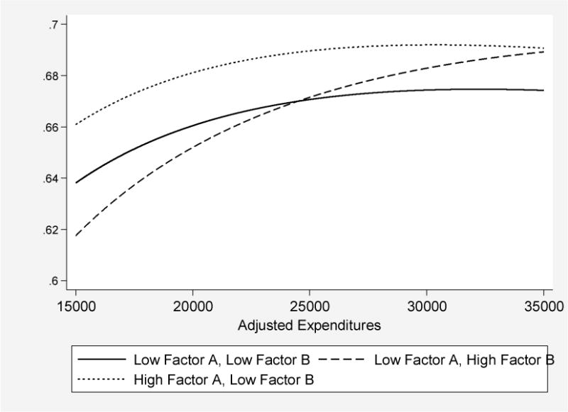
Note: The figure plots predicted one-year survival, based on regression analysis reported in Appendix Table A.2 with hospital fixed effects, for three hypothetical hospitals: A hospital that is one standard deviation below average on both adoption factors (Low Factor A, Low Factor B), a hospital that is one standard deviation below average on Factor B but one standard deviation above average on Factor A (High Factor A, Low Factor B), and a hospital that is one standard deviation below average on Factor A but one standard deviation above average on Factor B (Low Factor A, High Factor B). While the slope and shape of the production function comes directly off the estimated coefficients, the intercepts for each of these three curves are derived from a between-hospital regression of the hospital fixed effects regressed on the two factors, their squares, and their interactions.
Changes over time in diffusion rates
A prediction of the theoretical model is that hospitals which manage to improve their diffusion parameters will, like countries such as Japan or Korea in the postwar period, experience rapid growth in outcomes (Parente and Prescott, 2002), and conversely. Table 4 further considers risk-adjusted survival among hospitals which were initially in the slowest diffusion quintile (1) or the highest diffusion quintile (5) during 1994/95. For the slow-diffusion hospitals in 1994/95 remaining a slow diffusion hospital (in drug-eluting stents) in 2003/04, one-year survival rates rose from 65.2 percent in 1994/95 to 69.1 percent in 2003/04; an increase of 3.9 percent. Similarly, hospitals initially in the highest diffusing quintile (5) in 1993/94 which remained in the highest diffusing quintile by 2003/04, increased survival by 3.5 percentage points – very similar to the stable low-quintile hospitals, as predicted by the model.
Table 4.
Growth in Risk-Adjusted Survival by Diffusion Quintiles in 1994/95 and in 2003/04
| Survival: 1994/95 | Survival: 2003/04 | Change in Survival: 1994/95 to 2003/04 | ||||
|---|---|---|---|---|---|---|
| 2003/04 Quintile 1 (Slowest) |
2003/04 Quintile 5 (Fastest) |
2003/04 Quintile 1 (Slowest) |
2003/04 Quintile 5 (Fastest) |
2003/04 Quintile 1 (Slowest) |
2003/04 Quintile 5 (Fastest) |
|
| 1994/95 Quintile 1 (Slowest) |
0.652 (0.008) |
0.655 (0.019) |
0.691 (0.009) |
0.710 (0.012) |
0.039 (0.009) |
0.055 (0.016) |
| 1994/95 Quintile 5 (Fastest) |
0.686 (0.006) |
0.684 (0.005) |
0.701 (0.007) |
0.719 (0.006) |
0.015 (0.008) |
0.035 (0.006) |
Notes: The Table reports patient-weighted risk-adjusted 1-year survival rates in 1994–1995 and in 2003–2004, and the change in survival rates from 1994–1995 to 2003–2004. Each cell identifies hospitals according to whether they were in the fastest of slowest adoption quintile of effective treatments in 1994–1995 and whether they were in the fastest or slowest adoption quintile of drug-eluting stents in 2003–2004 (see Table 1). All standard errors are clustered at the hospital level.
Hospitals initially in the lowest diffusion quintile during 1994/95 but which moved up to the highest diffusion quintile for drug-eluting stents in 2003/04 (the “tigers”) experienced a gain of 5.5 percentage points. By contrast, the hospitals experiencing a decline in diffusion rates from quintile 5 in 1994/95 to quintile 1 in 2003/04 (the “turtles”) showed a survival gain of just 1.5 percentage points, significantly lower than the tigers (p = 0.03).14 These patterns are consistent with the view that changes in technology diffusion can be directly linked to changes in hospital outcomes as measured by patient survival.
6. Did the Rapid-Diffusion Hospitals Adopt Every New Innovation?
Thus far, we have considered only three of the many new innovations for heart attack patients during the period 1984–2004. Did the rapidly innovating hospitals also adopt other technologies across the board? Or does the adoption of these highly effective innovations reflect specific skills of the hospital management, as in the Lucas (1978) model of managerial skills? In this section, we consider three additional innovations with less cost-effective, and more heterogeneous benefits.
The first is lidocaine, a drug used to prevent ventricular fibrillation in AMI patients. While this was viewed as a promising approach in the early1980s, by the late 1980s a consensus had emerged that the use of lidocaine for uncomplicated AMIs could actually increase mortality (Hine, 1989); as of 1994/95, average rates of use were 20.4 percent.
The second is “late PCI”, or the use of angioplasty more than 12 hours after the index AMI. Beyond a small group of patients, its use was supported by either weak evidence or contraindicated (Ryan et al., 1993; pages 2048–49). Within a year of the AMI, 16.4 percent of all patients received such treatment. The third is coronary artery bypass surgery (CABG). The 1991 American College of Cardiology/American Heart Association (ACC/AHA) guidelines suggested strict criterion for CABG following AMI; and for many broad classes of patients, guidelines are not supportive.15 On average, 14.6 percent of AMI patients received CABG within a year of the AMI.
With these three additional technologies, we have a total of six diffusion measures created by averaging across all AMI patients in each hospital. We then estimated a factor model allowing for more than one factor using a varimax rotation, which facilitates interpretation of the factors by identifying each treatment rate with a single factor to the extent possible. The BIC goodness-of-fit criterion indicated just two distinct factors, labeled Factor A and Factor B. Note that we have not imposed any a priori restrictions on how these factors are estimated. As before, factor analysis normalizes the underlying factors to have a mean of zero and variance of one.
Factor A is nearly identical to our simple diffusion measure above; the correlation between the two is 0.98. To facilitate comparisons between Factor A and Factor B, we present in Table 5 the difference between Quintile 5 (fastest) and Quintile 1 (slowest) innovations, with the factor scoring weights (these weights are used to combine the six measures to form predictions of each factor). Factor A loads heavily on effective medical treatments that are highly effective such as aspirin (a weight of 0.41), beta blockers (0.35) and avoiding Lidocaine (−0.08). By contrast, Factor B loads more heavily on surgical innovations that tend to be less cost-effective such as reperfusion (0.27), PCI after 12 hours (0.20), CABG (0.15), as well as lidocaine (0.34). One interpretation of the two factors is that Factor A identifies hospitals that are able to accumulate new knowledge more quickly (and thereby more rapidly identify highly effective technologies), while Factor B identifies hospitals that are able to accumulate new technology more quickly (whether or not it is effective). Thus, Factor A seems to identify “smart” hospitals, while Factor B seems to identify “aggressive” hospitals.
Table 5.
Association of Factor A and B from 2-Factor Adoption Model with Adoption and Other Characteristics of the Hospital
| Factor A | Factor B | |||||
|---|---|---|---|---|---|---|
| Quintile 5 (Fastest) |
Quintile 1 (Slowest) |
Factor Scoring Weight | Quintile 5 (Fastest) |
Quintile 1 (Slowest) |
Factor Scoring Weight | |
| Aspirin | 0.90 | 0.65 | 0.41 | 0.82 | 0.75 | 0.07 |
| β Blocker | 0.65 | 0.31 | 0.35 | 0.41 | 0.51 | −0.15 |
| 12 Hour Reperfusion | 0.19 | 0.15 | 0.05 | 0.26 | 0.12 | 0.27 |
| Lidocaine | 0.17 | 0.21 | −0.08 | 0.32 | 0.11 | 0.34 |
| PCI after 12 hours | 0.22 | 0.12 | 0.13 | 0.23 | 0.10 | 0.20 |
| CABG | 0.18 | 0.12 | 0.10 | 0.18 | 0.10 | 0.15 |
| Average hospital volume* | 103 | 64 | 83 | 77 | ||
| Fraction major teaching hospital | 0.50 | 0.05 | 0.11 | 0.28 | ||
| Fraction for-profit hospital | 0.04 | 0.16 | 0.14 | 0.08 | ||
| Fraction government hospital | 0.10 | 0.17 | 0.14 | 0.13 | ||
| Average state income (1994/95, thousands) | 43.99 | 41.77 | 41.37 | 43.65 | ||
| Fraction of hospitals performing stents 2003 /04 | 0.82 | 0.28 | 0.75 | 0.31 | ||
| Of those, % Drug-Eluting Stent 2003/04 | 0.62 | 0.51 | 0.55 | 0.61 | ||
Volume for Medicare patients only.
Notes: Each column of the table reports average hospital and patient characteristics in the fastest and slowest adoption quintiles, and factor scoring weights for defining each factor, based on the factors estimated from a 2-factor model. The 2 factors were estimated from a factor model of hospital use of aspirin, β blockers reperfusion, Lidocaine, PCI after 12 hours (late PCI), and CABG (coronary artery bypass surgery). All averages are weighted by number of AMI patients in each hospital. All estimates except for stent data come from the Cooperative Cardiovascular Project (CCP), 1994–1995, with a sample of 139,847 AMI patients and 2999 hospitals. Estimates for each quintile are based on samples of approximately 28,000 AMI patients. Stent data are derived from Medicare Part A (hospital) claims from 2003–2004 for the same sample of hospitals.
There are other differences between the Factor A and B hospitals, also shown in Table 5, that are broadly consistent with this interpretation of the two factors. Unlike Factor A, there were no differences in patient volume across quintiles of Factor B, suggesting that the market may be rewarding “smart” adoption rather than the adoption of any new technology. Factor B hospitals also exhibit a higher fraction of for-profit hospitals (0.14 in the highest quintile versus 0.08 in the lowest) and a lower fraction of teaching hospitals (0.11 versus 0.28), suggesting that Factor B adoption is less related to knowledge of the medical staff. In sum, these two factors identify very different types of hospitals with very different strategies of technology adoption.
We first estimate the equivalent of Equation (13) with both factors, shown in Table 6; survival is a function of the continuous diffusion indices, log DRG inputs, and year fixed effects.16 As before, hospitals in the top quintile of Factor A are associated with 2.6 percentage point higher survival. By contrast, hospitals in the top Quintile for Factor B exhibit only 0.9 percentage point higher survival. Thus, adoption of the types of technologies associated with Factor B has less of an impact on survival than the highly effective technologies associated with Factor A.
Table 6.
Regression Estimates of Survival on DRG inputs and on Both Diffusion Factors from the 2-Factor model of Diffusion
| Dependent Variable | One-Year Survival | One-Year Survival |
|---|---|---|
| Factor A | 0.014 (0.001) |
|
| Factor A: Quintile 2 |
0.008 (0.002) |
|
| Factor A: Quintile 3 |
0.013 (0.002) |
|
| Factor A: Quintile 4 |
0.023 (0.002) |
|
| Factor A: Quintile 5 |
0.026 (0.002) |
|
| Factor B | 0.005 (0.001) |
|
| Factor B: Quintile 2 |
0.005 (0.002) |
|
| Factor B: Quintile 3 |
0.007 (0.002) |
|
| Factor B: Quintile 4 |
0.012 (0.003) |
|
| Factor B: Quintile 5 |
0.009 (0.003) |
|
| Log (DRG) | 0.020 (0.004) |
0.021 (0.004) |
| R2 | 0.09 | 0.09 |
Notes: Each column reports estimates from a separate regression in which an observation is a hospital-year, with N = 49,937 hospital-years. All regressions are weighted by the number of patients in each hospital-year. The dependent variable is the risk-adjusted one-year survival rate among AMI patients. The diffusion factors and quintiles are based on the 2-factor model described in Table 5. Log(DRG) is the log of the risk-adjusted total DRG weights per patient in the year following their AMI. Year dummy variables are included in all regressions. Risk-adjusted survival and DRG weights are derived from Medicare claims data from 1986–2004. The sample is limited to hospital/year observations with at least 5 observations per hospital. Standard errors (clustered at the hospital level) are in parentheses.
Finally, one might expect the return to factor inputs to be higher in hospitals that adopt technologies associated with Factor B, since these tend to be more expensive surgical interventions. We therefore estimate the more flexible “translog” production function (Christiansen, Jorgenson, and Lau, 1973) to allow for diminishing returns to πk, xit, and interaction between diffusion and the productivity of xit:
| (15) |
This allows, for example, a higher marginal return to the level of spending xit when hospitals invest more heavily in “B”-type innovations than “A”-type innovations.
The results of the fully interacted regression analysis are in Appendix Table A.2, with illustrative examples shown in Figure 3. We consider three types of hospitals. The first is one that eschews all types of technology adoption; it lies one standard deviation below the mean for both Factor A and Factor B, while the second is for hospitals like the first, except that the rate of diffusion for Factor A treatments is +1 standard deviation above the mean. As shown in Figure 3, the rapid Factor A adopting hospitals exhibit substantially better outcomes for their patients at all levels of spending, with marginal returns to additional inputs falling off rapidly above $25,000 per enrollee, roughly the mean value of spending in 2004.17 By contrast, the marginal returns to spending are strongly positive for hospitals with Factor B at +1 standard deviation above its mean. This is consistent with hospitals spending more if they are more rapid adopters of Factor B inputs, since the technologies typically entail billing more to Medicare. This is also consistent with Chandra and Staiger (2007), who find that hospitals specializing in surgical treatments can attain similar levels of outcomes to those specializing in medical treatments, albeit at higher costs, and with Doyle et al. (2010) who find that patients treated by physicians from a lower ranked medical school attain similar outcomes but require more resources to do so.
7. Conclusion
In this paper, we have attempted to peer inside the black box of hospital productivity changes both over time and across hospitals. We found that varying rates of adoption for low-cost but highly effective treatments explained a large fraction of the persistent differences in risk-adjusted survival during the period 1986–2004. Hospitals with the most rapid propensity to adopt these new innovations experienced survival rates nearly 3 percentage points above the lowest quintile hospitals, or nearly one-third the entire improvement in survival since 1986.
We also found distinct differences across hospitals with regard to which kinds of technologies were adopted. Some hospitals were far more likely to adopt beta blockers and aspirin, highly effective and inexpensive treatments, and these experienced consistently better survival outcomes than hospitals that invested more heavily in surgical treatments (such as PCI and CABG). While both types of hospitals experienced better overall outcomes than hospitals that failed to adopt any of the new technologies becoming available during the 1990s, hospitals that rapidly adopted beta blockers and aspirin had higher patient survival. Hall (2014) found similar results; regions adopting the cost-effective innovations like screening for colon cancer had better outcomes, while those with more rapid diffusion of low-effectiveness treatments, like breast cancer screening for women under age 50, did not.18 Our evidence suggests that knowledge about which technologies are most effective is a larger contributor to variation in productivity across hospitals than the adoption of new technology writ large.
Our model of health care productivity reconciles both the dramatic improvements in life expectancy for AMI patients over time (e.g., Cutler, 2004) and the mixed evidence on the efficiency of spending at a point in time (e.g., Fisher et al., 2003a,b; Doyle et al., 2014). Much of the dramatic growth in survival occurred as remarkably cost-effective treatments diffused across hospitals during the past few decades. For example, Ford et al. (2007) found aspirin and beta blockers to be among the most important factors reducing the number of AMI-related deaths between 1980–2000, followed by PCI and CABG. Of course, these estimates are specific to heart attacks, where the quality of clinical evidence is particularly good, and may not apply to other diseases where clinical guidelines are much weaker.
Chandra et al. (2013), using similar data on AMI patients, have developed an explicit model of productivity differences across hospitals (log survival minus log costs), and demonstrated that firms in non-health industries exhibit similar degrees of variation in productivity as do hospitals – in other words, that health care is not uniquely inefficient. Economists have identified a variety of optimizing economic models by which some firm adopt new innovations and others do not, which naturally lead to such productivity variations. For example, rational agents may adopt slowly because they are waiting for the price to decline (e.g., flat-screen TVs), or because of expertise in the older technology (Jovanovic and Nyarko, 1996). Alternatively, heterogeneity in production functions may lead to profit-maximizing differences in rates of diffusion (Griliches, 1957), or the presence of liquidity constraints may slow diffusion (Suri, 2011). Finally, there may be differences in education across workers (Nelson and Phelps, 1966) or technology complementary with skilled workers (Caselli and Coleman, 2006). While these theories may explain productivity differences in non-health sectors (and perhaps differences in adoption of new surgical innovations), they are less successful in explaining he slow diffusion of inexpensive beta blockers and aspirin by highly educated physicians.
Perhaps informational or organizational barriers explain the slow diffusion in both health and non-health sectors of the economy. Recall Equation (11), in which the marginal cost of speeding up diffusion C′(π), was set equal to the marginal benefit of innovating more rapidly. Using plausible parameters for measuring the social value of more rapid adoption suggests a very high equilibrium cognitive barrier facing physicians equal to $11,200 annually to move up one diffusion quintile.19 While this may appear to be implausibly high, previous research has shown that the quality of management, and in particular the presence of staff “opinion leaders,” can exert a disproportionate influence on individual physician adoption (Bradley, et al., 2001, 2005). This points to a more nuanced model of diffusion in which organizational support and “tactile” learning from peers (as in Keller, 2004), are critical for rapid diffusion. For this reason, we expect organizational inefficiencies, whether in non-health industries (Bloom and van Reenan, 2007) or in cardiac health centers for AMI patients (McConnell et al., 2013), are central to explaining why some hospitals were quick to adopt beta blockers and aspirin, and others were not.
Leibenstein (1966) used the term “X-efficiency” to describe residual differences in firm-level productivity which could not be readily explained by measured inputs or other factors. In many respects, the puzzle of slow diffusion for beta blockers and aspirin provides a textbook case of X-inefficiency. The underuse of aspirin and beta blockers was allowed to persist for so long because there was so little pressure exerted by markets or management to change old habits and adopt the new innovations. It is telling that the increased public hospital-level reporting of beta blocker use for AMI patients has been central to its nearly universal diffusion in the last decade, so much so that it is no longer used as a quality measure (Lee, 2007). More difficult is to explain why adoption behaviors are correlated between non-health sectors and health sectors, as in the close correlation across states in the adoption of hybrid corn in the 1930s and beta blockers in the 2000s (Skinner and Staiger, 2007).
There are several limitations to this study. First, our unit of analysis is the hospital, which by necessity aggregates up the adoption decisions of the physician. While some studies have used overlapping physician-hospital affiliations to identify hospital diffusion patterns (Sacarny, 2014), we are unable to determine which physician initiated specific treatments inside the hospital. Second, while we have direct evidence on why the rapidly-diffusing hospitals experienced better outcomes in 1994/95 from the CCP, we know much less about subsequent adoption patterns of the newer technologies such as the use of angiotensin receptor blockers (ARB) and angiotensin converting enzyme inhibitors (ACE inhibitors). Finally, our data is limited to Medicare enrollees age 65 and over, and there is little evidence on how (e.g.) beta blocker use in this population correlates with its use in the under-65 population.
Parente and Prescott (2002) provide a ready explanation for why some countries lag so far behind “frontier” countries: government restrictions and monopoly restraints that interfere with the benefits of efficient technology adoption. If patients both knew about the benefits of aspirin, beta blockers, and reperfusion, and were sensitive to published and reliable information about hospital quality, physicians would be forced to respond rapidly to new innovations or face the loss of patients. But when quality measures are limited, patients are not well informed, and markets are distorted, remarkably large inefficiencies can persist across hospitals and over time.
Figure 2.

Interpreting the Evidence on Survival and Health Outcomes: “Flat of the Curve” vs. Productivity Differentials
Acknowledgments
We are grateful to seminar participants, and to Mary Burke, David Card, Amitabh Chandra, James Feyrer, Elliott Fisher, Sherry Glied, Anne Hall, Caroline Hoxby, Peter Klenow, Justin McCrary, David Weil, Milton Weinstein, Jack Wennberg, and an anonymous referee for helpful comments. Weiping Zhou and Daniel Gottlieb provided excellent data analysis. We are indebted to the National Institute on Aging (PO1- AG19783 and U01 – AG046830) and to the Robert Wood Johnson Foundation for financial support.
Appendix: The Derivation of the Dynamic Model
We rewrite the objective function (7) for hospital i at time t as Equation A.1:
| (A.1) |
The basic model – in which saving lives is good, and spending more is bad – is consistent with a range of models trying to capture what it is that hospitals maximize. For example, consider a model in which there exists a tension between two goals of the hospital: to maximize social welfare – the value of lives saved less resource costs – and the desire to maintain financial stability by maximizing profits. Suppose that the relative weight between the two objectives is given by μi, which is hospital-specific and ranges between one (the hospital maximizes social welfare without regard to its own financial position) and zero (the hospital cares solely about maximizing profit). Thus the objective function is
| (A.2) |
in which Ψ* is the true social value of survival, ωi the marginal proportional contribution to profitability of an incremental Xit, and Kit, the fixed subsidization or fixed costs, and Pit the factor cost, are defined as above. It is straightforward to show that (A.1) is a “reduced-form” version of (A.2), where Ψi = μi Ψ* and φi = μi−ωi(1−μi). Note that φi>0 for the solution to exist (since the marginal productivity of Xit in this log-linear production function never turns negative), so the temptation to provide a highly profitable procedure must be tempered by at least some desire to curb allocative inefficiency.
The discrete discrete-time Lagrangian based on A.1 is written
| (A.3) |
The first-order conditions are written:
| (A.4a) |
| (A.4b) |
| (A.4c) |
| (A.4d) |
In addition to these four first-order conditions, we also add a solvency constraint:
| (A.4e) |
to ensure the present value of profits is non-negative (although hospitals can lose money in a given year). While hospitals do go out of business, we seek to avoid these more complicated issues by focusing solely on hospitals that remain in the panel during the period of analysis.
We first characterize the equilibrium, and demonstrate that a steady-state solution exists: πit = πi. To show this, we first solve for λit. Dropping the i subscript and assuming a constant π, (A.3c) is written
| (A.5) |
and by progressive substitution:
| (A.6) |
Solving for the infinite series (which converges given that π and r > 0) and assuming that the transversality condition is met, so that λk(1−π)k converges to zero as k gets large, λ0=Ψ/(π + r). From A.5,
By successive substitution, λt = λt−1/(1 + r). This in turn implies a steady-state solution for Xit = Xi (since both λ and the objective function decay at the rate r).
By rearranging A.4b and substituting for λt, one can derive Equation (11) in the text. By further substituting (1−π)/π for (at* − at), which comes from the steady-state expression in Equation (10), we can also write the solution for π as:
| (A.7) |
Simulations of this key first-order condition suggests a high degree of dynamic stability.
Differential Rates of Diffusion Across Innovations
Suppose there were two general classes of innovations, A and B, each of which contributes to total hospital factor productivity: ait=αAit+αBit. Every year there are two new technologies that become available, one in Class A and one in Class B, with incremental value αA and αB, respectively. Thus Equation (3) can be generalized to:
| (A.8) |
With two separate diffusion parameters πAi and πBi for each hospital i. If we assume that the cost of diffusion differs for the two classes, then the steady state diffusion parameters will differ for technologies in Class A and B.
We can therefore approximate the adoption of each technology at any point in time, given by mkjit=1−(1−πki)t−j (k = A, B), by taking a first-order Taylor-series approximation:
| (A.9) |
The structure in Equation (13) is consistent with a factor model across the j different technologies that depend on two underlying factors, πAi and πBi, with loading factors equal to (t-j), and where vkjit is a stochastic element that allows for random fluctuations over time. This in turn allows us to rewrite (12) as a linear approximation of each diffusion parameter and inputs x:
| (A.10) |
Appendix Table A.1.
Basic Risk Adjustment Model
| One-Year Survival | One-Year Expenditures | ||
|---|---|---|---|
| Mean | Coefficient | Coefficient | |
| Vascular Disease | 0.070 | −0.028 (0.001) |
1658 (55) |
| Pulmonary Conditions | 0.187 | −0.081 (0.001) |
1368 (37) |
| Dementia | 0.026 | −0.135 (0.002) |
−4919 (84) |
| Diabetes | 0.246 | −0.039 (0.001) |
1948 (33) |
| Liver Disease | 0.003 | −0.240 (0.005) |
−2019 (269) |
| Renal Disease | 0.024 | −0.278 (0.002) |
1256 (94) |
| Cancer | 0.042 | −0.164 (0.001) |
−2716 (70) |
| Location of MI | |||
| Anterolateral | 0.042 | −0.003 (0.002) |
685 (122) |
| Anterior Wall | 0.165 | 0.033 (0.002) |
1117 (107) |
| Inferolateral | 0.029 | 0.062 (0.002) |
331 (130) |
| Inferior Posterior | 0.021 | 0.073 (0.002) |
1033 (140) |
| Inferior Wall | 0.178 | 0.102 (0.002) |
333 (106) |
| Lateral (NEC) | 0.021 | 0.066 (0.003) |
−114 (139) |
| True Posterior | 0.007 | 0.073 (0.004) |
825 (194) |
| Sub-Endocardial | 0.414 | 0.119 (0.002) |
2092 (103) |
| AMI (NEC) | 0.022 | — | — |
| AMI (NOS) | 0.100 | −0.093 (0.002) |
−1783 (111) |
| Constant (for non-black male age 65–69 | 0.733 (0.004) |
24308 (166) |
|
| Age-Sex-Race-Year Categorical Variables | Yes | Yes | |
| Sample Size | 3,185,837 | 2,808,171 | 2,808,170 |
Note. Standard error of estimate in parentheses. Coefficients are from a patient-level regression of survival or expenditures that also included hospital-year fixed effects, using Medicare claims data from 1986–2004.
Appendix A.2.
Coefficients of Translog Production Function Estimate with Factor A and Factor B
| Without Hospital Fixed Effects | With Hospital Fixed Effects | |
|---|---|---|
| ln(DRG) | 0.319 (0.018) |
0.227 (0.017) |
| ln(DRG)2 | −0.106 (0.007) |
−0.063 (0.006) |
| Factor A | 0.028 (0.004) |
|
| Factor A2 | 0.0003 (0.008) |
|
| Factor A * ln(DRG) | −0.010 (0.002) |
−0.004 (1.46) |
| Factor B | −0.021 (0.005) |
|
| Factor B2 | −0.004 (0.001) |
|
| Factor B * ln(DRG) | 0.017 (0.004) |
0.021 (0.003) |
| Factor A * Factor B | 0.004 (0.002) |
|
| R2 | 0.10 | 0.27 |
Notes: Each column presents regression results from a generalized translog production function (year effects included but not reported), clustered at the hospital level. The dependent variable is one-year risk-adjusted survival. Column 1 presents coefficients without hospital-level fixed effects; Column 2 includes hospital-level fixed effects. Note that many of the Factor A and Factor B coefficients drop out of Column 2 because of hospital fixed effects. For sample description and variable definitions see the notes to table 6.
Footnotes
See e.g., Fuchs (2004) and Enthoven (1978).
In his 1601 voyage to India, Captain James Lancaster fed sailors in one of his ships 3 teaspoons of lemon juice every day, while in the other three ships, no lemon juice was provided. By the midpoint of the journey, 110 of the 278 sailors in the control group had died of scurvy (40 percent), while none of the sailors in the treatment group had been affected (Berwick, 2003).
Strictly speaking, neither aspirin nor beta blockers were “innovations” as they had been in use for decades; the innovation was to use these drugs in treating AMI patients.
The distinction between medical and surgical treatments for AMI follows Chandra and Staiger (2007).
In theory one could measure physical inputs as hospital days and physician resource-value units (RVUs), but neither captures treatment intensity. See Jacobs, Smith, and Street (2006) for an excellent discussion of productivity in the quantity of medical services, X.
This model can also be written in continuous time as a current-value Hamiltonian, but we maintain a discrete time structure to be consistent with the empirical data.
Optimal factor inputs are independent of the level of technology because the production function (Equation 2) assumes that the marginal product of factor inputs (β) does not depend on technology. In a more general specification that allowed for interactions between technology and factor inputs, optimal factor inputs would increase (decrease) if new technology increased (decreased) the marginal product of factor inputs.
Hospitals included in this sample were required to have remained in existence throughout the period 1986–2004 in the Medicare claims data, as described in Section 6.
These averages are for all patients and not for “ideal” patients; since it is often difficult in practice to define ideal or appropriate patients. While a high fraction of patients should receive β blockers and aspirin, the optimal rate for revascularization is substantially lower.
The estimated effect of beta blockers is a 22 percent decline in one-year mortality arising from beta blockers (Phillips, et al., 2000), times a baseline 33 percent mortality probability. For aspirin, mortality was 18 percent lower (Krumholz et al. 1995). For 12-hour reperfusion, we use as a lower bound the impact of fibrinolytic therapy, of about 25 percent mortality decline (FTT, 1994). Each of these were multiplied by the gap across quintiles (from Table 1) in the corresponding diffusion measures.
While there has been some controversy about the health benefits of drug-eluting stents (see Malenka, et al., 2008), there was widespread consensus among cardiologists in 2003 that this new technology was better than the older bare-metal stents. Also note that the estimated diffusion rates are for all stenting patients, and not solely AMI patients.
For example, an AMI patient fitted with a drug-eluting stent would qualify for 3.12 DRG “units” in 2003, and this was common across all hospitals. Note that DRG weights may change slightly over time.
If aspirin began diffusing in 1975, beta blockers in 1985, and reperfusion in 1992 (all reasonable start dates), then by 1995 diffusion rates of 10% and 5% would generate aspirin use of 88% and 64%, beta blocker use of 65% and 40%, and reperfusion use of 27% and 14%, which are reasonably consistent with estimates in Table 1.
One hypothesis is that hospitals that were early adopters of surgery in 1994/95 would also be early adopters of drug-eluting stents in 2003/04, and so the improved survival of the “tiger” hospitals was simply the consequence of surgical innovations paying off in the 2000s. However, drug-eluting stents were no more correlated with surgical procedure rates in 1994/95 than beta blockers or aspirin in 1994/95.
For example: “The coronary artery bypass operation probably has little place in the management of most patients with uncomplicated acute Q wave myocardial infarction, but the matter remains arguable.” (Kirklin et al., 1991, page 1141.)
We show in the Appendix that a model in which there are two types of innovations that appear in each year, a higher-value and lower-value innovation, leads to an estimation equation that is identical to Equation (13), except to include both of the diffusion parameter for Factor A, πAi, and Factor B, πBi.
To facilitate the interpretation of the regression, we multiplied the DRG inputs times a constant, the national average reimbursement per DRG in 2004, leading to a dollar amount that corresponds to the DRG inputs.
She also found that high-adoption hospitals tended to adopt all new technologies (Hall, 2014). This may appear to be inconsistent with our model, but when we use a principal components approach (as she does), we find similar results. In principal component models, the first component splits out regions that adopt anything (either Factor A or Factor B) versus those that do not.
We assume that the average lag from the frontier, at* − at = 0.02, Ψ = $100,000, the one-year survival following AMI translates to an additional 5.25 life-years, r = .05, πA must increase by 0.016 to shift to the next quintile, and there are 10 AMI patients per physician.
Contributor Information
Jonathan Skinner, Email: jonathan.skinner@dartmouth.edu, Dartmouth and NBER.
Douglas Staiger, Email: douglas.staiger@dartmouth.edu, Dartmouth and NBER.
References
- Baicker Katherine, Chandra Amitabh. Medicare Spending, The Physician Workforce, and The Quality of Health Care Received by Medicare Beneficiaries. Health Affairs. 2004:184–97. doi: 10.1377/hlthaff.w4.184. [DOI] [PubMed] [Google Scholar]
- Berndt Ernst R, Bir Anupa, Busch Susan H, Frank Richard G, Normand Sharon-Lise T. The Medical Treatment of Depression, 1991–1996: Productive Inefficiency, Expected Outcome Variations and Price Indexes. Journal of Health Economics. 2002;21:373–396. doi: 10.1016/s0167-6296(01)00132-1. [DOI] [PubMed] [Google Scholar]
- Bero Lisa A, Grilli Roberto, Grimshaw Jeremy M, et al. Closing the Gap Between Research and Practice: An Overview of Systematic Reviews of Interventions to Promote the Implementation of Research Findings. British Medical Journal. 1998;317:465–468. doi: 10.1136/bmj.317.7156.465. [DOI] [PMC free article] [PubMed] [Google Scholar]
- Berwick Donald M. Disseminating Innovations in Health Care. JAMA. 2003;289:1969–1975. doi: 10.1001/jama.289.15.1969. [DOI] [PubMed] [Google Scholar]
- Bloom Nicholas, Van Reenen John. Measuring and Explaining Management Practices Across Firms and Countries. Quarterly Journal of Economics. 2007;122:1351–1408. [Google Scholar]
- Bradley Elizabeth H, Holmboe Eric S, Mattera Jennifer A, et al. A Qualitative Study of Increasing β-Blocker Use After Myocardial Infarction: Why Do Some Hospitals Succeed? JAMA. 2001;285:2604–2611. doi: 10.1001/jama.285.20.2604. [DOI] [PubMed] [Google Scholar]
- Bradley Elizabeth H, Herrin Jeph, Mattera Jennifer A, Holmboe Eric S, Wang Yongfei, et al. Quality Improvement Efforts and Hospital Performance: Rates of Beta-Blocker Prescription After Acute Myocardial Infarction. Medical Care. 2005;43:282–92. doi: 10.1097/00005650-200503000-00011. [DOI] [PubMed] [Google Scholar]
- Caselli Francesco, Coleman Wilbur John., II The World Technology Frontier. American Economic Review. 2006;96:499–522. [Google Scholar]
- Chandra Amitabh, Staiger Douglas. Testing a Roy Model with Productivity Spillovers: Evidence from the Treatment of Heart Attacks. Journal of Political Economy February. 2007 doi: 10.1086/512249. [DOI] [PMC free article] [PubMed] [Google Scholar]
- Chandra Amitabh, Finkelstein Amy, Sacarny Adam, Syverson Chad. (NBER Working Paper 19200).Healthcare Exceptionalism? Productivity and Allocation in the US Healthcare Sector. 2013 [Google Scholar]
- Chandra Amitabh, Skinner Jonathan. Technology Growth and Expenditure Growth in Health Care. Journal of Economic Literature. 2012;50:645–80. [Google Scholar]
- Comin Diego, Hobijn Bart. An Exploration of Technology Diffusion. American Economic Review. 2010;100:2031–59. [Google Scholar]
- Comin Diego A, Mestieri Marti. (NBER Working Paper 19052).Technology Diffusion: Measurement, Causes and Consequences. 2013 [Google Scholar]
- Christensen Laurits R, Jorgenson Dale W, Lau Lawrence J. Transcendental Logarithmic Production Frontiers. The Review of Economics and Statistics. 1973;55:28–45. [Google Scholar]
- Crespi Gustavo, Criscuolo Chiara, Haskel Jonathan E, Slaughter Matthew. (NBER Working Paper 13959).Productivity Growth, Knowledge Flows, and Spillovers. 2008 http://www.nber.org/papers/w13959.
- Cutler David M, McClellan Mark, Newhouse Joseph P, Remler Dahlia. Are Medical Prices Declining? Evidence from Heart Attack Treatments. Quarterly Journal of Economics. 1998;93:991–1024. [Google Scholar]
- Cutler David M. Your Money or Your Life: Strong Medicine for America’s Health Care System. New York: Oxford University Press; 2004. [Google Scholar]
- Cutler David M, Skinner Jonathan, Stern Ariel Dora, Wennberg David. (NBER Working Paper No. 19320).Physician Beliefs and Patient Preferences: A New Look at Regional Variation in Health Care Spending. 2013 doi: 10.1257/pol.20150421. [DOI] [PMC free article] [PubMed] [Google Scholar]
- Doyle Joseph J., Jr Returns to Local-Area Healthcare Spending: Evidence from Health Shocks to Patients Far From Home. American Economic Journals: Applied Economics. 2011;3:221–243. doi: 10.1257/app.3.3.221. [DOI] [PMC free article] [PubMed] [Google Scholar]
- Doyle Joseph J, Jr, Ewer Steven M, Wagner Todd H. Returns to Physician Human Capital: Evidence from Patients Randomized to physician teams. Journal of Health Economics. 2010;29:866–882. doi: 10.1016/j.jhealeco.2010.08.004. [DOI] [PubMed] [Google Scholar]
- Doyle Joseph J, Jr, Graves John A, Gruber Jonathan, Kleiner Samuel. Do High-Cost Hospitals Deliver Better Care? Evidence from Ambulance Referral Patterns. Journal of Political Economy. 2014 doi: 10.1086/677756. forthcoming. [DOI] [PMC free article] [PubMed] [Google Scholar]
- Eaton Jonathan, Kortum Samuel. International Technology Diffusion: Theory and Measurement. International Economic Review. 1999;40:537–570. [Google Scholar]
- Enthoven Alan C. Shattuck Lecture—Cutting Cost without Cutting the Quality of Care. New England Journal of Medicine. 1978;298:1229–1238. doi: 10.1056/NEJM197806012982204. [DOI] [PubMed] [Google Scholar]
- Fisher Elliott S, Wennberg David, Stukel Therese, Gottlieb Daniel, Lucas FL, Pinder Etoile L. The Implications of Regional Variations in Medicare Spending. Part 2: Health Outcomes and Satisfaction With Care. Annals of Internal Medicine. 2003;138:288–299. doi: 10.7326/0003-4819-138-4-200302180-00007. [DOI] [PubMed] [Google Scholar]
- FTT (Fibrinolytic Therapy Trialists’ Collaborative Group) Indications for Fibrinolytic Therapy in Suspected Acute Myocardial Infarction: Collaborative Overview of Early Mortality and Major Morbidity Results from All Randomised Trials of More than 1000 Patients. Fibrinolytic Therapy Trialists’ (FTT) Collaborative Group. Lancet. 1994;343:311. [PubMed] [Google Scholar]
- Ford Earl S, Ajini Umed A, Croft Janet B, et al. Explaining the Decrease in U.S. Deaths from Coronary Disease, 1980–2000. NEJM. 2007;356:2388–2398. doi: 10.1056/NEJMsa053935. [DOI] [PubMed] [Google Scholar]
- Fuchs Victor R. More Variation In Use Of Care, More Flat-Of-The-Curve Medicine. Health Affairs. 2004 doi: 10.1377/hlthaff.var.104. Web Exclusive. [DOI] [PubMed] [Google Scholar]
- Griliches Zvi. Hybrid Corn: An Exploration in the Economics of Technological Change. Econometrica. 1957;25:501–522. [Google Scholar]
- Hall Anne. Regional Medical Technology Adoption Patterns, Their Effects on Health Care Productivity, and Their Determinants. Working Paper Bureau of Economic Analysis. 2014 [Google Scholar]
- Hall Bronwyn. Innovation and Diffusion. In: Jan Fagerberg, Mowery David C, Nelson Richard R., editors. Handbook on Innovation. Oxford: Oxford University Press; 2004. [Google Scholar]
- Hall Robert E, Jones Charles I. Why Do Some Countries Produce So Much More Output Per Worker Than Others? Quarterly Journal of Economics. 1999;114:83–116. [Google Scholar]
- Hirth Richard A, Chernew Michael E, Miller Edward, Fendrick A Mark, Weissert William G. Willingness to Pay for a Quality-Adjusted Life Year: In Search of a Standard. Medical Decision Making. 2000;20:332–342. doi: 10.1177/0272989X0002000310. [DOI] [PubMed] [Google Scholar]
- Hine Louis K, Laird Nan, Hewitt Peg, Chalmers Thomas C. Meta-analytic Evidence Against Prophylactic Use of Lidocaine in Acute Myocardial Infarction. Archives of Internal Medicine. 1989;149:2694–2698. [PubMed] [Google Scholar]
- Horwitz Jill, Nichols Austin. (NBER Working Paper 13246).What do Nonprofits Maximize? Nonprofit Hospital Service Provision and Market Ownership Mix. 2007 [Google Scholar]
- ISIS-2: The Second International Study of Infarct Survival Collaborative Group. Randomised Trial of Intravenous Streptokinase, Oral Aspirin, Both, or Neither among 17,187 Cases of Suspected Acute Myocardial Infarction: ISIS-2. Lancet. 1988;32:349–360. [PubMed] [Google Scholar]
- Jacobs Rowena, Smith Peter C, Street Andrew. Measuring Efficiency in Health Care: Analytic Techniques and Health Policy. New York: Cambridge University Press; 2006. [Google Scholar]
- Jencks Stephen F, Huff Edwin D, Cuerdon Timothy. Change in the Quality of Care Delivered to Medicare Beneficiaries, 1998–99 to 2000–2001. JAMA. 2003;289:305–312. doi: 10.1001/jama.289.3.305. [DOI] [PubMed] [Google Scholar]
- Jovanovic Boyan, Nyarko Yaw. Learning by Doing and the Choice of Technology. Econometrica. 1996;64:1299–1310. [Google Scholar]
- Keller Wolfgang. International Technology Diffusion. Journal of Economic Literature. 2004;42:752–82. [Google Scholar]
- King Joseph T, Jr, Tsevat Joel, Lave Judith R, Roberts Mark S. Willingness to Pay for a Quality-Adjusted Life Year: Implications for Societal Health Care Resource Allocation. Medical Decision Making. 2005;25:667–677. doi: 10.1177/0272989X05282640. [DOI] [PubMed] [Google Scholar]
- Kirklin John W, Akins Cary W, Blackstone Eugene H, Booth David C, Califf Robert M, et al. ACC/AHA Guidelines and Indications for Coronary Artery Bypass Graft Surgery: A Report of the American College of Cardiology/American Heart Association Task Force on Assessment of Diagnostic and Therapeutic Cardiovascular Procedures. Circulation. 1991;83:1125–1173. doi: 10.1161/01.cir.83.3.1125. [DOI] [PubMed] [Google Scholar]
- Krumholz Harlan M, Radford Martha J, Ellerbeck Edward F, Hennen John, Meehan Thomas P, et al. Aspirin in the treatment of acute myocardial infarction in elderly Medicare beneficiaries. Patterns of use and outcomes. Circulation. 1995;92:2841–7. doi: 10.1161/01.cir.92.10.2841. [DOI] [PubMed] [Google Scholar]
- Lee Thomas H. Eulogy for a Quality Measure. New England Journal of Medicine. 2007;357:1175–77. doi: 10.1056/NEJMp078102. [DOI] [PubMed] [Google Scholar]
- Leibenstein Harvey. Allocative Efficiency vs. ‘X-efficiency. American Economic Review. 1966;56:392–415. [Google Scholar]
- Lucas Robert E. On the Size Distribution of Business Firms. The Bell Journal of Economics. 1978;9:508–23. [Google Scholar]
- Malenka David J, Kaplan Aaron V, Lucas Lee, Sharp Sandra M, Skinner Jonathan S. Outcomes Following Coronary Stenting in the Era of Bare Metal versus the Era of Drug Eluting Stents. JAMA. 2008;299:2868–2876. doi: 10.1001/jama.299.24.2868. [DOI] [PMC free article] [PubMed] [Google Scholar]
- McConnell K John, Lindrooth Richard C, Wholey Douglas R, Maddox Thomas M, Bloom Nick. Management Practices and the Quality of Care in Cardiac Units. JAMA Internal Medicine. 2013;173:684–692. doi: 10.1001/jamainternmed.2013.3577. [DOI] [PubMed] [Google Scholar]
- Murphy Kevin M, Topel Robert H. The Value of Health and Longevity. Journal of Political Economy. 2006;114:871–904. [Google Scholar]
- Nelson Richard R, Phelps Edmund S. Investment in Humans, Technological Diffusion, and Economic Growth. American Economic Review. 1966;56:69–75. [Google Scholar]
- Parente Stephen L, Prescott Edward C. Barriers to Technology Adoption and Development. The Journal of Political Economy. 1994;102:298–321. [Google Scholar]
- Parente Stephen L, Prescott Edward C. Barriers to Riches. Cambridge: MIT University Press; 2002. [Google Scholar]
- Phelps Charles E. Information Diffusion and Best Practice Adoption. In: Culyer AJ, Newhouse JP, editors. Handbook of Health Economics. Vol. 1. Elsevier Science; 2000. [Google Scholar]
- Phillips Kathryn A, Shlipak Micheal G, Coxson Pam, et al. Health and Economic Benefits of Increased β Blocker Use Following Myocardial Infarction. JAMA. 2000;284:2748–2754. doi: 10.1001/jama.284.21.2748. [DOI] [PubMed] [Google Scholar]
- Rogers EM. Diffusion of Innovations. 5. New York: The Free Press; 2003. [Google Scholar]
- Ryan Thomas J, Bauman William B, Kennedy J Ward, Kerelakes Dean J, King Spencer B, McCallister Ben D, Smith Sidney C, Ullyot Daniel J. Guidelines for Percutaneous Transluminal Coronary Angioplasty. Journal of the American College of Cardiology. 1993;22:2033–54. [Google Scholar]
- Sacarny Adam. (Working Paper Harvard University).Technological Diffusion Across Hospitals: The Case of a Revenue-Generating Practice. 2014 [Google Scholar]
- Skinner Jonathan, Fisher Elliott, Wennberg John E. The Efficiency of Medicare. In: Wise D, editor. Analyses in the Economics of Aging. University of Chicago Press and NBER; 2005. pp. 129–57. [Google Scholar]
- Skinner Jonathan, Staiger Douglas. Technological Diffusion from Hybrid Corn to Beta Blockers. In: Berndt E, Hulten CM, editors. Hard-to-Measure Goods and Services: Essays in Honor of Zvi Griliches. University of Chicago Press and NBER; 2007. [Google Scholar]
- Suri Tavneet. Selection and Comparative Advantage in Technology Adoption. Econometrica. 2011;79:159–209. [Google Scholar]
- Yusuf S, Peto R, Lewis J, Collins R, Sleight P. Beta blockade during and after myocardial infarction: an overview of the randomized trials. Progress in Cardiovascular Diseases. 1985;27:335–71. doi: 10.1016/s0033-0620(85)80003-7. [DOI] [PubMed] [Google Scholar]