

Abstract
Motivation: The de novo identification of the initiation and termination zones—regions that replicate earlier or later than their upstream and downstream neighbours, respectively—remains a key challenge in DNA replication.
Results: Building on advances in deep learning, we developed a novel hybrid architecture combining a pre-trained, deep neural network and a hidden Markov model (DNN-HMM) for the de novo identification of replication domains using replication timing profiles. Our results demonstrate that DNN-HMM can significantly outperform strong, discriminatively trained Gaussian mixture model–HMM (GMM-HMM) systems and other six reported methods that can be applied to this challenge. We applied our trained DNN-HMM to identify distinct replication domain types, namely the early replication domain (ERD), the down transition zone (DTZ), the late replication domain (LRD) and the up transition zone (UTZ), using newly replicated DNA sequencing (Repli-Seq) data across 15 human cells. A subsequent integrative analysis revealed that these replication domains harbour unique genomic and epigenetic patterns, transcriptional activity and higher-order chromosomal structure. Our findings support the ‘replication-domain’ model, which states (1) that ERDs and LRDs, connected by UTZs and DTZs, are spatially compartmentalized structural and functional units of higher-order chromosomal structure, (2) that the adjacent DTZ-UTZ pairs form chromatin loops and (3) that intra-interactions within ERDs and LRDs tend to be short-range and long-range, respectively. Our model reveals an important chromatin organizational principle of the human genome and represents a critical step towards understanding the mechanisms regulating replication timing.
Availability and implementation: Our DNN-HMM method and three additional algorithms can be freely accessed at https://github.com/wenjiegroup/DNN-HMM. The replication domain regions identified in this study are available in GEO under the accession ID GSE53984.
Contact: shuwj@bmi.ac.cn or boxc@bmi.ac.cn
Supplementary information: Supplementary data are available at Bioinformatics online.
1 Introduction
Complete and accurate chromosomal DNA replication is crucial for proper cell division and maintenance of the genetic integrity in all organisms (Bell and Dutta, 2002). In eukaryotes, DNA replication begins and ends at multiple genomic regions, designated the replication initiation and termination zones, respectively, according to a tightly controlled spatiotemporal order (Masai et al., 2010; Sclafani and Holzen, 2007). Dysregulation of initiation or termination may delay genomic replication, resulting in various diseases (Bicknell et al., 2011a, b; Guernsey et al., 2011; Letessier et al., 2011) and even cancer (Suzuki and Takahashi, 2013; Woo and Li, 2012).
The initiation and termination zones may be identified from the replication timing profiles as regions that replicate earlier or later, respectively, than their upstream and downstream neighbours (Schwaiger et al., 2009). The timing of the replication of a given DNA sequence is determined by its distance from the local active replication origin and by the timing of the firing of that origin during the S phase (Schwaiger et al., 2009). Genome-wide replication timing profiles have been used to identify replication origins throughout Saccharomyces cerevisiae (Raghuraman et al., 2001) and in higher eukaryotes, including Drosophila (MacAlpine et al., 2004; Schubeler et al., 2002; Schwaiger et al., 2009), mice (Farkash-Amar et al., 2008) and human (Audit et al., 2007; Karnani et al., 2007; Lucas et al., 2007; Woodfine et al., 2005). These studies revealed that the timing of DNA replication is associated with transcriptional activity, epigenetic patterns and higher-order nuclear structures. However, the genomic, epigenetic and transcriptional signatures that define the early late replication domain (ERDs) and late replication domain (LRD) in the human genome have not been fully elucidated. In particular, the strengths of the correlations between replication timing and the chromatin status within ERD and LRD across diverse human cell types remain unclear. Furthermore, the molecular mechanisms through which the chromatin patterns are established and maintained within the ERD and LRD in the human genome remain poorly understood. Resolving these questions completely depends on the precise identification of the ERD and LRD in the human genome, which remains one of the greatest challenges in bioinformatics research. To date, very few bioinformatics methods have been proposed for the de novo identification of replication domains using replication timing profiles.
Recently, deep learning approaches have surpassed the state- of-the-art performance of previous methods for many tasks (Bengio et al., 2013), due to their powerful capacity to automatically learn features at multiple levels of abstraction directly from data without using human-crafted features or rules (Bengio, 2009). The Deep Neural Network (DNN) was developed from the Artificial Neural Network (ANN) with the advent of the deep learning algorithm (Bengio, 2009; Bengio et al., 2013). Compared with a shallow-learning model that included an ANN and Gaussian mixture model (GMM), the deep learning model, i.e. DNN, consists of multiple hidden layers showing significantly greater power to representation data than the shallow model and is widely applied in computer vision, dimensionality reduction and speech recognition. In addition, hidden Markov models (HMMs) are well known for their effectiveness in the modelling of sequential patterns of data and have been extensively applied in computational biology, specifically in biological sequence analysis, Copy Number Variation detection, motif finding, breakpoints identification and chromatin state discovery. These advances triggered our interest in developing a novel hybrid architecture between a pre-trained DNN and an HMM for the de novo identification of replication domains using replication timing profiles.
In this study, we present the first DNN–HMM hybrid model, which combines the representational power of DNNs and the sequential modelling capacity of HMMs to successfully resolve the challenge of the de novo identification of replication domains using newly replicated DNA sequencing (Repli-Seq) data. We demonstrate that DNN–HMMs can significantly outperform strong discriminatively trained GMM–HMM systems and other six reported methods that can be applied to this challenge. We applied our trained DNN–HMM to the identification of distinct types of replication domains, including the ERD, the down transition zone (DTZ), the LRD, and the up transition zone (UTZ), using Repli-Seq data across 15 human cell types. A subsequent integrative analysis based on ENCODE data revealed that the replication domains of distinct types harbour unique genomic and epigenetic patterns, transcriptional activity and higher-order chromosomal structure. Our findings support the ‘replication-domain’ model, which states that ERDs and LRDs, connected by UTZs and DTZs, are spatially compartmentalized structural and functional units of higher-order chromosomal structure. In our model, the adjacent DTZ-UTZ pairs form a chromatin loop, and intra-interactions within ERDs and LRDs tend to be short- and long-range, respectively. Our model reveals an important chromatin organizational principle of the human genome and represents a critical step towards increasing our understanding of the mechanisms regulating replication timing.
2 Materials and methods
2.1 Deep belief networks
In contrast to the discriminative nature of traditional neutral nets, deep belief networks (DBNs), initially introduced by Hinton et al. (2006), are probabilistic generative models. DBNs consist of several layers of Restricted Boltzmann Machines (RBMs) (Hinton, 2009), which are a type of undirected bipartite graph constructed from a bottom layer of binary stochastic hidden units and a top layer of stochastic visible units . For an RBM, an energy function is assigned to the configurations of and , and this function is of the following form
| (1) |
where is the symmetrical matrix of visible/hidden connection weights and and are the biases of the visible and hidden units, respectively. Thus, the probability distribution of any particular setting of and is
| (2) |
where the normalization factor is known as the partition function. The bipartite and binary natures of RBMs enable us to derive simple exact expressions for and as
| (3) |
and
| (4) |
respectively, where denotes the (elementwise) logistic sigmoid and equals .
In our algorithm, RBMs were trained in a greedy layer-wise manner with one-step contrastive divergence (CD-1). We used the DBN weights resulting from RBMs to initialize DNNs generatively in a purely unsupervised way and used the outputs of DBN as the inputs to train the Softmax output layer in a supervised manner. After pre-training, we used a backpropagation algorithm to fine-tune all of the weights in a supervised manner to improve the discriminative performance of the entire network. Pre-training followed by stochastic gradient descent is used to train DNN because it often outperforms random initialization for the deeper architectures and provides robust results to the initial random seed. Studies have illustrated that using DBN pre-training to initialize the weights of a DNN helps prevent overfitting and can aid in subsequent optimization and can reduce generalization error (Erhan et al., 2010; Hinton and Salakhutdinov, 2006). This semi-supervised approach using deep models has proved effective in a number of applications, including coding and classification for speech, audio, text and image data.
2.2 DNN-HMM architecture
An HMM is a generative model in which the system is assumed to be generated from a Markov process that transitions between states . An HMM is a triple (π, where π is the initial state probability distribution, is the state transition probability distribution and is the observation probability distribution. For an HMM, B is defined as
| (5) |
where is the observation at location t, is the state at location t and is the j th state of the N states in total, is the state posterior probability and is the prior probability of each state.
Figure 1A shows the architecture of our proposed DNN–HMMs, which is trained using the embedded Viterbi algorithm. The main steps involved are summarized in Figure 1B. The key difference between the DNN–HMM architecture and earlier ANN–HMM hybrid architectures is that we model states as the DNN output units directly. In our hybrid model, is estimated from the DNN, can be easily estimated from the training set, and is independent of the state and can thus be ignored without any influence on the result when using the Viterbi algorithm to find the optimal state. Notably, we found that the prior probability is very important in alleviating the label bias problem.
Fig. 1.
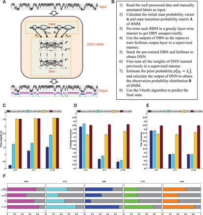
Development and performance assessment of the DNN–HMM algorithm. (A) Diagram of the DNN–HMM algorithm. In the DNN–HMM hybrid architecture, the HMM models the sequential property of the replication timing signal obtained from Repli-Seq data, and the DNN models the scaled observation likelihood probability distribution. (B) Pseudocode of the main steps to train the DNN–HMM. (C–E) Performance comparisons in terms of the computation time (C), training accuracy (D) and test accuracy (E) between the DNN–HMM algorithm and the three additional algorithms that we have implemented. ‘n = 0’ means that we use the original six-dimensional Repli-Seq data as inputs, ‘n = 5’ means that we concatenate five neighbours on both sides of the original, and ‘n = 10’ means that we concatenate 10 neighbours on both sides of the original. (F) Proportion of the replication domains of each type that are reproduced from another independent biological replicate of the Repli-Seq data in BJ cells by employing four algorithms
2.3 Identification of replication domains using DNN–HMM
We used Repli-Seq data to derive four different types of replication domains, including the ERD, the DTZ, the LRD and the UTZ. Inspired by the strategy used in the speech recognition field (Dahl et al., 2012), we refined each of the four domain types into three sub-domains. For example, we subdivided ERD into pre-ERD, mid-ERD and post-ERD. In addition, we added two additional domain types, the biphasic replication domain (BRD) and the dead zone (DZ). The BRD is the genomic region associated with simultaneous early and late replication, and the DZ is the zone without any Repli-Seq signals of six cell cycle fractions and is mainly located near the centromere. In total, we defined 14 states for replication domains.
According to the visualization of the Repli-Seq data through UCSC Genome Browser (http://genome.ucsc.edu/), we independently constructed the training and test sets by manually labelling the 14 states on chr1 and chr20 of BJ cell line of Replicate 1, respectively (Supplementary Fig. S1 and Supplementary Data). Considering the rareness of BRD on chr1 and chr20, we added several chromatin fragments manually labelled as BRD on other chromosomes to the training and test sets.
With the preparation of the training and test sets complete, we used the percentage-normalized signals of Repli-Seq data from six cell cycle fractions in BJ cells (Replicate 1) as input features to train our DNN–HMM algorithm, which consists of an input layer with six units, two hidden layers, both with 500 hidden units and an output layer with 14 units. The DNN–HMM outputs both the learned 261 014 model parameters and the predicted replication states of the training data. The learned model parameters were then used to assess the performance of our DNN–HMM algorithm in the analysis of the independent test data and in the prediction of the states of unlabelled data. The training and test accuracies were calculated for the training and test sets, respectively.
After assessing our DNN–HMM method, we merged the initially identified 14 sub-states into six types of replication domains: the ERD, the DTZ, the LRD, the UTZ, the BRD and the DZ. In the subsequent analysis, we focus on the first four types of replication domains.
2.4 Performance evaluation of the DNN–HMM
Although few bioinformatics methods have been specifically proposed for the de novo identification of replication domains using replication timing profiles, we identified six methods that have been developed in similar fields. In a previous study, Hansen et al. (2010) defined very ERD s with the G1 profile from Repli-Seq data. In another study, Ryba et al. (2010) identified replication domains by circular binary segmentation (Venkatraman and Olshen, 2007) using HD2 microarray data and identified timing transition regions (TTRs) from loess-smoothed replication timing profiles. These TTRs can be viewed similarly to our DTZs and UTZs, which connect early and LRDs. In a recent study, Pope et al. (2014) subdivided IMR90 topologically associated domains (TADs) into three classes (‘early’, ‘TTR’ and ‘late’) depending on both the means and standard deviations of the IMR90 replication timing within each TAD. We extended the TADs to the whole human genome and identified the early, TTR, and late domains strictly according to their definition. During the pilot phase of the ENCODE project, Thurman et al. combined an HMM with wavelet smoothing to produce a two-label segmentation of the ENCODE pilot regions into ‘active’ and ‘repressed’ regions (Birney et al., 2007; Thurman et al., 2007). This method was later developed into a tool named HMMSeg (Day et al., 2007). In the second phase of the ENCODE project, two research groups within the consortium independently developed algorithms for the annotation of the chromatin state, ChromHMM (Ernst and Kellis, 2010, 2012) and Segway (Hoffman et al., 2012). For these three unsupervised learning methods, we annotated the three states with ‘ERD’, ‘LRD’ and ‘TTR’ with replication timing profiles.
Based on these six reported methods, we computed the following performance indicators to compare the performance of these methods with that of our DNN–HMM.
| (6) |
| (7) |
where GM is the geometric mean of sensitivity and specificity, Sensitivity = TP/(TP + FN) and Specificity = TN/(TN + FP), and
| (8) |
where Recall = Sensitivity and Precision = TP/(TP + FP).
2.5 Integrative analysis of distinct types of replication domains
Detailed descriptions of the integrative analysis of distinct types of replication domains, including genomic annotations, statistical analysis by genome structure correction, motif enrichment analysis, density profiles surrounding the replication domains, enrichment analysis of TFs and Hi-C data analysis can be found in the Supplementary Methods.
3 Results
3.1 Development and performance assessment of the DNN–HMM
To identify the replication domains with Repli-Seq data de novo, we developed a hybrid architecture (DNN–HMM), integrating a DNN and a multivariate HMM (Fig. 1A and B). In the DNN–HMM architecture, the HMM models the sequential patterns of Repli-Seq data, and the DNN models the observation probability distribution. This approach combines the advantages of both HMM and DNN and has excellent potential for de novo discovery of ‘chromatin states’. To assess the performance of our DNN–HMM algorithm, we additionally developed a basic DNN algorithm and two classical GMM–HMM methods, including K-means GMM–HMM and EM GMM–HMM, independently.
To train and assess these four algorithms, we first constructed the training and test sets independently using UW Repli-Seq data in BJ cells (Hansen et al., 2010) (see ‘Methods’ section). For the training and test process, we used six-dimensional normalized Repli-Seq data in the training and test sets as input features and the manually annotated 14 sub-states of replication domains as input labels to train and test the four approaches. All of these algorithms were run on a computer with four CPU cores, Intel Core i7-4770 3.4 GHz, and 32 GB RAM. We repeated the training and test procedure 10 times with random initiation, independently. For each training and test, we recorded the computing time and calculated the prediction accuracies of the training set and test set (Fig. 1C–E, denoted by ‘n = 0’). As expected, the computing time of the two GMM–HMM algorithms were much faster than those of the two DNN algorithms. K-means GMM–HMM and EM GMM–HMM achieved much higher training accuracy (83.1 and 86.9%); however, they obtained much lower test accuracy (78.1 and 78.1%). These findings indicate that both GMM–HMMs are likely to encounter over-fitting problems. In contrast, both basic DNN and DNN–HMM achieved consistent training and test accuracies, suggesting that DNNs can efficiently resolve the over-fitting problem. Importantly, compared with the basic DNN algorithm, our DNN–HMM algorithm achieved the second-highest training accuracy (85.1%) and the highest test accuracy (84.6%).
To further assess the performance of these four methods in dealing with high-dimensional data, we increased the dimensionality of the input data by concatenating five sets of neighbour data on both sides of the original data. Thus, we used the (2 × 5 + 1) × 6 = 66-dimensional data as input data to train and test the four algorithms (Fig. 1C–E, denoted by ‘n = 5’). We found that the training and test accuracies of the two GMM–HMMs decreased rapidly and were <50%. In contrast, the increase of the dimensionality of the input data had almost no effect on both DNN algorithms, which have the highest training and test accuracies. In addition, consistent results were obtained when increasing the dimensionality of the input data to (2 × 10 + 1) × 6 = 126 by concatenating 10 neighbour data on both sides of the original (Fig. 1C–E, denoted by ‘n = 10’).
To evaluate the reproducibility of these methods, we repeated the de novo discoveries of distinct types of replication domains for two biological replicates of Repli-Seq data (BR1 and BR2) in BJ cells (Fig. 1F and Supplementary Table S2). Plotting distributions of replication timing profiles across the genomes of two BJ replicates shows a high correlation for these two replicates (Supplementary Fig. S2, ρ2 = 0.8983, P-value = 0). For distinct replication domains identified using DNN–HMM and another three approaches with Repli-Seq data of BR1 and BR2 in BJ cells, we found that the latter three cannot recover the de novo discoveries of replication domains from another independent replicate of BJ cells very well. In contrast, our DNN–HMM algorithm can recover the de novo discoveries of distinct types of replication domains well. In total, over 82% of replication domains of each type identified with DNN–HMM are shared and common between the two independent replicates in BJ cells. Such a significant degree of overlap (empirical P-value < 1.0 × 10⁻⁶) indicates that the distinct replication domains identified using DNN–HMM algorithms are reliable and robust. These performance assessments demonstrated that our DNN–HMM algorithm illustrates its superior robustness and greater representational power of data and achieves substantial improvements over discriminatively trained GMM–HMMs.
3.2 Comparison of the performance of the DNN–HMM with that of existing methods
We compared our DNN–HMM with the six above-mentioned methods based on four performance indicators: accuracy, GM, F1-score and reproducibility. Table 1 summarizes the comparative analysis of the performance of our method with that of the existing methods. For the identification of ERDs, our DNN–HMM method always performed better than all of the other methods, as determined based on the four performance indicators. For the identification of LRDs, DNN–HMM and Segway shared the best results, followed by ChromHMM, the method proposed by Pope et al., HMMSeg, the method proposed by Hansen et al. and the method proposed by Ryba et al. For the identification of TTRs, DNN–HMM was ranked first based on the GM, F1-score and reproducibility indicators and was ranked second based on the accuracy indicator.
Table 1.
Comparison of the performance of the DNN–HMM with that of existing methods
| Method | Domain type | performance indicators |
|||
|---|---|---|---|---|---|
| Accuracy (%) | GM (%) | F1-score (%) | Reproducibility (%) | ||
| DNN-HMM | ERD | 84.62 | 88.22 | 79.93 | 83.47 |
| LRD | 76.59 | 81.64 | 48.53 | 89.57 | |
| TTR | 87.26 | 74.76 | 49.67 | 79.04 | |
| Hansen et al. | ERD | 82.84 | 78.70 | 71.41 | 71.33 |
| LRD | Null | Null | Null | Null | |
| TTR | Null | Null | Null | Null | |
| Ryba et al. | ERD | Null | Null | Null | Null |
| LRD | Null | Null | Null | Null | |
| TTR | 89.67 | 62.56 | 44.66 | 56.78 | |
| Pope et al. | ERD | 82.23 | 83.72 | 75.19 | 65.29 |
| LRD | 78.23 | 79.62 | 48.12 | 79.58 | |
| TTR | 75.64 | 62.18 | 29.04 | 41.25 | |
| HMMSeg | ERD | 82.79 | 84.08 | 75.73 | 59.32 |
| LRD | 76.22 | 78.02 | 45.61 | 46.29 | |
| TTR | 73.40 | 66.26 | 30.83 | 47.53 | |
| ChromHMM | ERD | 81.24 | 81.83 | 73.14 | 75.33 |
| LRD | 79.12 | 81.40 | 50.08 | 63.54 | |
| TTR | 68.78 | 59.82 | 24.70 | 64.08 | |
| Segway | ERD | 82.81 | 84.09 | 75.75 | 57.43 |
| LRD | 81.15 | 80.53 | 51.16 | 73.68 | |
| TTR | 73.14 | 65.64 | 30.27 | 50.85 | |
TTR is the union set of DTZ and UTZ. ‘Null’ indicates that the method cannot be used to identify the corresponding type of replication domain.
Because the different performance indicators demonstrate the distinct advantages and disadvantages of these studied methods, we ranked their performance according to the four metrics. In total, we performed 12 different tests, including seven methods, three types of identification domains and four performance indicators. Based on the ideas proposed by Bajic (2000), we obtained the average of the ranked positions of each of the seven methods in all of the 12 tests. Table 2 illustrates the overall score and average rank position of each of the methods. A lower average rank indicates a better performance. The analysis revealed that across the different performance tests, the DNN–HMM was ranked first, followed by Segway, ChromHMM, the method proposed by Pope et al., HMMSeg, the method proposed by Ryba et al. and the method proposed by Hansen et al. This result convincingly demonstrates that DNN–HMM performs well relative to the existing methods for the identification of replication domains.
Table 2.
Relative ranking of DNN–HMM and existing methods based on results of our comparison study
| Performance indicators | Domain type | DNNHMM | Hansen et al. | Ryba et al. | Pope et al. | HMMSeg | ChromHMM | Segway |
|---|---|---|---|---|---|---|---|---|
| Accuracy | ERD | 1 | 2 | 7 | 5 | 4 | 6 | 3 |
| LRD | 4 | 6 | 6 | 3 | 5 | 2 | 1 | |
| TTR | 2 | 7 | 1 | 3 | 4 | 6 | 5 | |
| GM | ERD | 1 | 6 | 7 | 4 | 3 | 5 | 2 |
| LRD | 1 | 6 | 6 | 4 | 5 | 2 | 3 | |
| TTR | 1 | 7 | 4 | 5 | 2 | 6 | 3 | |
| F1-score | ERD | 1 | 6 | 7 | 4 | 3 | 5 | 2 |
| LRD | 3 | 6 | 6 | 4 | 5 | 2 | 1 | |
| TTR | 1 | 7 | 2 | 5 | 3 | 6 | 4 | |
| Reproducibility | ERD | 1 | 3 | 7 | 4 | 5 | 2 | 6 |
| LRD | 1 | 6 | 6 | 2 | 5 | 4 | 3 | |
| TTR | 1 | 7 | 3 | 6 | 5 | 2 | 4 | |
| Overall ranking | 1st (18), 1.50 | 6th (69), 5.75 | 5th (62), 5.17 | 4th (49), 4.08 | 4th (49), 4.08 | 3rd (48), 4.00 | 2nd (37), 3.08 | |
TTR is the union set of DTZ and UTZ. In the last line, we illustrate the relative ranking order of the method based on the results for the four performance indicators analysed in our comparison study.
3.3 Identification and characterization of distinct replication domains
We applied our trained DNN–HMM to the de novo identification of genome-wide replication domains across 15 human cell types using UW Repli-Seq data (Hansen et al., 2010) in the ENCODE project. The four types of replication domains differ substantially in their genome coverage, genome location, numbers of domains, numbers of genes, evolutionary conservation, cell type-specificity and replication timing features (see Supplementary Material; Supplementary Fig. S3 and Supplementary Data).
To investigate the occupancy signatures of TFs within each type of replication domain, we identified sequence features that characterize distinct replication domains. We used a collection of in vitro motifs that represent the binding preferences of 492 human TFs and determined the relative enrichment significance of TF-binding elements within diverse replication domains (Supplementary Fig. S4 and Supplementary Data). We noticed that a vast majority of these TF-binding motifs (469 of 492, 95.3%) were significantly enriched in at least one type of replication domain. Among the 192 of 469 TFs (40.9%) enriched within the ERDs, KLF4, MYC, SMAD3, TP53, E2F1, EGR1, SP1 and YY1 have been explicitly reported to play important roles in the control of the G1/S-phase transition of the cell cycle, and others, such as MAZ and E4F1, have been reported to be closely associated with cell cycle activity (Supplementary Table S5). Two hundred and two (43.1%) TFs, including TBX18, CUX1, GATA6, HNF1A, IK2F2, MSX2, POU5F1, SOX2, CDC5L, ALX1 and ESX1, were specifically enriched within LRDs. It has been reported that CDC5L, ESX1 and GATA6 play important roles in the control of the G2 and M phases of the cell cycle and that CUX1 and ALX1 play important roles in cell cycle progression (Supplementary Table S5). DTZs and UTZs demonstrate similar enrichment of TFs, which are enriched in either ERDs or LRDs. We found that a small fraction of TFs (75 of 469, 16.0%) were significantly enriched in all of these types of replication domains. These factors include DDIT3, NANOG and STAT1, which have also been reported to play important roles in the cell cycle (Supplementary Table S5).
To further quantify the occupancy relationship between distinct replication domains and the regulatory factors, we compiled ChIP-Seq data from ENCODE of 8, 13 and 5 different TFs and cofactors in IMR90, GM12878 and K562 cells (Supplementary Fig. S5). We compared their accumulated normalized intensities with those from regions immediately outside the domains (to the left and to the right) and with those determined from randomly shuffled domains. This analysis showed that all of the examined TFs and cofactors, with the exception of ZNF274, were significantly enriched in ERDs and differentially depleted in LRDs, whereas ZNF274 were significantly enriched in LRDs and differentially depleted in ERDs (Supplementary Fig. S6). A further enrichment analysis of the TF and cofactor peaks with different replication domains confirmed the enrichment and depletion patterns of TFs and cofactors within each type of replication domain (Supplementary Fig. S7). Among the TFs and cofactors enriched in ERDs, studies have explicitly reported that RAD21, E2F4, BRCA1, CJUN, GATA1, STAT3, CMYC, TP53, EGR1, SP1, YY1 and BACH1 play important roles in G1/S cell cycle progression (Supplementary Table S5). In addition, a recent study has demonstrated that the zinc-finger protein ZNF274 associates with the histone H3 lysine 9 (H3K9) methyltransferase SETDB1, which is recruited by MDB1 to CAF-1 to form an S phase-specific CAF-1/MDB1/SETDB1 complex during DNA replication (Supplementary Table S5). Notably, we found that within each type of replication domain, the enrichment and depletion patterns obtained with motif scanning agree well with those obtained from ChIP-Seq data for the TFs that have in vitro motifs (Supplementary Fig. S4 and Supplementary Data). These TFs include CTCF, EP300, MAZ, CEBPB, TP53, YY1, BHLHE40, NRF1, MAX, ELK1, STAT3, USF2, SP1, EGR1, BACH1, CMYC and ZNF263, which play essential roles in the cell cycle. Furthermore, we found that CTCF and CEBPB were both enriched in DTZs and UTZs (Supplementary Fig. S7 and Supplementary Data). Together, these findings suggest that distinct replication domains possess unique sequence features.
To delineate the nature of each type of replication domain, we analysed the chromatin signatures in distinct replication domains. We examined 10 histone modifications (H3K4me1/me2/me3, H3K36me3, H3K27me3, H3K9me3, H3K79me2, H4K20me1, H3K9ac and H3K27ac), one histone variant (H2A.Z), DNA methylation, RNA polymerase II, RNA signals, DNase I hypersensitive sites (DHSs) and nuclear lamina (see Supplementary Fig. S8). These data represent different types of chromatin activities from human IMR90 cells. We compared the aggregate normalized density profiles between distinct types of replication domains as we did for TFs and cofactors. We found that ERDs and LRDs showed unique enrichment and depletion patterns within the replication domains and at the boundaries for each chromatin marker, respectively (Supplementary Fig. S9). This finding is consistent with those obtained in previous studies. A further colocalization analysis and correlation analysis between ERDs and LRDs and chromatin markers demonstrated that the unique enrichment and depletion patterns specifically dependent on the cell type (Supplementary Figs. S10 and Supplementary Data). Together, our findings demonstrate that early and late replication are linked to active and repressive chromatin markers in a cell type-specific manner, respectively. Notably, early-replicating regions are more highly methylated than late-replicating regions.
3.4 Chromatin architecture of distinct replication domains
Recent studies have revealed the association between replication timing and higher-order chromosomal structure (Pope et al., 2014; Ryba et al., 2010). Our analysis further strengthens these tight associations in distinct types of replication domains (see Supplementary Fig. S12). We then investigated the chromatin interactions between intra- and inter-replication domains (Supplementary Fig. S13A–C), and found that interactions within each type of replication domain were enriched but that interactions between different types of replication domains are depleted (Supplementary Figs. S13A–C). This finding indicates that the entire genome can be partitioned into different types of replication domains such that greater interaction occurs within each type of replication domain rather than across distinct types of replication domains. Furthermore, domains within each type of replication domain are more densely packed internally, with LRD being the densest and ERD the loosest (Supplementary Fig. S13A). Notably, we found that inter-interaction between DTZs and UTZs was higher than the inter-interaction within DTZs and UTZs (Supplementary Figs. S13B and Supplementary Data, P-value < 1.0 × 10⁻¹⁹), implying that DTZs and UTZs tend to colocalize. Thus, we hypothesized that the adjacent DTZ–UTZ pairs separated by ERDs and LRDs contact much more closely and may form a chromatin loop. To test this hypothesis, we examined the interactions between adjacent DTZ–UTZ pairs on both sides of ERDs or LRDs (Supplementary Fig. S13D). We found that the inter-interactions between adjacent DTZ–UTZ pairs separated by LRDs were significantly stronger than the inter-interaction between adjacent DTZ–UTZ pairs separated by an ERD. Furthermore, the interactions between adjacent DTZ–UTZ pairs separated by ERDs were markedly stronger than the intra-interaction within ERDs, and the interactions between adjacent DTZ–UTZ pairs separated by LRDs were also comparable with the intra-interaction within LRDs (Supplementary Fig. S13A and Supplementary Data), although the genomic distance between adjacent DTZ–UTZ pairs was much larger than those of internal loci within ERDs or LRDs. To further demonstrate our hypothesis, we fixed one side of the adjacent DTZ–UTZ pairs and examined the inter-interactions between this side with another side and its flanking regions (Fig. 2A and B). We found that the interactions of adjacent DTZ–UTZ pairs were substantially stronger than those of flanking regions. Furthermore, we explored the interactions between the adjacent DTZ–UTZ pairs and their flanking regions by keeping the distance of the adjacent DTZ–UTZ pairs constant (Fig. 2C). The interactions of the adjacent DTZ–UTZ pairs were highest in the interaction profiles. These findings suggest that adjacent DTZ–UTZ pairs separated by ERDs and LRDs closely colocalize and provide compelling evidence that the adjacent DTZ–UTZ pairs form a chromatin loop.
Fig. 2.

Genome-wide chromatin interactions of replication domains. (A–B) Interaction profiles surrounding the adjacent DTZ–UTZ pair obtained by fixing one side (anchor) of the pair that encloses ERDs (A) and LRDs (B). (C) Interaction profiles surrounding the adjacent DTZ–UTZ pair obtained by keeping the distance of the adjacent DTZ–UTZ pairs constant. (D) Intra-interaction I(s) for pairs of loci separated by a genomic distance s within ERDs (magenta), LRDs (blue) and randomly shuffled regions (grey). (E) Distribution of genomic spans of all chromatin interactions below the threshold I(s) ≥ 0 within ERDs (magenta) and LRDs (blue). (F) Median genomic spans of the distance distributions of all chromatin interactions below any thresholds within ERDs (magenta) and LRDs (blue)
We then closely examined the chromatin interactions in the vicinity of the centre of each type of replication domain (Supplementary Fig. S13E–H). Strikingly, we found that a locus within ERDs mainly interacts with a close intra-locus, whereas a locus within LRDs mainly interacts with a far intra-locus (Supplementary Fig. S13E and Supplementary Data). Based on this observation, we hypothesize that intra-interactions within each ERD tend to be short-range, where intra-interactions within each LRD prefer to be long-range. To test this hypothesis, we calculated the average intra-interaction I(s) for pairs of loci separated by a genomic distance s within ERDs and LRDs (Fig. 2D). We found that as the genomic distance s increased, the average intra-interaction I(s) within ERDs increased over a very short genomic distance and then decreased markedly, whereas the average intra-interaction I(s) within LRDs decreased over a very short genomic distance and then increased substantially. To further assess the short- and long-range interactions, we measured the distributions of genomic distance s at the threshold of interaction I(s) ≥ 0 within ERDs and LRDs, respectively (Fig. 2E). We observed that the median interaction distance within ERDs was markedly smaller than that within LRDs. We extended this analysis for any given threshold of interaction I(s), and plotted the curves of the median interaction distances within ERDs and LRDs (Fig. 2F). The median interaction distance within the LRDs was always markedly larger than the median interaction distance within the ERDs. These results support the hypothesis that intra-interactions within ERDs tend to be short-range and that intra-interactions within LRDs are likely to be long-range.
4 Discussion
In this study, we propose a pre-trained DNN–HMM hybrid model and present its first successful application for de novo identification of replication domains with replication timing profiles from Repli-Seq data. Our approach has two key characteristics that distinguish it from earlier methods. First, we adopted a deeper, more expressive DNN–HMM hybrid architecture and thus employed the unsupervised DBN pre-training and subsequent supervised fine-tuning strategy, which made the training more effective. Second, we used posterior probabilities of states as the output of DNN, which made the training more informative. Subsequent performance assessments demonstrated that our DNN–HMM approach achieves substantial improvements in identification accuracy and robustness over discriminatively trained pure GMM–HMM systems, generatively trained traditional DNN algorithms and other six reported methods.
Despite these promising results, there are many aspects of using DNN–HMM for practical scalability in computational biology that require further study. These aspects include investigation of the parallelization of DNN training, which may require a better theoretical understanding of deep learning, and the exploration of more optimal algorithms to training DNN–HMM rather than the embedded suboptimal Viterbi algorithm. There is also a need to explore the vast improvement space in the DNN–HMM hybrid model, including adopting a full-sequence training of the DBN, using the mean–covariance RBM, and even absorbing the insights gained from generative modelling research in both neural networks and speech and phone recognition.
Recently, Brendan J. Frey and his colleagues applied a DNN to investigate the human and mouse splicing codes and demonstrated the superior advantages of this deep architecture over the previous Bayesian method for predicting the patterns of alternative splicing (Leung et al., 2014; Xiong et al., 2015). Compared with their DNN structure of a two-layer neural network with only 30 hidden units, our DNN–HMM hybrid architecture is much more complex and flexible. Regardless, their work and ours represent a critical process of applying deep learning in computational biology. In particular, with the exponentially rapid growth in the volume of multi-omic data, such as genomics, transcriptomics, epigenomics, proteomics and chromatin interactomics, our hybrid architecture employing DNN and HMM has the potential to produce meaningful and hierarchical representations that can be efficiently used to describe complex biological phenomena. For example, DNN–HMMs may be useful for modelling multiple stages of a regulatory network at the sequence level and at higher levels of abstraction. In addition, DNN–HMM can be applied to the identification of functional elements and regions, such as enhancers, insulators and promoters, and the identification of chromatin states.
We applied our DNN–HMM algorithm to de novo identification of distinct types of replication domains, including ERD, DTZ, LRD and UTZ, using Repli-Seq data across 15 human cell types. We performed a systematic and integrative analysis of these domains using diverse ENCODE data and unravelled the replication domains of distinct types that harbour unique genomic and epigenetic patterns, transcriptional activity and higher-order chromosomal structure. Our results support a unifying model in which the human genome is generally organized into large replication domains of distinct types that constitute stable regulatory units of replication timing. In our ‘replication-domain model’ (Fig. 3), DNA replicates early within ERDs that acquire permissive chromatin signatures and active regulators. Meanwhile, replication gradually moves forward into adjacent LRDs that contain repressive chromatin features and repressive regulators. This gradual progression forms DTZs or UTZs that connect the boundaries of ERDs and LRDs. DTZs were characterized by the sharp decrease/increase of active/repressive chromatin markers, whereas UTZs were characterized by the sharp increase/decrease of active/repressive chromatin markers.
Fig. 3.

The replication domain model. Model of chromosome organization during DNA replication. This model was obtained by summarizing the main results presented in this study. Large, discrete replication domains (ERDs and LRDs) demarcated by DTZs and UTZs are spatially compartmentalized structural and functional units of higher-order chromosomal structure and are dynamically associated with the nuclear lamina. In this model, the ERD is an open, loosely packed, transcriptionally active chromatin domain located far from the nuclear membrane and occupied by active epigenetic markers and active regulators, whereas the LRD is a closed, densely packed, transcriptionally inactive chromatin domain located near the nuclear membrane and occupied by repressive epigenetic markers and repressive regulators. The ERD and LRD are spatially separated by the DTZ and UTZ, which are transition zones enriched with H3k27me3 and occupied by CTCF. The adjacent DTZ–UTZ pairs form chromatin loops, and intra-interactions within ERDs and LRDs tend to be short- and long-range, respectively
Our replication-domain model agrees well with the previously presented fractal globule, a knot-free, polymer conformation (Lieberman-Aiden et al., 2009). In our model, spatially separated fractal globules are equivalent to temporally separated ERDs and LRDs that are connected by UTZs and DTZs. The adjacent DTZ–UTZ pairs separated by an ERD or LRD form a chromatin loop for each ERD and LRD through the acquisition of much stronger contacts. Most importantly, we found that in the chromatin loops formed by adjacent DTZ–UTZ pairs, LRDs prefer to be more densely packed and in long-range intra-interactions, whereas ERDs tend to be more loosely packed and in short-range intra-interactions.
Supplementary Material
Acknowledgements
We wish to thank the ENCODE Project Consortium for making their data publicly available. We thank Dr. Yu Dong (the Speech Research Group, Microsoft Research, Redmond, WA 98034, USA) for constructive suggestions and comments regarding our DNN–HMM method.
Funding
This work was supported by grants from the Major Research plan of the National Natural Science Foundation of China (No. U1435222), the Program of International S&T Cooperation (No. 2014DFB30020) and the National High Technology Research and Development Program of China (No. 2015AA020108).
Conflict of Interest: none declared.
References
- Audit B., et al. (2007) DNA replication timing data corroborate in silico human replication origin predictions. Phys. Rev. Lett., 99, 248102. [DOI] [PubMed] [Google Scholar]
- Bajic V.B. (2000) Comparing the success of different prediction software in sequence analysis: a review. Brief. Bioinform., 1, 214–228. [DOI] [PubMed] [Google Scholar]
- Bell S.P., Dutta A. (2002) DNA replication in eukaryotic cells. Annu. Rev. Biochem., 71, 333–374. [DOI] [PubMed] [Google Scholar]
- Bengio Y. (2009) Learning Deep Architectures for AI. Now Publishers Inc., Hanover. [Google Scholar]
- Bengio Y., et al. (2013) Representation learning: a review and new perspectives. IEEE Trans. Patt. Anal. Mach. Intell., 35, 1798–1828. [DOI] [PubMed] [Google Scholar]
- Bicknell L.S., et al. (2011a) Mutations in the pre-replication complex cause Meier-Gorlin syndrome. Nat. Genet., 43, 356–359. [DOI] [PMC free article] [PubMed] [Google Scholar]
- Bicknell L.S., et al. (2011b) Mutations in ORC1, encoding the largest subunit of the origin recognition complex, cause microcephalic primordial dwarfism resembling Meier-Gorlin syndrome. Nat. Genet., 43, 350–355. [DOI] [PubMed] [Google Scholar]
- Birney E., et al. (2007) Identification and analysis of functional elements in 1% of the human genome by the ENCODE pilot project. Nature, 447, 799–816. [DOI] [PMC free article] [PubMed] [Google Scholar]
- Dahl G.E., et al. (2012) Context-dependent pre-trained deep neural networks for large-vocabulary speech recognition. IEEE Trans. Audio Speech, 20, 30–42. [Google Scholar]
- Day N., et al. (2007) Unsupervised segmentation of continuous genomic data. Bioinformatics (Oxford, England), 23, 1424–1426. [DOI] [PubMed] [Google Scholar]
- Erhan D., et al. (2010) Why does unsupervised pre-training help deep learning? J. Mach. Learn. Res., 11, 625–660. [Google Scholar]
- Ernst J., Kellis M. (2010) Discovery and characterization of chromatin states for systematic annotation of the human genome. Nat. Biotechnol., 28, 817–825. [DOI] [PMC free article] [PubMed] [Google Scholar]
- Ernst J., Kellis M. (2012) ChromHMM: automating chromatin-state discovery and characterization. Nat. Methods., 9, 215–216. [DOI] [PMC free article] [PubMed] [Google Scholar]
- Farkash-Amar S., et al. (2008) Global organization of replication time zones of the mouse genome. Genome Res., 18, 1562–1570. [DOI] [PMC free article] [PubMed] [Google Scholar]
- Guernsey D.L., et al. (2011) Mutations in origin recognition complex gene ORC4 cause Meier-Gorlin syndrome. Nat. Genet., 43, 360–364. [DOI] [PubMed] [Google Scholar]
- Hansen R.S., et al. (2010) Sequencing newly replicated DNA reveals widespread plasticity in human replication timing. Proc. Natl Acad. Sci. U.S.A., 107, 139–144. [DOI] [PMC free article] [PubMed] [Google Scholar]
- Hinton G. (2009) Deep belief networks. Scholarpedia, 4, 5947. [Google Scholar]
- Hinton G.E., et al. (2006) A fast learning algorithm for deep belief nets. Neural Comput., 18, 1527–1554. [DOI] [PubMed] [Google Scholar]
- Hinton G.E., Salakhutdinov R.R. (2006) Reducing the dimensionality of data with neural networks. Science, 313, 504–507. [DOI] [PubMed] [Google Scholar]
- Hoffman M.M., et al. (2012) Unsupervised pattern discovery in human chromatin structure through genomic segmentation. Nat. Methods, 9, 473–476. [DOI] [PMC free article] [PubMed] [Google Scholar]
- Karnani N., et al. (2007) Pan-S replication patterns and chromosomal domains defined by genome-tiling arrays of ENCODE genomic areas. Genome Res., 17, 865–876. [DOI] [PMC free article] [PubMed] [Google Scholar]
- Letessier A., et al. (2011) Cell-type-specific replication initiation programs set fragility of the FRA3B fragile site. Nature, 470, 120–123. [DOI] [PubMed] [Google Scholar]
- Leung M.K., et al. (2014) Deep learning of the tissue-regulated splicing code. Bioinformatics (Oxford, England), 30, i121–i129. [DOI] [PMC free article] [PubMed] [Google Scholar]
- Lieberman-Aiden E., et al. (2009) Comprehensive mapping of long-range interactions reveals folding principles of the human genome. Science, 326, 289–293. [DOI] [PMC free article] [PubMed] [Google Scholar]
- Lucas I., et al. (2007) High-throughput mapping of origins of replication in human cells. EMBO Rep., 8, 770–777. [DOI] [PMC free article] [PubMed] [Google Scholar]
- MacAlpine D.M., et al. (2004) Coordination of replication and transcription along a Drosophila chromosome. Genes Dev., 18, 3094–3105. [DOI] [PMC free article] [PubMed] [Google Scholar]
- Masai H., et al. (2010) Eukaryotic chromosome DNA replication: where, when, and how? Annu. Rev. Biochem., 79, 89–130. [DOI] [PubMed] [Google Scholar]
- Pope B.D., et al. (2014) Topologically associating domains are stable units of replication-timing regulation. Nature, 515, 402–405. [DOI] [PMC free article] [PubMed] [Google Scholar]
- Raghuraman M.K., et al. (2001) Replication dynamics of the yeast genome. Science, 294, 115–121. [DOI] [PubMed] [Google Scholar]
- Ryba T., et al. (2010) Evolutionarily conserved replication timing profiles predict long-range chromatin interactions and distinguish closely related cell types. Genome Res., 20, 761–770. [DOI] [PMC free article] [PubMed] [Google Scholar]
- Schubeler D., et al. (2002) Genome-wide DNA replication profile for Drosophila melanogaster: a link between transcription and replication timing. Nat. Genet., 32, 438–442. [DOI] [PubMed] [Google Scholar]
- Schwaiger M., et al. (2009) Chromatin state marks cell-type- and gender-specific replication of the Drosophila genome. Genes Dev., 23, 589–601. [DOI] [PMC free article] [PubMed] [Google Scholar]
- Sclafani R.A., Holzen T.M. (2007) Cell cycle regulation of DNA replication. Annu. Rev. Genet., 41, 237–280. [DOI] [PMC free article] [PubMed] [Google Scholar]
- Suzuki M., Takahashi T. (2013) Aberrant DNA replication in cancer. Mut. Res., 743–744, 111–117. [DOI] [PubMed] [Google Scholar]
- Thurman R.E., et al. (2007) Identification of higher-order functional domains in the human ENCODE regions. Genome Res., 17, 917–927. [DOI] [PMC free article] [PubMed] [Google Scholar]
- Venkatraman E.S., Olshen A.B. (2007) A faster circular binary segmentation algorithm for the analysis of array CGH data. Bioinformatics (Oxford, England), 23, 657–663. [DOI] [PubMed] [Google Scholar]
- Woo Y.H., Li W.H. (2012) DNA replication timing and selection shape the landscape of nucleotide variation in cancer genomes. Nat. Commun., 3, 1004. [DOI] [PubMed] [Google Scholar]
- Woodfine K., et al. (2005) Replication timing of human chromosome 6. Cell Cycle, 4, 172–176. [DOI] [PubMed] [Google Scholar]
- Xiong H.Y., et al. (2015) RNA splicing. The human splicing code reveals new insights into the genetic determinants of disease. Science, 347, 1254806. [DOI] [PMC free article] [PubMed] [Google Scholar]
Associated Data
This section collects any data citations, data availability statements, or supplementary materials included in this article.