Abstract
The effects of signal and noise on contrast discrimination are difficult to separate because of a singularity in the signal-detection-theory model of two-alternative forced-choice contrast discrimination (Katkov, Tsodyks, & Sagi, 2006). In this article, we show that it is possible to eliminate the singularity by combining that model with a binocular combination model to fit monocular, dichoptic, and binocular contrast discrimination. We performed three experiments using identical stimuli to measure the perceived phase, perceived contrast, and contrast discrimination of a cyclopean sine wave. In the absence of a fixation point, we found a binocular advantage in contrast discrimination both at low contrasts (<4%), consistent with previous studies, and at high contrasts (≥34%), which has not been previously reported. However, control experiments showed no binocular advantage at high contrasts in the presence of a fixation point or for observers without accommodation. We evaluated two putative contrast-discrimination mechanisms: a nonlinear contrast transducer and multiplicative noise (MN). A binocular combination model (the DSKL model; Ding, Klein, & Levi, 2013b) was first fitted to both the perceived-phase and the perceived-contrast data sets, then combined with either the nonlinear contrast transducer or the MN mechanism to fit the contrast-discrimination data. We found that the best model combined the DSKL model with early MN. Model simulations showed that, after going through interocular suppression, the uncorrelated noise in the two eyes became anticorrelated, resulting in less binocular noise and therefore a binocular advantage in the discrimination task. Combining a nonlinear contrast transducer or MN with a binocular combination model (DSKL) provides a powerful method for evaluating the two putative contrast-discrimination mechanisms.
Keywords: nonlinear contrast transducer, contrast-gain control, interocular inhibition, interocular enhancement, anticorrelation, accommodation fluctuation, binocular advantage, fixation point, gain-control of gain-control, singularity
Introduction
Sensory discrimination depends on both the mean (signal) and variance (noise) of the sensory responses (Green & Swets, 1966). Typically, the discrimination performance (d′) depends on the signal-to-noise ratio, remaining constant when both signal and noise increase or decrease. However, with only discrimination measurements, it is difficult or even impossible to separate the effects of the signal and the noise on discrimination performance. For example, enhanced performance could be equally well accounted for by an increase in signal or a decrease in noise, resulting in a singularity in the signal-detection-theory (SDT) model of two-alternative forced-choice (2AFC) contrast-discrimination data (Katkov, Tsodyks, & Sagi, 2006). To avoid the singularity, a prior assumption is needed for fitting a model (Katkov et al., 2006). With an assumption of constant noise, the discrimination data can be accounted for by a nonlinear contrast transducer (NCT), such as monocular or binocular contrast-gain control. With an assumption of linear contrast transformation, the same data could also be accounted for by multiplicative noise (MN), in which the variance is dependent on stimulus. Despite a great deal of effort (e.g., Georgeson & Meese, 2006; Klein, 2006; Kontsevich, Chen, & Tyler, 2002), no previous study has succeeded in distinguishing between NCT and MN in contrast discrimination because of the singularity (Katkov et al., 2006).
However, it is possible to eliminate the singularity by using a binocular combination model to estimate the mean and variance of the binocular contrast response for each pair of contrast. Here is an example, contributed by an anonymous reviewer: Suppose we make only monocular measurements, and we find that our manipulation x causes d′ to double. This could be due to one of two possibilities: Before manipulation x, the mean response difference was 4 units and the noise standard deviation was 4 units, so that d′ = 4/4 = 1; after manipulation x, d′ could become 2 either because the mean response difference doubled (d′ = 8/4 = 2) or because internal noise halved (d′ = 4/2 = 2). Now suppose we carry out another manipulation y, and we find that d′ goes from 1 to 4; again, there are two possibilities: 16/4 = 4 and 4/1 = 4. With only the monocular measurement, every time we apply a manipulation and see a d′ change, we cannot know whether it is because the numerator goes up or the denominator goes down. But now we measure the output from both eyes, and we apply the two manipulations separately but simultaneously to both eyes. Suppose we know how the outputs from the two eyes are combined, and that they are simply summed. Now we apply manipulation x to one eye and manipulation y to the other. Under the hypothesis that our manipulations change mean response, the final d′ should be  . Under the hypothesis that the manipulations reduce noise standard deviation, it should be
  . So the two numbers are different, and we can tell them apart. More generally, we can apply a continuum for our manipulation, and if we plot all possible paired values between the two eyes, the resulting surface for binocular d′ will have a form that is different under the two hypotheses of changing mean response and changing noise standard deviation. Theoretically, through combining the SDT model and a binocular combination model the singularity could be removed and a unique solution obtained to the question of how the signal and noise affect contrast discrimination. For this purpose, we need a robust binocular combination model that works in multiple binocular tasks.
One candidate is a binocular model deduced from interocular contrast-gain-control theory, which was first developed to account for binocular phase combination (Ding & Sperling, 2006) and later modified to explain both phase and contrast combination in binocular vision (Ding, Klein, & Levi, 2013b; Huang, Zhou, Zhou, & Lu, 2010). To attempt a unified explanation of both contrast and phase data, Huang et al. (2010) added an extra contrast channel to the Ding–Sperling model, thus creating the Multiple Channel Model. However, the Multiple Channel Model has a major shortcoming: It is based on the assumption that binocular contrast summation is independent of the phase of the two eyes' sine waves, but this assumption is not consistent with experimental data at low contrast levels (Baker, Wallis, Georgeson, & Meese, 2012; Ding et al., 2013b). As an alternative, we tested the addition of interocular contrast enhancement and a sensory fusion mechanism to the Ding–Sperling model. The resulting DSKL model (Ding et al., 2013a, 2013b) offers a significant improvement: It successfully predicts both binocular phase and contrast combination using a single set of model parameters over a large range of input contrasts and phases in the two eyes in both normal and amblyopic observers. Model simulations show that, with the addition of an NCT and additive (independent of input) Gaussian noise, the Ding–Sperling model and the DSKL model capture the main features of binocular contrast discrimination. However, it is still unclear where to insert a contrast-discrimination mechanism in the binocular visual system. Our previous study (Ding et al., 2013c) showed that inserting an MN mechanism (which varies with input) before the site of binocular combination resulted in better performance in binocular contrast discrimination than inserting the noise after the binocular site, consistent with experimental data.
Another candidate is the two-stage model, which was first proposed to account for monocular, dichoptic, and binocular contrast discrimination (Meese, Georgeson, & Baker, 2006; Meese & Hess, 2004). The first stage of the model contains both monocular and interocular contrast-gain control, and the second stage contains binocular contrast-gain control followed by additive Gaussian noise. The same model was later used to explain a binocular contrast-matching task (Baker, Meese, & Georgeson, 2007). Assuming that the nonlinear operators in the model's signal path have no effect on the phase, the two-stage model can also explain binocular phase combination (Ding et al., 2013b). In this article, we compare the two-stage model, the Ding–Sperling model, and the DSKL model in explaining three sets of data: phase matching, contrast matching, and contrast discrimination.
Although it is theoretically possible to remove the singularity in the SDT model by combining it with a robust binocular combination model, without an analytic formula for the variance when the signal and noise go through a nonlinear operator, it is very difficult in practice to fit the combined model when early noise is added to the binocular visual system. Therefore, in this article, we first fit the binocular combination model to the binocular-combined phase- and contrast-matching data, and then insert the NCT or MN into this model with already-known parameters. We compare the NCT and MN mechanisms in two ways: (a) fitting both monocular and binocular contrast-discrimination data with a late noise (after all nonlinear operators), and (b) first fitting the two mechanisms to monocular contrast-discrimination data separately and then predicting binocular contrast-discrimination performance with an NCT or MN inserted into one of three locations (early, middle, or late) in the binocular system. The fit of the predictions to the experimental results suggests that the best model is an early MN inserted into the DSKL model.
Methods
The methods used in this article are almost identical to those of our previous studies (Ding et al., 2013a, 2013b).
Stimuli
Horizontal gratings with sinusoidal luminance profiles IL = I0L(1 + mLcos(2πfsy + θL)) and IR = I0R(1 + mRcos(2πfsy + θR)) were used as stimuli. I0L and I0R are the luminance of the background and the mean luminance of the sine-wave gratings in the two eyes (= 26.2 cd/m2); fs is the spatial frequency (= 0.68 c/°), identical in both eyes; mL and mR are the modulation contrasts of the left- and right-eye sine-wave gratings, respectively; and θL and θR are the corresponding phases. The stimuli were windowed in a circular window spatially with a blurred edge (3° in diameter) and a square window temporally (117 ms). The observation distance was 68 cm.
Procedure
The procedure for measuring the perceived phase and contrast of a cyclopean sine wave was identical to that used in our previous studies (Ding et al., 2013a, 2013b). Perceived phase was measured using phase-matching procedures modified from Ding and Sperling (2006). Each trial began with the presentation of a dichoptic nonius cross surrounded by a high-contrast frame (Figure 1, top panel). Once the dichoptic cross was perceived to be aligned and stable, the observer pressed a key to initiate the trial. Following the key press, a screen with only the surrounding high-contrast frame and reference horizontal lines appeared, for 500 ms, followed by sine-wave gratings presented to the two eyes respectively for 117 ms (Figure 1, bottom panel). Stimulus presentation was followed by a blank screen of mean luminance until the observer responded. The observer's task was to indicate the apparent location of the center of the dark stripe in the perceived cyclopean sine-wave grating, relative to a black horizontal reference line adjacent to its edge. The observer pressed one of two keys to indicate whether the reference line was judged to be above or below the dark cyclopean stripe. The physical position of the reference line was fixed, always in the center, to aid fixation, but its position relative to the dark cyclopean stripe was varied from trial to trial by shifting the phase of the two eyes' sine waves using a one-up-one-down staircase, in order to measure the perceived phase of the cyclopean sine wave.
Figure 1.
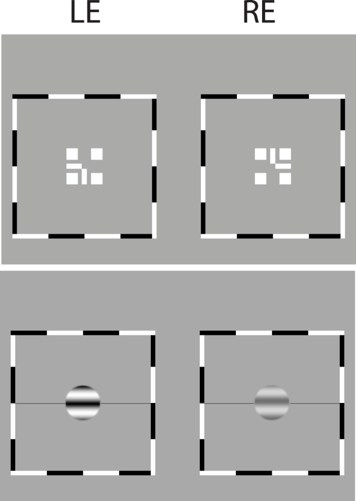
Stimuli. A dichoptic nonius cross surrounded by a high-contrast frame (top) and sine-wave gratings presented to the two eyes (bottom).
The perceived contrast of a cyclopean sine wave was measured using a contrast-matching task. The stimuli were identical to those used in the phase-matching experiment (Figure 1). The procedure was also similar, except for having two stimulus intervals, one with a standard contrast (48%, 24%, 12%, or 6%) only presented to the left eye (LE) and the other with a test contrast presented to both eyes with the interocular contrast ratio varying from trial to trial. Each interval lasted for 117 ms, and the interstimulus interval was 0.5 s. The observer's task was to judge which interval had the sine wave with higher contrast. At each contrast ratio, two one-up-one-down staircases were interleaved to measure the contrast of the test cyclopean sine wave depending on whether the standard contrast was in the first or second interval. The average of these two measurements was taken as the perceived contrast at that contrast ratio. The results were averaged across the two eyes. A black horizontal line was also attached to the side of a sine wave to make the stimulus identical to those used in the phase-matching task.
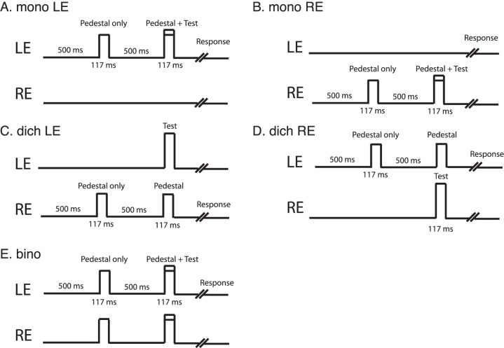
We used the method of Meese et al. (2006) to measure contrast discrimination, except that there was no central fixation point, and a black horizontal line was attached to our stimuli (Figure 1, bottom panel) when both pedestal and test contrasts were in the same eyes (monocular contrast discrimination, Figure 2A, B), in different eyes (dichoptic contrast discrimination, Figure 2C, D), and in both eyes (binocular contrast discrimination, Figure 2E). The procedure was similar to that of the contrast-matching experiment. The observer's task was to judge which interval contained the test (higher contrast). At each pedestal contrast, five one-up-three-down staircases were interleaved to measure two monocular, two dichoptic, and one binocular contrast-discrimination threshold (blocked in one session).
Figure 2.
Procedure for contrast-discrimination task. (A–B) Monocular contrast discrimination: Both the pedestal and test are in the same eye; its threshold was defined as the average of the two eyes' monocular contrast-discrimination threshold (= monoLE/2 + monoRE/2). (C and D) Dichoptic contrast discrimination: The pedestal and test are in different eyes; its threshold was defined as the average of the two eyes' dichoptic contrast-discrimination threshold (= dichLE/2 + dichRE/2). Binocular contrast discrimination was measured with the pedestal and test in both eyes. For control experiments with a central fixation point, the fixation point was continually presented to the two eyes during the whole trial for 500 + 117 + 500 + 117 ms.
Control experiments: The role of the fixation point
Because we found an unexpected binocular advantage in contrast discrimination at a high contrast level, we conducted three control experiments for monocular and binocular contrast discrimination when the pedestal (or standard) contrast was 0.48 and a central fixation point (FP) was present or absent. In all three control experiments, the FP was a white square of 5.3 × 5.3 arcmin. For each trial, following the key press a screen with only the surrounding high-contrast frame, the reference horizontal lines, and the FP was presented to both eyes for 500 ms, followed by sine-wave gratings plus the FP, the reference lines, and the surrounding frame presented to the two eyes for 117 ms. For the first and second control experiments with two internals, the FP, the reference lines, and the surrounding frame continued to be presented to the two eyes until the end of the second interval. The first control experiment was identical to our main contrast-discrimination experiment.
In the second control experiment, we used the method of constant stimuli to measure psychometric functions for contrast discrimination at a pedestal contrast of 0.48. The stimuli were identical to those used in the main experiments, as shown in Figure 1. Each trial contained two intervals, one with a test contrast and one with a standard contrast (0.48). The observer's task was to judge which interval had a higher contrast.
In the third control experiment we used a rating-scale method of constant stimuli. On each trial, the stimulus was presented in only a single interval. The stimulus was a sine-wave grating, identical to that in Figure 1, whose contrast was randomly selected from five contrast levels (0.38, 0.43, 0.48, 0.53, and 0.58). It was presented in either monocular or binocular view with or without an FP. The observer was asked to rate its apparent contrast from lowest (score = 1) to highest (score = 5).
Observers
Four observers with normal or corrected-to-normal vision participated in all three main experiments. The data were averaged across the four observers. Two of the four, plus three additional observers, participated in the control experiments (see Discussion). All observers signed the written consent forms.
Modeling
SDT model for 2AFC contrast discrimination
In SDT, it is assumed that each input contrast evokes an internal response that varies across trials according to a Gaussian distribution. Let m1 and m2 be the contrast of a pair of stimuli, R1 and R2 their internal responses, and σ1 and σ2 the corresponding standard deviations. Using the cumulative Gaussian distribution
 |
the percentage of correct discriminations of the two contrasts is given by
 |
If the initial internal response is fixed—e.g., R1 = 0 and σ1 = 1—Equation 1 still has two unknown parameters, R2 and σ2. With only one measurement P, the solution of Equation 1 is highly ambiguous; multiple solutions exist. Even with multiple pairs of contrasts, the singularity still exists when fitting Equation 1 to the data, making the two mechanisms of NCT and MN inseparable (Katkov et al., 2006). To eliminate the ambiguity in the solution of Equation 1, one more measurement is needed. If we have a robust binocular combination model whose parameters are already known from different binocular tasks, the binocular responses can be deduced from monocular responses, therefore adding one more measurement without additional unknown parameters. Let R and σ2 be the monocular mean response and variance to stimulus m; its binocular mean response and variance are given by R̂(R) and σ̂2(R,σ2), where R̂ and σ̂2 can be deduced from the binocular combination model. For a pair of stimuli m1 and m2, we have another measurement, percentage of correct binocular discriminations:
 |
With two independent equations (Equations 1 and 2), the two unknown parameters can be solved uniquely, providing an opportunity to separate the possible roles of NCT and MN mechanisms in 2AFC contrast discrimination.
Contrast-discrimination mechanisms
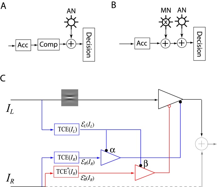
Figure 3A and B shows two different putative contrast-discrimination mechanisms:
Figure 3.
(A) Contrast-discrimination mechanism: NCT or CGC. The contrast signal first goes through both Acc and Comp nonlinearities, and then AN (independent of the input) is added to the signal before the decision. (B) Contrast-discrimination mechanism: MN. The signal first goes through an Acc nonlinearity and then both MN (dependent of the input) and AN (independent of the input) are added to the signal before the decision. (C) Binocular combination model: DSKL model (Ding et al., 2013b). The input to the LE (IL) is first filtered by a narrowband spatial filter at one orientation (here horizontal) and then receives both gain control (blue) and gain enhancement (red) from the RE. The RE-to-LE gain control (blue) and gain enhancement (red) themselves receive gain control from the LE in different gain-control efficiencies α and β, respectively (the gain-control efficiency in the signal path is assumed to be one). For clarity, only the half model for the LE's output is show. The other half for the RE's output has a symmetric structure. The binocular output is linear summation of the two eyes' outputs.
The signal goes through both accelerating (Acc) and compressive (Comp) nonlinearities, and the noise is assumed to be a constant Gaussian additive noise (AN), which is independent of the input. We refer this as the NCT mechanism (Figure 3A).
The signal first goes through an Acc nonlinearity, and both MN (dependent on the input) and AN (independent of the input) are added to the signal. We refer this as the MN mechanism (Figure 3B).
For the NCT mechanism (Figure 3A), the internal response to stimulus m is given by
 |
with constant variance σ2 of Gaussian noise. Equation 3 is identical to the binocular contrast-gain control (CGC), the second stage of the two-stage model (Meese et al., 2006); it is accelerating when m < Z and compressive when m > Z. For the MN mechanism, the internal response is given by
 |
with contrast-dependent variance
 |
of MN and constant variance σ2 of AN. When m < Z, Equation 4 is an Acc contrast transducer, accounting for the “dipper” in the threshold-versus-contrast (TVC) function. When m > Z, it becomes a linear contrast transducer, and the compression is accounted for by MN.
Binocular combination model: DSKL model
Figure 3C shows the half DSKL model for the LE's output (the right eye's [RE's] part in the full model is symmetric to the LE's in normal vision). In the DSKL model, there are three layers for each eye: (a) the selective signal layer (black) that receives both gain control (filled circle) and gain enhancement (open circle) from the other eye and outputs the signal to the binocular summation site; (b) the nonselective gain-control layer (blue) that first extracts and sums image contrast energy (ℰ) across frequency channels and orientations (total contrast energy) and then exerts gain control to the other eye's three layers separately with different gain-control efficiencies (1, α, and β); and (c) the gain-enhancement layer that extracts image contrast energy (ℰ*) and exerts gain enhancement only to the other eye's signal layer. As shown in Figure 3C, before output the LE's signal (black) receives gain control from the RE's gain-control layer (blue), which itself receives gain control from the LE, and also the LE's signal (black) receives gain enhancement from the RE's gain-enhancement layer (red), which receives gain control from the LE. The model output is given by
 |
When two sine-wave gratings with contrast mL and mR are presented to the two eyes, the image contrast energy for gain control is given by
 |
and the image contrast energy for gain enhancement is given by
 |
where gc is the contrast gain-control threshold and ge is the contrast gain-enhancement threshold.
Combination of DSKL model with a contrast-discrimination mechanism
Combined with a binocular combination model (e.g., the DSKL model shown in Figure 3C), a contrast-discrimination mechanism should be able to account for binocular contrast discrimination. Figure 4 shows four different model configurations, inserting either an NCT mechanism (Figure 4A) or an MN mechanism (Figure 4B through D) into the DSKL model. If an NCT (Acc+Comp) is inserted after the binocular combination site (Figure 4A), it should have no effect on the binocular combination—i.e., the modeling results of the DSKL model would remain untouched. However, an NCT before the binocular combination site would distort the binocular combination of the DSKL model, which would violate the linear binocular combination at low contrast levels (Ding et al., 2013b; Ding & Sperling, 2007). Statistically, inserting noise into different loci should have no effect on binocular combination (e.g., perceived phase and contrast of a cyclopean sine wave). Therefore, we tested three model configurations of DSKL+MN by inserting MN into different loci: (a) late MN, after the binocular combination site (Figure 4B); (b) middle MN, before the binocular combination site but after the interocular interaction of the DSKL model (Figure 4C); and (c) early MN, before the DSKL model (Figure 4D). The three model configurations (Figure 4B through D) should have identical performance for monocular contrast discrimination because, when one eye is closed, the DSKL model's output is identical to its input (Ding et al., 2013b). However, for binocular viewing their performance in contrast discrimination would be different, because the signal and noise follow different rules for mathematical operations (e.g., summation, multiplication, and division).
Figure 4.
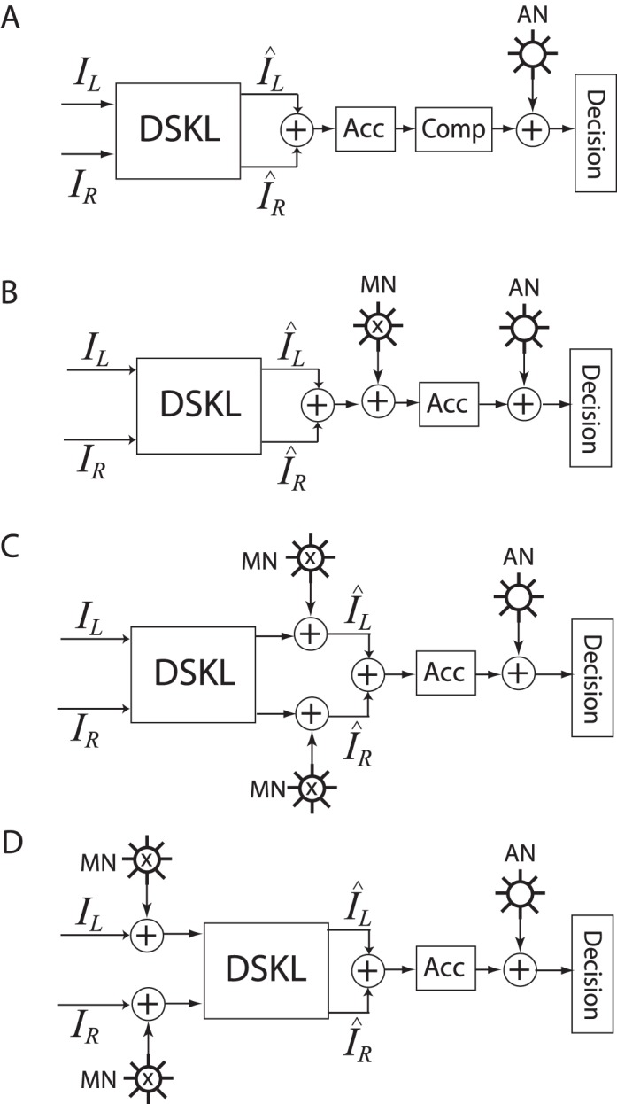
Combination of a binocular combination model (the DSKL model) with NCT (A) or MN (B–D) contrast-discrimination mechanisms. Through inserting MN in different locations, three model configurations for the DSKL+MN combined model are obtained: late-noise model (B), inserting MN after the binocular combination site; middle-noise model (C), inserting MN before the binocular combination site but after the interocular interactions of the DSKL model; and early-noise model (D), inserting MN before the DSKL model.
Results
Monocular contrast discrimination
Figure 5 shows the TVC dipper function for monocular contrast discrimination. When the pedestal contrast is less than the detection threshold, discrimination performance improves (the threshold decreases) with increasing pedestal contrast. This threshold decrease could be explained by an Acc contrast transducer. When the pedestal contrast is greater than the detection threshold, the discrimination performance deteriorates (threshold increases) with increasing pedestal contrast, which may be explained by a Comp contrast transducer or by MN. In the NCT mechanism (Figure 3A), the CGC (Equation 3) includes both Acc and Comp contrast transducers. With the assumption of AN (independent of input), the NCT mechanism (CGC) provides a good fit to the monocular TVC data (the red solid curve in Figure 5). The CGC has four model parameters (p, q, Z, and σ), of which Z reflects the contrast-detection threshold; it would be an Acc contrast transducer when contrast < Z and a Comp contrast transducer when contrast > Z.
Figure 5.
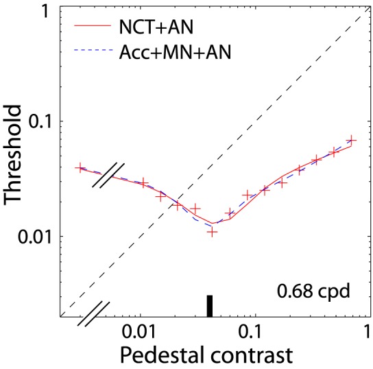
Monocular contrast discrimination (the average of the two eyes of four observers) as a function of pedestal contrast (TVC function). The data were fitted by an NCT plus AN (red curve, see Figure 3A) or by an Acc contrast transducer plus MN plus AN (dashed blue curve, see Figure 3B). The detection threshold (≈ 0.04) is indicated by a short vertical bar in the horizontal axis.
If the Comp contrast transducer is replaced with MN (dependent on the input), the model of an Acc contrast transducer (Equation 4) plus MN (Equation 5; Acc+MN) is also able to account for the monocular contrast discrimination very well (blue dashed curve in Figure 5). When contrast < Z, Equation 4 is an Acc contrast transducer, accounting for the dipper in the TVC function. When contrast > Z, Equation 4 becomes a linear contrast transducer and the compression is accounted for by MN (Equation 5).
Table 1 shows the best-fitting parameters of the NCT (CGC) and MN mechanisms and their chi-square values. Both the NCT and MN provide reasonable fits to the monocular contrast-discrimination data. Is it possible to obtain a better fit using both a Comp contrast transducer and MN to account for the compression mechanism? As shown in Table 1, adding a Comp contrast transducer to MN (CGC+MN) has no benefit in the model fit. The fitting curve (not shown) of CGC+MN is very similar to that of Acc+MN. This result—i.e., that NCT and MN are indistinguishable in their ability to fit monocular data (see Figure 5)—is the issue we are faced with, and which we introduced earlier.
Table 1.
Model parameters for monocular contrast discrimination and their fitting chi-squares. Notes: Np: Number of parameters. ν: Number of degrees of freedom. CGC: Contrast-gain control. Acc: Accelerating nonlinearity. MN: Multiplicative noise.
Perceived phase and contrast of a cyclopean sine wave: Testing the DSKL model
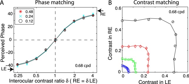
Figure 6 shows the perceived phase (A) and contrast (B) of a cyclopean sine wave, for different interocular contrast ratios. The data were averaged across the two eyes to remove any possible binocular bias, and averaged across the four observers. We used one set of model parameters (Table 2) to fit both the phase and contrast data sets to the DSKL model (smooth curves in Figure 6). The reduced chi-square for model fitting is 2.44.
Figure 6.
(A) Results of the phase-matching experiment: the perceived phase of a cyclopean sine wave as a function of interocular contrast ratio. (B) Results of the contrast-matching experiment: the binocular equal-contrast contour when standard contrast was 0.48, 0.24, 0.12, and 0.06. The data were averaged across the two eyes to remove any possible binocular bias, and averaged across four observers. The solid lines in (A) and (B) are the best fits of the DSKL model (Table 2 shows its best-fitting parameters).
Table 2.
Parameters of the DSKL model. Note: The reduced chi-square  = 2.44.
Binocular contrast discrimination: Testing a late contrast-discrimination mechanism
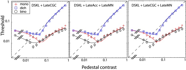
Combined with the DSKL model, a contrast-discrimination mechanism should be able to account for three data sets—monocular, dichoptic, and binocular contrast discrimination—with one set of model parameters. In combination with the DSKL model whose parameters are given in Table 2, we fit a late contrast-discrimination mechanism (CGC, MN, or CGC+MN) to the three contrast-discrimination data sets (Figure 7). However, adding dichoptic and binocular contrast discrimination at each pedestal was not helpful in distinguishing among the late contrast-discrimination mechanisms (Table 3). Because in a late contrast-discrimination mechanism both the signal and noise are calculated from the binocular combined contrast, the two extra measurements are just two extra data points from the same mechanism. In other words, Equations 1 and 2 are not independent for a late contrast-discrimination mechanism; the ambiguity in solution still exists. It is easy to show that when the internal responses (or perceived contrast) are the same in monocular (Equation 1) and binocular (Equation 2) conditions, their discrimination performance would also be the same.
Figure 7.
A contrast-discrimination mechanism—late CGC, late Acc+MN, or late CGC+MN—in combination with the DSKL model, was fitted to the monocular, dichoptic, and binocular contrast-discrimination data. The parameters for the DSKL model are given in Table 2.
Table 3.
Model parameters for monocular, dichoptic, and binocular contrast discrimination and their fitting chi-squares. Notes: Np: Number of parameters. ν: Number of degrees of freedom. CGC: Contrast-gain control. Acc: Accelerating nonlinearity. MN: Multiplicative noise.
Predictions of binocular contrast discrimination: Where to insert MN?
If the MN is inserted before the binocular combination site, Equation 2 might become independent of Equation 1. Because the signal and noise follow different summation rules, Equation 2 might provide different information that cannot be deduced from Equation 1; contrary to the scenario considered in the previous paragraph, when the internal responses are the same in monocular (Equation 1) and binocular (Equation 2) conditions the discrimination performances are different.
However, it is very hard to fit the combined model with early MN, because the analytic formula for the variance of the binocular combined noise is not available. Here we used a different strategy to test where to insert MN. With the parameters of the DSKL model (Table 2) and a contrast mechanism (Table 1), we were able to test whether their combinations, shown in Figure 4, can predict binocular and dichoptic contrast discrimination without any model fitting. With the NCT inserted after the binocular combination site in the DSKL model (DSKL plus late NCT, Figure 8A), the combined model predicts binocular and dichoptic contrast discrimination quite well (reduced chi-square for prediction:  = 9.77; solid curves in Figure 8A); it captures the main features of TVC functions for binocular and dichoptic contrast discrimination. However, the prediction systematically overestimates the discrimination thresholds of almost all data points in the compressive handle; the internal noise in binocular contrast discrimination seems to be lower than that in monocular contrast discrimination. Inserting the NCT before the binocular combination site (early NCT) distorts the model predictions for perceived phase and contrast, and refitting the combined model (DSKL plus early NCT) to the three data sets (perceived phase, perceived contrast, and contrast discrimination) was also unsuccessful.
Figure 8.
Predictions for binocular and dichoptic contrast discrimination by the DSKL model plus a contrast-discrimination mechanism. The parameters of the DSKL model are obtained from fitting it to the perceived-phase and perceived-contrast data (see Figure 6 and Table 2), and the parameters of a contrast-discrimination mechanism (either NCT or MN) are obtained from fitting it to the monocular contrast-discrimination data (see Figure 5 and Table 1). The dichoptic contrast-discrimination data were averaged between the two eyes. (A) Predictions of the DSKL model plus late NCT. (B) Predictions of the DSKL model plus late MN. (C) Predictions of the DSKL model plus middle MN. (D) Predictions of the DSKL model plus early MN. The predictions of the DSKL model plus middle or early NCT are not shown because they are very poor, even out of range of the plot. The monocular data and model fits are also shown (dashed red curve).
Please note that in the MN mechanism, the monocular TVC function was fitted with the MN inserted after the Acc. In order to predict discrimination data when inserting MN in different loci, we moved the MN before the Acc, which slightly increased the monocular discrimination threshold (solid red line in Figure 8B through D) around m ≈ Z (the shallowest point) with little effect on the other thresholds. At low contrast (when m < Z), MN is too small and the AN dominates performance, while at high contrast (when m > Z), the Acc (Equation 4) becomes a linear contrast transducer. Similar to the combined model with late NCT (Figure 8A), the combined model with late MN overestimates binocular discrimination thresholds at high contrast (Figure 8B), although it captures the main features of the TVC functions ( = 14.26). Moving MN before the binocular combination site but after interocular interactions (middle MN, Figure 8C) improves the prediction (
 = 12.11), and further moving MN before interocular interactions (early MN, Figure 8D) makes the prediction nearly perfect (
 = 4.82).
Discussion
We have compared two putative contrast-discrimination mechanisms, NCT and MN, by combining them with the DSKL binocular combination model. We found that inserting early MN in the combined model provides the best account of binocular contrast discrimination. Is this conclusion a consequence of the DSKL model, or do other binocular combination models give similar results? To answer this question, we compared the DSKL, Ding–Sperling, and two-stage models by combining them with either NCT or MN to explain binocular contrast discrimination.
From our previous studies (Ding et al., 2013b; Ding & Sperling, 2006), the output of the Ding–Sperling model is given by
 |
which contains no interocular enhancement when compared with the DSKL model (Equation 6). The two-stage model was originally proposed to account for monocular, dichoptic, half-binocular, and binocular contrast discrimination (Meese et al., 2006), and was later used to account for the perceived contrast of a cyclopean sine wave (Baker et al., 2007). Recently, the model has been developed to account for a total of 11 different types of dipper function with various combinations of pedestal, increments, and decrements for targets (Georgeson, personal communication). In our previous study (Ding et al., 2013b), we extended it to explain binocular phase combination by assuming that the operation in the signal path has no effect on the phase. The output of the first stage of the two-stage model is given by
 |
where the exponent operation is assumed to act only on the contrast, without any effect on the phase. The second stage of the two-stage model is identical to the NCT mechanism (Equation 3), the binocular CGC.
Although Equations 9 and 10 are similar, the first stage of the two-stage model (Equation 10) contains both monocular and interocular CGCs, while the Ding–Sperling (Equation 9) and DSKL models (Equation 5) contain only interocular CGCs (double layered). With monocular CGC, the first stage of the two-stage model also affects monocular contrast perception, which distorts the monocular contrast discrimination in the combined model—i.e., the monocular performance in contrast discrimination depends on where the MN is inserted. Like the DSKL model, the Ding–Sperling model has no effect on monocular contrast perception; inserting MN in different loci has no effect on monocular contrast discrimination. After simulation, we found that, similar to the DSKL model, the best model configuration is the one with early MN inserted before the Ding–Sperling model (data not shown).
In the following, we first compare these models in fitting the perceived phase and contrast of cyclopean sine waves to obtain their best fits for binocular combination; then in combination with either a late NCT or a late MN contrast-discrimination mechanism, we compare them in fitting the late NCT or late MN to monocular, dichoptic, and binocular contrast-discrimination data.
Model comparison in fitting the perceived phase and contrast of cyclopean sine waves
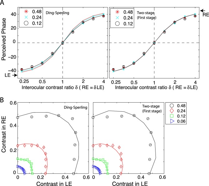
Figure 9 shows the best fits of the Ding–Sperling and two-stage models to both phase (Figure 9A) and contrast data (Figure 9B). For the two-stage model, only the first stage was used to account for binocular phase and contrast combination. Consistent with our previous study (Ding et al., 2013b), with constraints of perceived phase the two models provide a poor fit to the perceived-contrast data at higher contrast levels. After the addition of interocular enhancement to the Ding–Sperling model, the DSKL model is able to explain both the linear summation at lower contrast levels and the winner-take-all summation at higher contrast levels (Figure 6). Table 4 shows the best fits and fitting statistics of the three models.
Figure 9.
Model comparison in fitting the perceived phase and contrast of cyclopean sine waves.
Table 4.
Model parameters for fitting perceived-phase and perceived-contrast and model-fitting statistics. Notes: Np: Number of parameters. ν: Number of degrees of freedom.
Model comparison in explaining binocular contrast discrimination
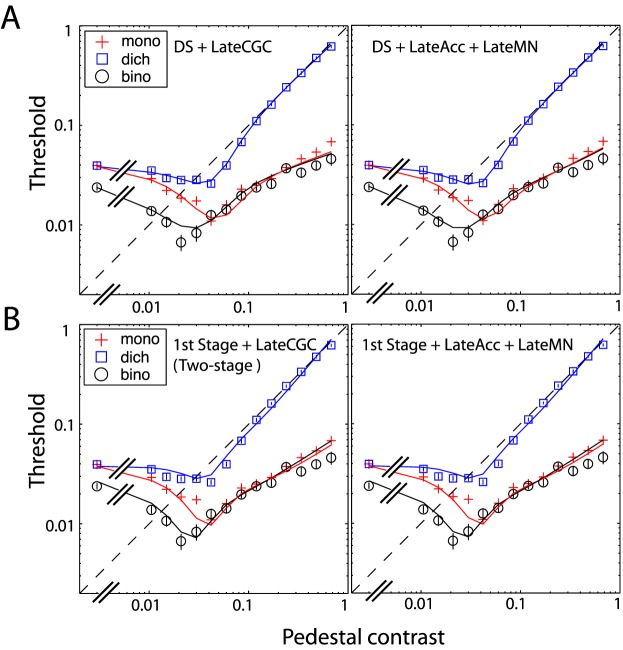
How well do these binocular combination models account for binocular contrast discrimination? To answer this question, we fitted the late NCT and late MN mechanisms, combined with one of these models, to the monocular, dichoptic, and binocular contrast-discrimination data. The parameters of these binocular combination models are given in Table 4; Figure 10 shows the comparison. A late contrast-discrimination mechanism combined with the Ding–Sperling model provides a better fit than when combined with the first stage of the two-stage model or with the DSKL model. However, considering the combined model in explaining perceived phase, perceived contrast, and contrast discrimination, the DSKL+lateNCT and DSKL+lateMN perform best (Table 5). Consistent with the combined model with the DSKL model, combined with the Ding–Sperling model or the first stage of the two-stage model, the late NCT and late MN cannot be distinguished in the 2AFC contrast-discrimination task.
Figure 10.
Fitting late NCT (left column) and late MN (right column)—attached to the Ding–Sperling model (A) or the first stage of the two-stage model (B)—to three data sets of monocular, dichoptic, and binocular contrast discrimination. The parameters of the Ding–Sperling model and the first stage of the two-stage model are obtained by fitting them to the binocular combined phase and contrast, which are given in Table 4.
Table 5.
Model-fitting statistics. Notes: Np: Number of parameters. ν: Number of degrees of freedom. MN: Multiplicative noise. DS: Ding–Sperling. NCT: Nonlinear contrast transducer. The right column shows fitting statistics for late NCT or late MN when attached to a binocular combination model. The left column shows fitting statistics for a combined model (a binocular combination model fitting to perceived phase and contrast—Table 4—plus the contrast-discrimination model fitting to contrast-discrimination data).
Model simulation of internal noise
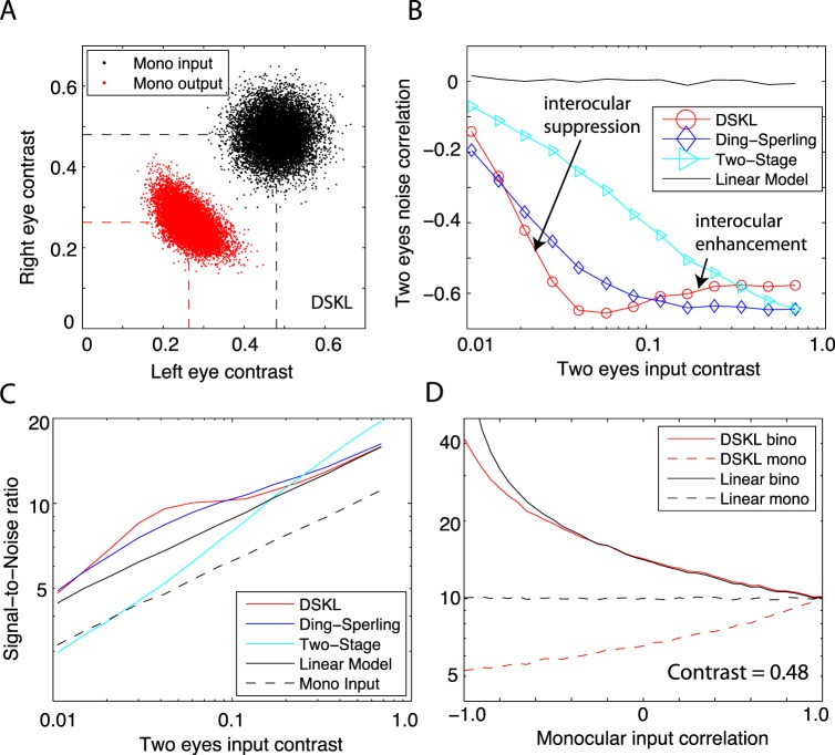
Inserting MN before the summation site (middle or early MN) increases the signal-to-noise ratio because, after summation, the signal would be doubled while the noise increases by only  . To further understand the properties of a binocular combination model, we simulated the model with early noise added to the input of the model. Figure 11 shows the simulation results when the two eyes are presented with identical mean contrast m with an early Gaussian MN—i.e., LE = m + 𝒩L(0,σm) and RE = m + 𝒩R(0,σm), where σm = kma (k = 0.08, a = 0.70, from Table 1). The model was simulated without considering the NCT and AN after the binocular combination site. For the two-stage model (parameters from Table 4), we simulated only the first stage.
Figure 11.
Model simulation of early monocular MN added before binocular combination. (A) Joint distributions of two monocular inputs (black) and two monocular outputs (red) of the DSKL model. The two eyes' inputs are LE = 0.48 + 𝒩L(0,σ) and RE = 0.48 + 𝒩R(0,σ), with identical mean contrast plus independent Gaussian noise (black dots, correlation = 0). The dashed black lines indicate the mean values of the two eyes' inputs, and the dashed red lines indicate the mean values of the two outputs. Ten thousand trials were simulated. (B) The correlations of model monocular outputs when the two eyes are presented with identical mean contrast with early multiplicative Gaussian noise (input correlation = 0). For the two-stage model, only the first stage was used in the simulation. (C) Signal-to-noise ratio of the binocular output of a model as a function of monocular-input contrast. The monocular-input signal-to-noise ratio is also indicated (black dashed line). (D) Binocular signal-to-noise ratio of the DSKL model (red) and the linear-summation model (black) as a function of monocular-input correlation with mean input contrast = 0.48. The signal-to-noise ratios of model monocular outputs are indicated in red (DSKL) and black (linear model) dashed curves.
When the monocular mean contrast is 0.48 and two independent Gaussian noise sources are added to the two eyes, the joint distribution of the two inputs is spherical (black points in Figure 11A). However, the joint distribution of the two monocular outputs of the DSKL model (parameters from Table 2) is an ellipse whose long axis lies along the antidiagonal showing an anticorrelated relationship of the two monocular outputs (red points in Figure 11A). Any binocular combination model with interocular suppression would have anticorrelated monocular outputs if independent noise were added to each of its inputs. Figure 11B shows the correlation of model monocular outputs when the two eyes' mean contrast varies and their noise is uncorrelated. For models with interocular suppression, such as the first stage of the two-stage model, the Ding–Sperling model (parameters from Table 4), and the DSKL model, the anticorrelation of the model monocular outputs increases when the input mean contrast increases. The correlation of the DSKL monocular outputs initially decreases rapidly, and after reaching the minimum point, it increases slowly because of interocular enhancement. In contrast, for models without interocular enhancement—such as the two-stage model and the Ding–Sperling model— monocular-output correlation decreases monotonically.
Does mutual suppression increase the binocular signal-to-noise ratio because it results in anticorrelated monocular outputs? To answer this question, we simulated the signal-to-noise ratio of the binocular output of a model when its mean input contrast varied. As shown in Figure 11C, for the first stage of the two-stage model the binocular signal-to-noise ratio is similar to the monocular input at low contrast levels, and increases as input contrast increases, even beyond that of the linear-summation model at high contrast levels. For the Ding–Sperling and DSKL models, the signal-to-noise ratios are higher than that of the linear-summation model at all contrast levels.
The simulations described are based on independent noise in the two eyes (correlation = 0). However, early noise in the two eyes may not be completely independent. For example, if fluctuations in accommodation and/or fixational eye movements are the noise sources, the noise in the two eyes might be correlated (Campbell, 1960; Charman & Heron, 1988, 2015; Heron, Winn, Pugh, & Eadie, 1989). Figure 11D shows the simulation results when the correlation of the two monocular inputs varies. At a mean contrast of 0.48, the binocular signal-to-noise ratio of the DSKL model decreases when the correlation increases, almost parallel to that of the linear-summation model, while the signal-to-noise ratio of the monocular input remains constant. The nonlinear operations in the model decrease the signal-to-noise ratio of its monocular outputs (dashed red curves), counteracting the anticorrelation effect and resulting in the binocular output having a comparable signal-to-noise ratio to the linear-summation model at higher contrast levels. At lower contrast levels, the operations become more linear, resulting in less decrease of the monocular signal-to-noise ratio but also less anticorrelation of the two monocular outputs. In the end, the binocular signal-to-noise ratios of the DSKL and Ding–Sperling models are almost parallel to that of the linear-summation model at both higher and lower ends of input contrast. At middle contrast levels, however, the performance of the DSKL and Ding–Sperling models is much better (higher binocular signal-to-noise ratio) than predicted by linear summation (Figure 11C).
Early versus late noises
It is obvious that, in the visual system, each stage produces internal noise. However, the gains of each stage are sufficient to amplify the unavoidable noise of the first stage (i.e., photon noise) so that it dwarfs the additional noise that arises at later stages (Pelli, 1991). One can always reduce the effect of the late noise by increasing the gain of earlier amplifiers. For well-designed systems, including the human visual system that has evolved over millions of years, it would be reasonable to assume that early noise might be the main limitation. Although Pelli (1991) argues that psychophysical models of the visual system should incorporate noise at the first stage, rather than injecting an arbitrary noise later, many models use late noise to interpret their results because it is more difficult to analyze a nonlinear system with early noise. In this study, we also placed constant AN (independent of input) in the last stage, but we cannot exclude the possibility that this late constant noise might have an early source—e.g., the inevitable fluctuations in the number of quanta absorbed in the retina, which depends on the background luminance (De Vries, 1943; Rose, 1942, 1948). For constant noise, it is not a large issue to insert it in different loci, but for MN (dependent on input), as shown in this study, the system performance is dependent on its location.
Binocular advantage
It is clear that at low contrasts, viewing with two eyes is better than with one. For contrast-detection tasks, Legge (1984a) reported that the binocular threshold was ∼1.5 times lower than the monocular threshold, and Meese et al. (2006) showed that the binocular summation ratio was ∼1.6. In this study, we found that the binocular summation ratio for contrast detection (contrast discrimination when pedestal = 0) was ∼1.65 averaged across four observers. In an extensive modeling study on detection threshold, Meese and Summers (2009) tested 62 different models to predict both binocular summation and area summation. For detection thresholds, they found that the best model was linear summation across eyes, followed by an Acc contrast transducer and late Gaussian noise. In this study, however, we tested models over a wide range of contrasts, and they can be further reduced to their simplified forms at the detection threshold. Actually, at the detection-threshold level, the DSKL model can be reduced to a linear-summation model, the NCT can be reduced to an Acc contrast transducer, and MN can be ignored because late AN dominates the system. Therefore, all four model architectures (Figure 4) tested in this study can be reduced to be the best model of Meese and Summers (2009) for binocular summation at the detection threshold.
For contrast-discrimination tasks, binocular performance is also much better than monocular performance at low contrast levels. However, it is unclear whether there is a binocular advantage in contrast discrimination at high contrast levels. In this study, we found a binocular advantage when the contrast was below 3% or above ∼34%. However, in the middle range from ∼4% to 30%, binocular performance is similar to monocular performance. With binocular CGC (late NCT) followed by Gaussian AN, all three binocular combination models (two-stage, Ding–Sperling, and DSKL) predict similar contrast-discrimination performance in binocular and monocular viewing at higher contrast levels. Only by inserting MN in the early stage of binocular vision can a binocular model with mutual suppression predict a binocular advantage at high contrast. Therefore, the question of whether there is a binocular advantage at high contrast levels may provide the decisive test of whether the binocular system needs early monocular MN. However, previous studies (Baker, Meese, & Hess, 2008; Legge, 1984b; Maehara & Goryo, 2005; Meese et al., 2006) have not reported a binocular advantage in contrast discrimination at high contrast levels. One reason might be that the pedestal contrast in previous studies was not high enough. For example, the highest pedestal contrast in previous studies was just 31.6%, at which a small binocular advantage was displayed by both observers in the study by Legge (1984b) but not by those in the work by Meese et al. (2006) and Baker et al. (2008). Similar to these studies, we find no binocular advantage for contrasts between about 4% and 30%.
Effects of fixation points
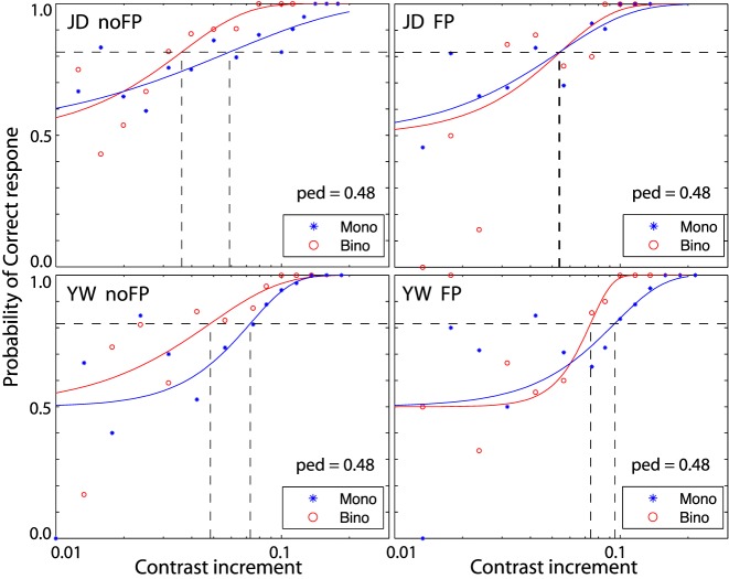
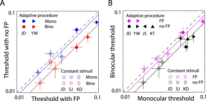
One potentially important difference between our study and those of others is the absence of a central FP in the current study. The use of FPs in visual psychophysics is common practice (Summers & Meese, 2009). To study any possible effects of FPs, we performed three control experiments. In the first control experiment, we used the same adaptive procedure as in our main experiment to measure contrast discrimination (pedestal contrast = 48%) in two of our four observers with and without central FPs (Figure 12). As noted in Methods, the FP was a single point in the center of the display seen by both eyes. For both observers, the main effect of the FP was to substantially elevate binocular thresholds while having much less effect on monocular thresholds. Thus, the binocular advantage was more evident when the FP was absent than when it was present. This may be another reason why the binocular advantage was not noticed in previous studies. For observer JD, with a central FP the binocular contrast-discrimination threshold (0.054 ± 0.009) was very similar to the monocular one (0.054 ± 0.009). However, with no FP the binocular contrast-discrimination threshold (0.036 ± 0.005) was better than the monocular one (0.059 ± 0.008). Observer YW showed a slight binocular advantage even with a central FP (binocular threshold: 0.074 ± 0.009; monocular: 0.095 ± 0.013), and the binocular advantage increased (binocular threshold: 0.048 ± 0.007; monocular: 0.073 ± 0.006) without it.
Figure 12.
Psychometric functions of monocular and binocular contrast discrimination at a pedestal of 48% when a central FP was present (left) or absent (right). A one-up-three-down adaptive procedure was used. The data were fitted with a Weibull function (Meese et al., 2006). At the threshold, the discrimination performance is 81.6%.
In the second control experiment, we used the method of constant stimuli to measure contrast discrimination with a pedestal contrast of 48% when a FP was present or absent. Figure 13 shows the probability of reporting the test contrast higher than the standard contrast (48%) as a function of test contrast. The data were fitted with a Weibull function. The point of subjective equality at 50% probability should be equal to the standard contrast (48%). The slope of the curve reflects the contrast-discrimination threshold (corresponding to 75% correct), and it also reflects the internal noise (steeper meaning less internal noise). Because the results were dependent on whether the test was in the first interval (Figure 13, left column) or in the second interval (Figure 13, right column), we averaged the results across the orders. We tested three observers. Observer JD was one of four who participated in our main experiments, and the other two observers participated in only the control experiments. Without a central FP (Figure 13A), for observers JD and KD the binocular advantage could be observed (less internal noise under binocular view) whether the test was in the first or the second interval. However, for observer SJ the binocular threshold was much lower than the monocular when the test was in the first interval, while it was slightly higher when the test was in the second interval. On average, for observer SJ the binocular advantage was still evident (less internal noise under binocular view) when the FP was absent. When the central FP was present (Figure 13B), the binocular advantage was less evident for all three observers.
Figure 13.
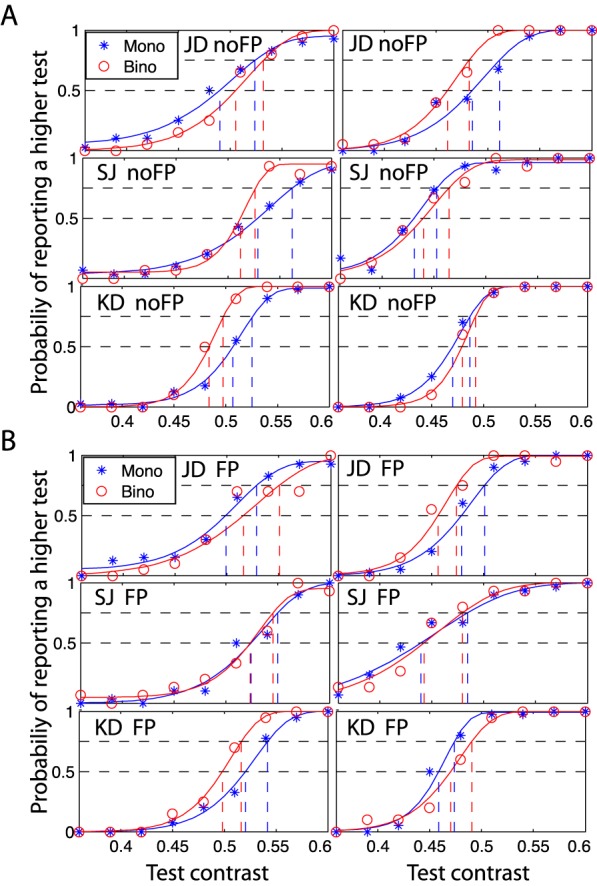
Psychometric functions: probability of reporting that the test grating has higher contrast than the standard as a function of test contrast. The method of constant stimuli was used to match a test contrast (= 0.38 ∼ 0.6) to the standard (= 0.48), presented in the two consecutive intervals, when a central FP was absent (A) or present (B). The test contrast was in either the first interval (left) or the second (right).
Figure 14 summarizes the FP effects (A) and binocular advantage (B) in contrast discrimination using both the adaptive procedure and the method of constant stimuli when the standard contrast was 48%. We did a bootstrap analysis on the psychometric functions (Figures 12 and 13) to estimate error bars, p values, and confidence intervals. Consistent with a previous study (Summers & Meese, 2009), the FP had no significant masking effect on monocular contrast discrimination (Figure 14A). Averaged across observers, the masking effect on monocular contrast discrimination was only a factor of 1.10 (95% CI [0.94, 1.29], p = 0.115). However, under binocular viewing, contrast discrimination was significantly improved when the FP was absent. This phenomenon has not been reported previously and cannot be simply explained by the FP's masking effect. Averaged across observers, the improvement in binocular contrast discrimination with no FP was a factor of 1.45 (95% CI [1.19, 1.91], p = 0.025).
Figure 14.
(A) Comparison of contrast-discrimination threshold when a central FP was absent versus present. (B) Comparison of binocular versus monocular contrast-discrimination threshold. The pedestal (or standard) contrast was 48%. Error bar indicates the standard errors estimated from the bootstrap analysis of psychometric functions.
Figure 14B shows the binocular advantage when the FP was absent (black) and present (magenta). Consistent with previous studies (Baker et al., 2008; Legge, 1984b; Maehara & Goryo, 2005; Meese et al., 2006), when the FP was present there was no significant advantage of binocular over monocular viewing in contrast discrimination. Averaged across observers, when the FP was present the binocular advantage was only a factor of 1.13 (95% CI [0.89, 1.34], p = 0.21). However, when the FP was absent, binocular contrast discrimination was significantly better than monocular contrast discrimination, a key phenomenon observed in this study which has not been reported previously. Averaged across observers, when the FP was absent the binocular advantage was a factor of 1.39 (95% CI [1.09, 1.60], p = 0.001).
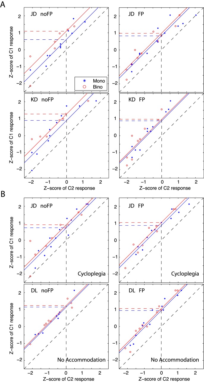
In the third control experiment, observers were asked to rate the contrast presented in a single interval. The z-scores of two consecutive contrast levels (C2 − C1 = 0.05) are compared in Figure 15. An SDT model with linear contrast response and constant noise was used to fit the data (solid lines). Consistent with the previous two control experiments, observers JD and KD showed more binocular advantage when the FP was absent than present (Figure 15A). However, after a cycloplegic (two drops of 1% cyclopentolate) was used to paralyze JD's accommodation, the binocular advantage disappeared (Figure 15B, top panel); binocular contrast-discrimination performance was only slightly better than monocular, whether the FP was present or absent.
Figure 15.
Comparison of C1 versus C2 contrast responses in z-scores (receiver operating characteristic curves). A sine-wave grating with contrast randomly selected from one of five levels (0.38, 0.43, 0.48, 0.52, 0.58) was present in either monocular (blue) or binocular (red) view when a central FP was absent or present. An observer was asked to rate the contrast with five scores from lowest (1) to highest (5). The responses of the two consecutive contrast levels (C2 − C1 = 0.05) were compared in their z-scores. The discrimination d′ is indicated by the z-score of the C1 response when the z-score of C2 response is 0 (the cross point of vertical black dashed line with a receiver operating characteristic curve). (A) Performance of observers with accommodation. (B) Performance of observers without accommodation, because of cycloplegia (JD) or absolute presbyopia (DL).
Our working hypothesis is that in the absence of an FP, fluctuations in accommodation (and thus, accommodative convergence) are larger than when a FP is present, and that these fluctuations are responsible for the binocular advantage (discussed in more detail later). If this hypothesis is correct, a senior observer without accommodation should have no binocular advantage even when a FP is absent. As shown in the bottom panel of Figure 15B, this is exactly what we found. Observer DL—who is in his late 60s and an absolute presbyope and has no accommodation at the 68-cm viewing distance (Wolfe et al., 2015)—showed similar contrast-discrimination performance in monocular and binocular viewing whether the FP was present or absent.
Although it needs to be further studied in the future, fluctuations in accommodation might be one source of early monocular noise that results in a different binocular advantage depending on whether the FP is present or absent. There is a considerable amount of biological noise in the accommodation system (Campbell, Robson, & Westheimer, 1959). Under steady viewing conditions, the refractive power of the human lens fluctuates in time by fractions of a diopter. Campbell (1960) reported that the variations in refractive power were very similar (correlated) in the two eyes when a high-contrast FP was viewed at 50 cm. Heron et al. (1989) also reported that the steady-state accommodation in both eyes was highly correlated. However, under natural viewing conditions it is not clear if accommodation is dynamically correlated between the two eyes. Chin, Hampson, and Mallen (2008) used a binocular Shack–Hartmann wave-front sensor to measure the ocular wave-front aberrations concurrently in both eyes of six observers at a sampling rate of 20.5 Hz. They did coherence function analysis in the frequency domain and found that the dynamic correlation between the aberrations of the two eyes was poor. We speculate that the FP might be helpful in maintaining the steady-state accommodation of the two eyes, resulting in the two eyes' early noise becoming more correlated and thus increasing the binocular noise (Figure 11D) and reducing the binocular advantage (relative to no FP).
Campbell (1960) suggested that the amplitude of accommodation fluctuations could be smaller under binocular conditions, possibly due to the stabilizing effect of the convergence-fixation reflex, which was supported by later studies (Charman & Heron, 2015; Mira-Agudelo, Lundström, & Artal, 2009; Seidel, Gray, & Heron, 2005). We speculate that, in monocular viewing when the stimulus is present in only one eye, the binocular FP might also be helpful in maintaining binocular convergence, resulting in less monocular noise than when the FP is absent and thus reducing the binocular advantage.
Conclusion
The combination of a binocular model with a contrast-discrimination mechanism provides an opportunity to test both the binocular model and the contrast-discrimination mechanism. Our results show that the DSKL model can readily account for three different binocular tasks—binocular combined phase and contrast and binocular contrast discrimination—using a single set of model parameters, and that early monocular multiplicative noise plays an important role in contrast discrimination.
Supplementary Material
Acknowledgments
This work was supported by National Eye Institute grants R01EY01728 and R01EY020976 and a James S. McDonnell Foundation grant—Collaborative Network for Critical Period Re-Examination (Brain CPR). The authors thank Dr. Stanley Klein for useful suggestions, Dr. Mark Georgeson and Dr. Timothy Meese for discussions on the binocular advantage and the fixation-point effect, and Ms. Yuan Wang and Ms. Fiona Yuan for collecting part of the data.
Commercial relationships: none.
Contributor Information
Jian Ding, jian.ding@berkeley.edu, http://levilab.berkeley.edu/.
Dennis M. Levi, dlevi@berkeley.edu, http://levilab.berkeley.edu/.
References
- Baker D. H.,, Meese T. S.,, Georgeson M. A. (2007). Binocular interaction: Contrast matching and contrast discrimination are predicted by the same model. Spatial Vision, 20 (5), 397–413. [DOI] [PubMed] [Google Scholar]
- Baker D. H.,, Meese T. S.,, Hess R. F. (2008). Contrast masking in strabismic amblyopia: Attenuation, noise, interocular suppression and binocular summation. Vision Research, 48 (15), 1625–1640. [DOI] [PubMed] [Google Scholar]
- Baker D. H.,, Wallis S. A.,, Georgeson M. A.,, Meese T. S. (2012). The effect of interocular phase difference on perceived contrast. PLoS One, 7 (4), e34696. [DOI] [PMC free article] [PubMed] [Google Scholar]
- Campbell F. (1960). Correlation of accommodation between the two eyes. Journal of the Optical Society of America, 50 (7), 738–738. [DOI] [PubMed] [Google Scholar]
- Campbell F.,, Robson J.,, Westheimer G. (1959). Fluctuations of accommodation under steady viewing conditions. The Journal of Physiology, 145 (3), 579–594. [DOI] [PMC free article] [PubMed] [Google Scholar]
- Charman W.,, Heron G. (1988). Fluctuations in accommodation: A review. Ophthalmic and Physiological Optics, 8 (2), 153–164. [DOI] [PubMed] [Google Scholar]
- Charman W. N.,, Heron G. (2015). Microfluctuations in accommodation: An update on their characteristics and possible role. Ophthalmic and Physiological Optics, 35 (5), 476–499. [DOI] [PubMed] [Google Scholar]
- Chin S.,, Hampson K.,, Mallen E. (2008). Binocular correlation of ocular aberration dynamics. Optics Express, 16 (19), 14731–14745. [DOI] [PubMed] [Google Scholar]
- De Vries H. (1943). The quantum character of light and its bearing upon threshold of vision, the differential sensitivity and visual acuity of the eye. Physica, 10 (7), 553–564. [Google Scholar]
- Ding J.,, Klein S. A.,, Levi D. M. (2013a). Binocular combination in abnormal binocular vision. Journal of Vision, 13 (2): 14, 1–31, doi:10.1167/13.2.14 [PubMed] [Article] [DOI] [PMC free article] [PubMed] [Google Scholar]
- Ding J.,, Klein S. A.,, Levi D. M. (2013b). Binocular combination of phase and contrast explained by a gain-control and gain-enhancement model. Journal of Vision, 13 (2): 13, 1–37, doi:10.1167/13.2.13 [PubMed] [Article] [DOI] [PMC free article] [PubMed] [Google Scholar]
- Ding J.,, Klein S.,, Levi D. (2013c). Binocular contrast discrimination needs monocular multiplicative noise. Journal of Vision, 13 (9): 550, doi:10.1167/13.9.550 [Abstract] [DOI] [PMC free article] [PubMed] [Google Scholar]
- Ding J.,, Sperling G. (2006). A gain-control theory of binocular combination. Proceedings of the National Academy of Sciences, USA, 103 (4), 1141–1146. [DOI] [PMC free article] [PubMed] [Google Scholar]
- Ding J.,, Sperling G. (2007). Binocular combination: Measurements and a model. Harris L., Jenkin M. (Eds.), Computational vision in neural and machine systems (pp. 257–305). Cambridge, UK: Cambridge University Press. [Google Scholar]
- Georgeson M. A.,, Meese T. S. (2006). Fixed or variable noise in contrast discrimination? The jury's still out…. Vision Research, 46 (25), 4294–4303. [DOI] [PubMed] [Google Scholar]
- Green D. M.,, Swets J. A. (1966). Signal detection theory and psychophysics. New York: Wiley. [Google Scholar]
- Heron G.,, Winn B.,, Pugh J. R.,, Eadie A. S. (1989). Twin channel infrared optometer for recording binocular accommodation. Optometry & Vision Science, 66 (2), 123–129. [DOI] [PubMed] [Google Scholar]
- Huang C. B.,, Zhou J.,, Zhou Y.,, Lu Z. L. (2010). Contrast and phase combination in binocular vision. PLoS One, 5 (12), e15075. [DOI] [PMC free article] [PubMed] [Google Scholar]
- Katkov M.,, Tsodyks M.,, Sagi D. (2006). Singularities in the inverse modeling of 2AFC contrast discrimination data. Vision Research, 46 (1), 259–266. [DOI] [PubMed] [Google Scholar]
- Klein S. A. (2006). Separating transducer non-linearities and multiplicative noise in contrast discrimination. Vision Research, 46 (25), 4279–4293. [DOI] [PubMed] [Google Scholar]
- Kontsevich L. L.,, Chen C. C.,, Tyler C. W. (2002). Separating the effects of response nonlinearity and internal noise psychophysically. Vision Research, 42 (14), 1771–1784. [DOI] [PubMed] [Google Scholar]
- Legge G. E. (1984a). Binocular contrast summation—I. Detection and discrimination. Vision Research, 24 (4), 373–383. [DOI] [PubMed] [Google Scholar]
- Legge G. E. (1984b). Binocular contrast summation—II. Quadratic summation. Vision Research, 24 (4), 385–394. [DOI] [PubMed] [Google Scholar]
- Maehara G.,, Goryo K. (2005). Binocular, monocular and dichoptic pattern masking. Optical Review, 12 (2), 76–82. [Google Scholar]
- Meese T. S.,, Georgeson M. A.,, Baker D. H. (2006). Binocular contrast vision at and above threshold. Journal of Vision, 6 (11): 7, 1224–1243, doi:10.1167/6.11.7 [PubMed] [Article] [DOI] [PubMed] [Google Scholar]
- Meese T. S.,, Hess R. F. (2004). Low spatial frequencies are suppressively masked across spatial scale, orientation, field position, and eye of origin. Journal of Vision, 4 (10): 2, 843–859, doi:10.1167/4.10.2 [PubMed] [Article] [DOI] [PubMed] [Google Scholar]
- Meese T. S.,, Summers R. J. (2009). Neuronal convergence in early contrast vision: Binocular summation is followed by response nonlinearity and area summation. Journal of Vision, 9 (4): 7, 1–16, doi:10.1167/9.4.7 [PubMed] [Article] [DOI] [PMC free article] [PubMed] [Google Scholar]
- Mira-Agudelo A.,, Lundström L.,, Artal P. (2009). Temporal dynamics of ocular aberrations: Monocular vs binocular vision. Ophthalmic and Physiological Optics, 29 (3), 256–263. [DOI] [PubMed] [Google Scholar]
- Pelli D. G. (1991). Noise in the visual system may be early. Landy M., Movshon J. A. (Eds.), Computational models of visual processing (pp. 147–152). Cambridge, MA: MIT Press. [Google Scholar]
- Rose A. (1942). The relative sensitivities of television pickup tubes, photographic film, and the human eye. Proceedings of the IRE, 30 (6), 293–300. [Google Scholar]
- Rose A. (1948). The sensitivity performance of the human eye on an absolute scale. Journal of the Optical Society of America, 38 (2), 196–208. [DOI] [PubMed] [Google Scholar]
- Seidel D.,, Gray L. S.,, Heron G. (2005). The effect of monocular and binocular viewing on the accommodation response to real targets in emmetropia and myopia. Optometry & Vision Science, 82 (4), 279–285. [DOI] [PubMed] [Google Scholar]
- Summers R. J.,, Meese T. S. (2009). The influence of fixation points on contrast detection and discrimination of patches of grating: Masking and facilitation. Vision Research, 49 (14), 1894–1900. [DOI] [PubMed] [Google Scholar]
- Wolfe J.,, Kluender K.,, Levi D.,, Bartoshuk L.,, Herz R.,, Klatzky R.,, Lederman S.,, Merfield D. (2015). Sensation and perception (4th ed.). Sunderland, MA: Sinauer Associates. [Google Scholar]
Associated Data
This section collects any data citations, data availability statements, or supplementary materials included in this article.


