A Smooth Bootstrap Procedure towards Deriving Confidence Intervals for the Relative Risk

Abstract

Given a pair of sample estimators of two independent proportions, bootstrap methods are a common strategy towards deriving the associated confidence interval for the relative risk. We develop a new smooth bootstrap procedure, which generates pseudo-samples from a continuous quantile function. Under a variety of settings, our simulation studies show that our method possesses a better or equal performance in comparison with asymptotic theory based and existing bootstrap methods, particularly for heavily unbalanced data in terms of coverage probability and power. We illustrate our procedure as applied to several published data sets.

1. Introduction

Comparing two independent groups on a binary response variable is a typical issue in medical statistics. Relative risk, which is defined as the ratio of two proportions, is a commonly used parameter to measure the association in the context of 2 × 2 contingency table. Estimation of the relative risk and the corresponding 100(1−α)% confidence interval relies on the point estimator of each proportion and the associated method used to derive the confidence interval. It is well known that the maximum likelihood estimator (MLE) for a proportion may break down under many situations, and hence the corresponding esitmator for the relative risk is ill behaved. For instance, the ratio of two MLE estimates is not defined when one of them is equal to 0. Several other estimators of the proportion have been proposed to overcome the difficulties brought on by small sample size and/or small event probabilities. The general ad-hoc adjustment to the MLE estimate is to add extra pseudo observations, half of each type to the original data. For example, the sample proportion after adding 0.5 of a success and 0.5 of a failure to each treatment group corresponds to the Bayesian posterior mean when the proportion takes the Jeffreys prior Beta(1/2, 1/2). We will call this the Jeffreys estimator. Similarly, modifying the sample proportion after adding 1 success and 1 failure corresponds to the Bayesian posterior mean when the proportion takes the non informative prior Beta(1, 1). Modifying the sample proportion after adding 2 successes and 2 failures, which is discussed by Agresti and Coull (1998), is approximate to the midpoint of Wilson’s score interval (Wilson, 1927). We will call this the score estimator; see a thorough discussion and comparison of point estimators for a single binomial proportion in Agresti and Coull (1998), Newcombe (1998), and Brown et al. (2001). In addition, Hirji et al. (1989) illustrate the application of the Median Unbiased Estimator (MUE) for binary data, which is calculated from the distribution of sufficient statistic for the proportion. Specific equations of above-mentioned estimators are provided in later sections.

The textbook confidence interval for relative risk was derived by Katz et al. (1978) via asymptotic theory, where the log-transformed sample relative risk is shown to be approximately normally distributed. Koopman (1984) proposed a score confidence interval by inverting the Pearson chi-square test of 2 × 2 contingency table. Another family of confidence intervals is defined as the highest posterior density interval of π₁/π₂ in context of Bayesian theory. The performance of Bayesian confidence intervals was thoroughly investigated by Agresti and Min (2005). Recently, Price and Bonett (2008) proposed a novel confidence interval estimator via normal approximation of the Bayesian posterior distribution of the logarithm of relative risk. Their method performs better than the Koopman’s classic score method under many situations in terms of coverage probability, interval width and minimum coverage probability. The currently available confidence intervals were compared and discussed by Fagerland et al. (2011).

The focus of this article is to develop a new resampling methodology for constructing confidence intervals for the relative risk. Given a specific set of point estimator of two proportions, ${\widehat{\pi }}_1$ and ${\widehat{\pi }}_2$, it is straightforward to construct a confidence interval using the asymptotic normally distributed log-transformed sample relative risk ${\widehat{\pi }}_1/{\widehat{\pi }}_2$. A confidence interval for relative risk can also be obtained via fully specification of the probability distribution for the bootstrap sample space. This “exact bootstrap” method has been extensively illustrated in Parzen et al. (2002), Lin et al. (2009), and Carter et al. (2010). Here, we aim to propose a novel confidence interval for relative risk via a smooth bootstrap procedure, where pseudo data are generated from a smooth sample quantile function defined in Wang and Hutson (2011). Towards this end, consider a discrete random variable X with probability mass function Pr(X = x_j:d) = p_j, where x_j:d(1 < d < ∞) is the jth smallest distinct value. A smooth definition of population quantile function for X given a fixed finite d is defined as

$$Q_X(u)={\displaystyle \sum _{j=1}^d{w}_{j(u)}{x}_{j:d,}}$$ (1.1)

where

$$w_{j(u)}=B_{d\prime u,d\prime (1-u)}\left(P_j\right)-B_{d\prime u,d\prime (1-u)}\left(P_{j-1}\right)$$ (1.2)

with d′ = d + 1, $P_j={\displaystyle {\sum }_{i=1}^j{p}_i}$, P₀=0 and B_p,q(·) is the beta cumulative distribution function with two shape parameters p and q. The main advantage of this definition, compared to the classic discrete quantile function definition, is that the uth quantiles across different distributions can be separated over the whole interval u ∈ (0, 1). We propose that the utilization of the smooth quantile function in context of standard bootstrap methodology can yield better confidence intervals for relative risks in terms of coverage probabilities.

The rest of this article is organized as follows. In Sec. 2, our smooth bootstrap procedure to construct a 100(1 − α)% confidence interval for relative risk between two proportions is formally introduced. In Sec. 3, simulation results are presented for evaluating the coverage probabilities of our smooth bootstrap confidence intervals in comparison with those of the confidence intervals mentioned above. In Sec. 4, the proposed approach is applied to several different binary data sets.

2. A Smooth Bootstrap Based Confidence Interval for Relative Risk

The derivation of our confidence interval for relative risk relies on the smooth quantile function introduced by Wang and Hutson (2011). Towards this end, consider a random variable X from a Bernoulli distribution Ber(π), the smooth quantile function of X is defined as

$$Q_X(u)=1-B_{3u,3(1-u)}(1-\pi ),$$ (2.1)

where B_3u,3(1−u) is the beta cumulative distribution function with two shape parameters 3u and 3(1 − u). Equation (2.1) is a special case of the smooth quantile function at (1.1) defined in Wang and Hutson (2011) with d = 2.

Consider a random sample X = X₁, X₂, …, X_n from a Bernoulli distribution Ber(π). The sample proportion, $\widehat{\pi }=\overline{x}$, is the maximum likelihood estimator of the population proportion π. Since the MLE estimator and its associated asymptotic confidence interval have poor statistical performance given small n and/or π, for the rest of this article we will focus on the above-mentioned three single binomial proportion estimators, namely, Jeffreys, score and MUE estimator, in order to introduce and assess our smooth bootstrap method. Given a specific proportion estimate $\widehat{\pi }$ derived from a random sample X = X₁, X₂, …, X_n, The sample counterpart of the quantile function at (2.1) can be readily obtained by plugging $\widehat{\pi }$, that is,

$${\widehat{Q}}_X(u)=1-B_{3u,3(1-u)}(1-\widehat{\pi }).$$ (2.2)

Corollary 2.1

Let $\mathit{K}=\frac{\mathrm{\Gamma }(d\prime )}{\mathrm{\Gamma }(d\prime u)\mathrm{\Gamma }(d\prime (1-u))}$. Then as n → ∞,

$$\begin{array}{r}{\widehat{Q}}_X(u)\stackrel{p}{\to }{Q}_X(u),\\ n^{1/2}({\widehat{Q}}_X(u)-Q_X(u))~\mathit{AN}\left(0,{\sigma }^2\right),\end{array}$$ (2.3)

where ${\sigma }^2=K^2{\pi }^{6(1-u)-1}{(1-\pi )}^{6u-1}$.

In reality, σ² can be estimated readily by substituting π for $\widehat{\pi }$. The sample quantile function at (2.2) has a better convergence as compared with the classic discrete sample quantile. Readers are referred to Wang and Hutson (2011) for proof of Corollary 2.1 and more large sample properties of the sample quantiles defined at (2.2).

The main goal of this article is to develop a smooth bootstrap for constructing confidence intervals for relative risks, where pseudo data sets X* are generated from the sample quantile function (2.2). Unfortunately, the estimation of a proportion from generated continuous pseudo values is not straightforward since the mean μ_Q(x) of the quantile function is not direclty equal to the proportion π. Given a fixed proportion π, the population mean conditional on the quantile function definition at (2.1) can be expressed as

$${\mu }_Q(x)=\mathrm{E}X|Q=1-{\displaystyle {\int }_0^{1-\pi }\frac{t^3-{(1-t)}^3}{3t(1-t)\text{log}(t/(1-t))}\mathit{dt}.}$$ (2.4)

The relationship between π and μ_Q is graphically displayed in Fig. 1. Thus, given a single value of ${\widehat{\mu }}^{\ast }={\overline{x}}^{\ast }$ based on a bootstrap sample X*, ${\widehat{\pi }}^{\ast }$ can be estimated by numerically inverting Eq. (2.4).

Figure 1.

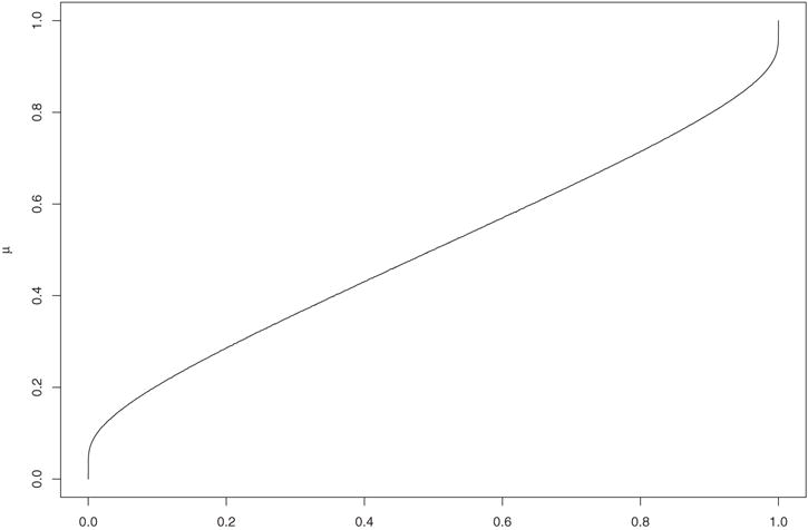
The relationship between the proportion π and the mean μ_Q.

Let X₁ = x₁, X₂ = x₂, …, $X_{n_1}=x_{n_1}$ and Y₁ = y₁, Y₂ = y₂, …, $Y_{n_2}=y_{n_2}$ be two binary samples from Bernoulli distributions, Ber(π₁) and Ber(π₂), respectively. The smooth bootstrap based 100(1 − α)% confidence interval for ralative risk RR = π₁/π₂ may be calculated based on the following algorithm.

1. Calculate the point estimators ${\widehat{\pi }}_1$ and ${\widehat{\pi }}_2$ of π₁ and π₂, respectively. We suggest aforementioned adjusted estimators as an alternative to usual sample proportions.

2. For b = 1, …, B.

   Generate n₁ and n₂ uniformly distributed observations $U_i^{\ast }=u_i^{\ast }$, 1 ≤ i ≤ n₁ and $U_j^{\ast }=u_j^{\ast }$, 1 ≤ j ≤ n₂ from unif(0, 1), respectively.

   Generate the corresponding quantiles $X_i^{\ast }=x_i^{\ast }$, 1 ≤ i ≤ n₁ and $Y_i^{\ast }=y_i^{\ast }$, 1 ≤ j ≤ n₂ by using the estimated quantile function at (2.2) with respect to ${\widehat{\pi }}_1$ and ${\widehat{\pi }}_2$, respectively.

   Calculate the mean $\overline{x}\ast =\frac{1}{n_1}{\displaystyle {\sum }_{i=1}^{n_1}{x}_i^{\ast }}$ and $\overline{y}\ast =\frac{1}{n_2}{\displaystyle {\sum }_{j=1}^{n_2}{y}_i^{\ast }}$

   Calculate $\widehat{R}{R}^{\ast }={\widehat{\pi }}_1^{\ast }/{\widehat{\pi }}_2^{\ast }$, where ${\widehat{\pi }}_1^{\ast }$ and ${\widehat{\pi }}_2^{\ast }$ are obtained by numerically inversing equation (2.4).

3. Calculate the 100×(α/2) percentile ${\widehat{\mathit{RR}}}_{\alpha /2}^{\ast }$ and the 100 × (1−α/2) percentile ${\widehat{\mathit{RR}}}_{1-\alpha /2}^{\ast }$. Then ( ${\widehat{\mathit{RR}}}_{\alpha /2}^{\ast }$, ${\widehat{\mathit{RR}}}_{1-\alpha /2}^{\ast }$) is the 100 × (1 − α)% confidence interval of RR = π₁/π₂.

3. Simulation Study

Simulations studies were conducted in order to compare the performance of our smooth bootstrap method with asymptotic and exact bootstrap methods, in terms of coverage probability and power. Given a specific set of point estimator of two proportions, ${\widehat{\pi }}_1$ and ${\widehat{\pi }}_2$, the sample estimate of the relative risk can be simply expressed as ${\widehat{\pi }}_1/{\widehat{\pi }}_2$. The large sample standard error of $\widehat{\mathit{RR}}$ is estimated by

$$\widehat{\mathit{se}(\widehat{\mathit{RR}})}=\sqrt{\frac{1-{\widehat{\pi }}_1}{n_1{\widehat{\pi }}_1}+\frac{1-{\widehat{\pi }}_2}{n_2{\widehat{\pi }}_2}},$$ (3.1)

and the associated 100(1 − α)% confidence interval is constructed as

$$(\widehat{\mathit{RR}}-z_{1-\alpha /2}\widehat{\mathit{se}(\widehat{\mathit{RR}}))},\widehat{\mathit{RR}}+z_{1-\alpha /2}\widehat{\mathit{se}(\widehat{\mathit{RR}}))},$$ (3.2)

where z_1−α/2 is the 100(1 − α/2)% quantile of standand normal random variable. Carter et al. (2010) compared this large sample method in their simulation studies with their deterministic bootstrap method, where the bootstrap probabilities of (n₁ + 1)(n₂ + 1) elements of the sample space are fully specified. For more details, see Lin et al. (2009) and Carter et al. (2010).

It should be noted that the performance of the various methods for constructing confidence intervals for the relative risk relies on the method for the point estimation of the two respective proportions. Given an observed number x events out of n trials, three common point estimators of the population proportion π are considered in our simulation studies.

1. Jeffreys estimator, defined as $\widehat{\pi }=(x+1)/(n+2)$.

2. The score estimator, defined as $\widehat{\pi }=(x+2)/(n+4)$.

3. The MUE estimator, defined as $\widehat{\pi }=({\widehat{\pi }}^L+{\widehat{\pi }}^U)/2$, where ${\widehat{\pi }}^L$ and ${\widehat{\pi }}^U$ are obtained by solving $\mathrm{Pr}(X\ge x|\pi ={\widehat{\pi }}^L)=0.5$ and $\mathrm{Pr}(X\le x|\pi ={\widehat{\pi }}^U)=0.5$, respectively.

In order to assess the performance of our proposed method under a variety of scenarios, the underlying binomial proportion for the first group was allowed to range from 0.02–0.98 by 0.04 increment and four ratios, π₁/π₂ = 1, 2, and 4, between two groups are considered. Sample sizes of 10, 25, and 50 for each group are included with 1000 replications per simulation scenario. For each generated set of data, the Jeffreys, score, and MUE point estimates of π₁ and π₂ are calculated and the associated confidence intervals are calculated through the asymptotic (LS), exact bootstrap (E-boot), and our smooth bootstrap (S-boot) method. The coverage probabilities of aforementioned methods given different relative risks are displayed in Figs. 2–4. Particularly, Fig. 2 displays the coverage probabilities under the scenario π₁/π₂ = 1. The score estimator has a performance comparable to the Jeffreys estimator. Hence, its results are not shown in order to make the figures more clear. Note that the diagonal subplots in Fig. 2 for the cases of two groups with equal sample sizes have similar shapes as Fig. 2 in Carter et al. (2010). For small (n = 10) to mediate (n = 25) sample sizes, the coverage probabilities of our proposed smooth bootstrap method are quite close to the desired nominal coverage probability of 95% over a large range of π₁. For the large sample size of n = 50, the difference between the exact bootstrap and smooth bootstrap is negligible. Each bootstrap method is better than the asymptotic method in this case. All methods are conservative when binomial proportions are proximate to the boundaries in that their coverage probabilities are greater than the nominal level. The above observations are generally true for cases with either equal or unequal sample sizes. Note that the dotted lines in Figs. 2–6 is used as the reference which represents the confidence intervals derived with the combination of the usual sample proportion $\widehat{\pi }=x/n$ and the asymptotic rule. Figures 3 and 4 share similar pattern. In general, our smooth bootstrap method is closer to the nominal level of 95% than the other two methods. All methods are conservative when π₁ is close to 0. It is worth pointing out that the exact bootstrap method shows surprisingly low coverage probabilities given certain combinations of sample sizes, such as n₁, n₂ = (50, 10) in Fig. 3, and n₁, n₂ = (20, 10) and n₁, n₂ = (50, 10) in Fig. 4. This phenomena have been noted previously, e.g., see Carter et al. (2010).

Figure 2.

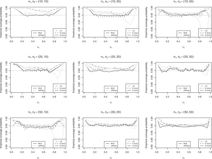
Empirical coverage probability given π₁/π₂ = 1.

Figure 4.

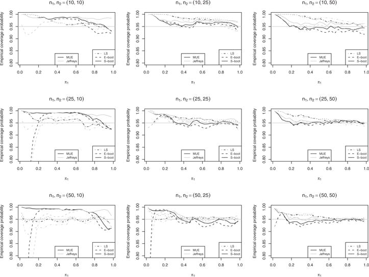
Empirical coverage probability given π₁/π₂ = 4.

Figure 6.

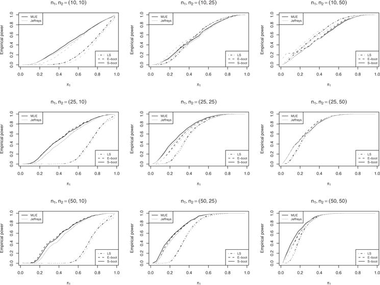
Empirical power given π₁/π₂ = 4.

Figure 3.

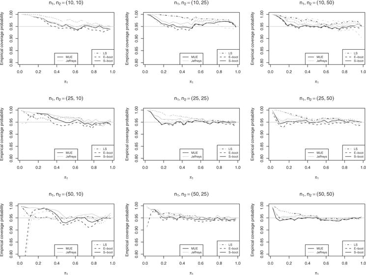
Empirical coverage probability given π₁/π₂ = 2.

The power levels, i.e., the frequency for which the confidence interval contains the alternative value for the relative risk different from π₁/π₂ = 1, is shown in Figs. 5 and 6 for π₁/π₂ = 2 and π₁/π₂ = 4, respectively. Given a specified sample proportion estimator, the power levels of our smooth bootstrap methods are generally higher than or equal to those of the exact bootstrap method, particularly for equal sample size. The large sample method usually has a worse performance than the two bootstrap method, except for the case of n₁, n₂ = (10, 50).

Figure 5.

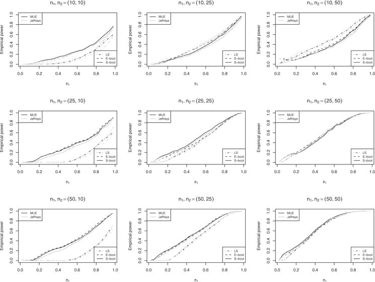
Empirical power given π₁/π₂ = 2.

The overall coverage probabilities for each method are summarized in Tables 1–3 for π₁/π₂ = 1, 2, and 4, respectively. Each cell represents the average coverage probability across all values of π₁. The Wald column represents the coverage probabilities of confidence intervals derived using usual sample proportion estimates $\widehat{\pi }=x/n$ and asymptotic standard error. It is clear that this method usually provides conservative confidence intervals, which is partially due to the decision rule we adopt from Carter et al. (2010); the confidence interval is set to (0, ∞) if 0 event is observed in either group. Given any of the three alternative proportion estimators (MUE, score, and Jeffreys), the large sample method yields more conservative coverage probabilities than the two bootstrap methods under a major portion of scenarios included in our simulation study. Our smooth bootstrap method is slightly conservative and tends to be closer to the nominal level of 95% than the large sample method. The exact bootstrap method seems to be closest to the nominal level, but this is mainly due to the trade-off between relative high coverage at both boundaries and relative low coverage at the middle range. It is worth noting that due to the discrete nature of the exact bootstrap method, it could have a very poor performance given unequal sample sizes, such as n₁, n₂ = (20, 10) and n₁, n₂ = (50, 10) in this article.

Table 1.

π₁/π₂ = 1

n1	n2	Wald LS	MUE			Score			Jeffreys
			LS	E-boot	S-boot	LS	E-boot	S-boot	LS	E-boot	S-boot
10	10	0.987	0.992	0.97	0.965	0.999	0.993	0.987	0.996	0.979	0.97
10	25	0.958	0.976	0.957	0.962	0.989	0.976	0.984	0.979	0.969	0.975
10	50	0.934	0.965	0.954	0.966	0.982	0.925	0.983	0.972	0.962	0.974
25	10	0.963	0.978	0.961	0.964	0.99	0.973	0.983	0.98	0.969	0.975
25	25	0.973	0.977	0.97	0.953	0.983	0.981	0.974	0.98	0.975	0.962
25	50	0.962	0.969	0.955	0.956	0.977	0.967	0.97	0.972	0.96	0.963
50	10	0.927	0.958	0.947	0.959	0.974	0.918	0.981	0.964	0.956	0.969
50	25	0.964	0.97	0.957	0.958	0.978	0.969	0.972	0.973	0.961	0.965
50	50	0.96	0.963	0.962	0.949	0.971	0.971	0.962	0.966	0.966	0.956

Table 3.

π₁/π₂ = 4

n1	n2	Wald LS	MUE			Score			Jeffreys
			LS	E-boot	S-boot	LS	E-boot	S-boot	LS	E-boot	S-boot
10	10	0.969	0.969	0.953	0.977	0.949	0.831	0.985	0.964	0.961	0.986
10	25	0.986	0.981	0.963	0.967	0.976	0.941	0.978	0.976	0.96	0.975
10	50	0.979	0.979	0.942	0.951	0.98	0.946	0.971	0.984	0.953	0.967
25	10	0.959	0.959	0.9	0.981	0.926	0.738	0.987	0.941	0.888	0.988
25	25	0.97	0.967	0.947	0.959	0.95	0.903	0.974	0.96	0.955	0.97
25	50	0.971	0.969	0.952	0.956	0.962	0.943	0.966	0.965	0.958	0.962
50	10	0.952	0.947	0.912	0.98	0.912	0.7	0.986	0.932	0.869	0.988
50	25	0.961	0.955	0.931	0.957	0.926	0.869	0.971	0.948	0.937	0.966
50	50	0.963	0.961	0.939	0.949	0.953	0.927	0.963	0.961	0.949	0.957

4. Example

We illustrate the application of our smooth bootstrap method via utilizing the example presented in Carter et al. (2010), which is derived from three interim reports of a clinical trial in order to compare the likelihood of a severe hypoglycemic event between intensive and standard glycemic control. The data are used by the original authors to illustrate MUE based relative risk estimators and exact bootstrap methods to construct the associated confidence intervals when only a very small number of events are observed in each group. This is traditionally a situation where MLE method for estimation is ill behaved. We re-analyzed the data to compare different methods for constructing confidence intervals given a certain type of proportion estimator. Table 4 shows the 95% confidence intervals for the large sample (LS), exact bootstrap (E-boot) and new smooth bootstrap (S-boot) methods. Compared with the confidence intervals generated from large sample theory, those generated by the exact bootstrap method are much narrower, whereas those generated by the smooth bootstrap are much wider. We argue that confidence intervals generated from our smooth bootstrap are more appropriate for this kind of data given issues relative to the underlying discreteness of the other approaches in the small sample setting. Consider the first set of data with ${\displaystyle {\sum }_{i=1}^{n_1=3}{x}_i=0}$ and ${\displaystyle {\sum }_{i=1}^{n_2=4}{y}_i=0}$ events in each group, the probability of having this observation given π₁ = 0.01 and π = 10⁻⁷ with RR = π₁/π₂ = 10⁵ is as high as 97%. Therefore RR = 10⁵ deserves to be included into the final 95% confidence interval. Furthermore, note that the 95% Wilson score intervals for π₁ and π₂ given 0/3 and 0/4 are ${\mathrm{CI}}_{{\pi }_1}=(0,0.69)$ and ${\mathrm{CI}}_{{\pi }_2}=(0,0.60)$, respectively. A reasonable confidence interval of RR = π₁/π₂ would be approximated to

$$\left(\frac{\text{lower}\text{bound}\text{of}{\text{CI}}_{{\pi }_1}}{\text{upper}\text{bound}\text{of}{\text{CI}}_{{\pi }_2}},\frac{\text{upper}\text{bound}\text{of}{\text{CI}}_{{\pi }_1}}{\text{lower}\text{bound}\text{of}{\text{CI}}_{{\pi }_2}}\right)$$

after certain multiple testing adjustment; see more details about constructing simultaneous confidence intervals for binomial proportions in Agresti et al. (2008). Towards this end, consider the third set of data with ${\displaystyle {\sum }_{i=1}^{n_1=12}{x}_i=1}$ and ${\displaystyle {\sum }_{i=1}^{n_1=15}{y}_i=1}$ events in each group, the 95% Wilson score intervals for π₁ and π₂ are ${\text{CI}}_{{\pi }_1}=(0.0044,0.40)$ and ${\text{CI}}_{{\pi }_2}=(0.0035,0.34)$, respectively. The probability of observing more favorable data, such as ${\displaystyle {\sum }_{i=1}^{n_1=12}{x}_i\ge 1}$ and ${\displaystyle {\sum }_{i=1}^{n_2=15}{y}_i\le 1}$, given π₁ = 0.4 and π₂ = 0.004 with RR = π₁/π₂ = 100 is as high as $\mathrm{Pr}({\displaystyle {\sum }_{i=1}^{n_1=12}{x}_i\ge 1})\mathrm{Pr}({\displaystyle {\sum }_{i=1}^{n_2=15}{y}_i\le 1})=98\%$. We note that our method is consistent with the classic score method developed by Koopman (1984), from which the confidence intervals are derived as (0, ∞), (0, ∞), and (0.14, 11.22) for the three sets of data, respectively. Seemingly, both large sample and exact bootstrap methods give more credit to the data than it deserves.

Table 4.

95% confidence intervals for RR = π₁/π₂

		$\begin{array}{l}{\displaystyle {\sum }_{i=1}^{n_1=3}=0}\\ {\displaystyle {\sum }_{i=1}^{n_2=4}=0}\end{array}$	$\begin{array}{l}{\displaystyle {\sum }_{i=1}^{n_1=9}{x}_u=1}\\ {\displaystyle {\sum }_{i=1}^{n_2=11}{y}_i=0}\end{array}$	$\begin{array}{l}{\displaystyle {\sum }_{i=1}^{n_1=12}{x}_u=1}\\ {\displaystyle {\sum }_{i=1}^{n_2=15}{x}_u=1}\end{array}$
MUE	LS	(0.012, 145)	(0.098, 176)	(0.11, 14.6)
	E-boot	(0.21, 8.06)	(0.35, 13.89)	(0.13, 11.46)
	S-boot	(3.96e-05, 25500)	(0.023, 15800)	(0.019, 82.3)
Score	LS	(0.051, 28)	(0.2, 28)	(0.17, 8.62)
	E-boot	(0.33, 3.05)	(0.38, 5.36)	(0.29, 4.65)
	S-boot	(4.84e-05, 22200)	(0.11, 1410)	(0.066, 22.4)
Jeffreys	LS	(0.019, 83)	(0.14, 91.3)	(0.13, 11.3)
	E-boot	(0.23, 4.05)	(0.4, 8.36)	(0.17, 8.11)
	S-boot	(4.22e-05, 26700)	(0.066, 13200)	(0.033, 34.9)

Even though it is not the focus of this article, it is seen that the width of the confidence interval depends on the method of estimating the two proportions. Score estimators are usually associated with the narrowest intervals while MUE estimators are associated the widest intervals. We also note that for relative frequent event rate, such as 4/12 vs. 5/15, the difference between the three methods are negligible.

5. Summary and Discussion

In this article, we develop a new resampling procedure to construct confidence intervals for the relative risk given pre-specified pairs of sample proportion estimators. The resulting confidence interval is “smooth bootstrap like” in terms of it properties with respect to the generation of pseudo-observations from a smooth quantile function defined in Wang and Hutson (2011). In our simulation studies, the performance of our smooth bootstrap method is usually better than the classic asymptotic theory based method and the commonly used exact bootstrap method, in terms of coverage probability and power. Particularly, when the two groups are seriously unbalanced, the coverage probabilities of confidence intervals from exact bootstrap method could be much lower than the nominal confidence level. As mentioned in Carter et al. (2010), this is possibly because the deterministic bootstrap sample space will be more defined by the larger group’s sample size.

Through a previously published example, we show that given very low event rate and small sample size, confidence intervals generated from smooth bootstrap method are much more wider than those from asymptotic method whereas those from exact bootstrap method are much narrower. We note that the results from our method are consistent with the classic score method proposed in Koopman (1984) and suggest conservative confidence intervals for this type of data. In addition, the smooth bootstrap method can be readily extended towards constructing the confidence intervals for odds ratios.

It should also be mentioned that the interval estimators considered in this note is a limited portion of currently available methods for relative risk, which are chosen towards assessing and evaluating the proposed smooth bootstrap method in comparison with the asymptotic rule and exact bootstrap method. Given a specific set of data, Koopman’s classic score interval and the exact unconditional interval proposed by Agresti and Min (2005) are generally recommended. We also recommend the method proposed by Price and Bonett (2008) with respect to its ease of being implemented and satisfactory performance comparable to the Koopman’s score method; see more comparisons and discussions about inference methodologies for relative risk in Price and Bonett (2008) and Fagerland et al. (2011).

Table 2.

π₁/π₂ = 2

n1	n2	Wald LS	MUE			Score			Jeffreys
			LS	E-boot	S-boot	LS	E-boot	S-boot	LS	E-boot	S-boot
10	10	0.978	0.977	0.955	0.962	0.977	0.97	0.983	0.977	0.962	0.966
10	25	0.982	0.985	0.959	0.963	0.986	0.961	0.98	0.986	0.958	0.972
10	50	0.97	0.974	0.953	0.956	0.987	0.951	0.974	0.98	0.954	0.964
25	10	0.963	0.963	0.95	0.963	0.964	0.913	0.983	0.962	0.96	0.972
25	25	0.969	0.97	0.951	0.954	0.972	0.969	0.971	0.971	0.959	0.963
25	50	0.97	0.969	0.945	0.955	0.972	0.955	0.964	0.97	0.952	0.961
50	10	0.951	0.954	0.913	0.961	0.944	0.872	0.983	0.951	0.918	0.972
50	25	0.96	0.959	0.943	0.953	0.957	0.95	0.969	0.958	0.949	0.96
50	50	0.96	0.959	0.948	0.947	0.96	0.959	0.96	0.959	0.952	0.954

References

- Agresti A, Bini M, Bertaccini B, Ryu E. Simultaneous confidence intervals for comparing binomial parameters. Biometrics. 2008;64:1270–1275. doi: 10.1111/j.1541-0420.2008.00990.x. [DOI] [PubMed] [Google Scholar]
- Agresti A, Coull BA. Approximate is better than exact for interval estimation of binomial proportions. Amer Statistician. 1998;52:119–126. [Google Scholar]
- Agresti A, Min Y. On small-sample confidence intervals for parameters in discrete distributions. Biometrics. 2001;57:963971. doi: 10.1111/j.0006-341x.2001.00963.x. [DOI] [PubMed] [Google Scholar]
- Agresti A, Min Y. Frequentist performance of Bayesian confidence intervals for comparing proportions in 22 contingency tables. Biometrics. 2005;61(2):515–523. doi: 10.1111/j.1541-0420.2005.031228.x. [DOI] [PubMed] [Google Scholar]
- Brown LD, Cai TT, DasGupta A. Interval estimation for a binomial proportion. Statist Sci. 2001;16(2):101–133. [Google Scholar]
- Carter RE, Lin Y, Lipsitz SR, Hermayer KL. Relative risk estimated from the ratio of two median unbiased estimates. J Roy Statist Soc Seri C Appl Statist. 2010;59:657–671. doi: 10.1111/j.1467-9876.2010.00711.x. [DOI] [PMC free article] [PubMed] [Google Scholar]
- Fagerland MW, Lydersen S, Laake P. Recommended confidence intervals for two independent binomial proportions. Statist Meth Med Res. 2011 doi: 10.1177/0962280211415469. [DOI] [PubMed] [Google Scholar]
- Hirji KF, Tsiatis AA, Mehta CR. Median unbiased estimation for binary data. The Amer Statistician. 1989;43:7–11. [Google Scholar]
- Katz D, Baptista J, Azen SP, Pike MC. Obtaining confidence intervals for the risk ratio in cohort studies. Biometrics. 1978;34:469–474. [Google Scholar]
- Koopman PAR. Confidence intervals for the ratio of two binomial proportions. Biometrics. 1984;40:513–517. [PubMed] [Google Scholar]
- Lin Y, Newcombe RG, Lipsitz S, Carter RE. Fully specified bootstrap confidence intervals for the difference of two independent binomial proportions based on the median unbiased estimator. Statist Med. 2009;28:2876–2890. doi: 10.1002/sim.3670. [DOI] [PubMed] [Google Scholar]
- Newcombe RG. Two-sided confidence intervals for the single proportion: comparison of seven methods. Statist Med. 1998;17:857–872. doi: 10.1002/(sici)1097-0258(19980430)17:8<857::aid-sim777>3.0.co;2-e. [DOI] [PubMed] [Google Scholar]
- Parzen M, Lipsitz S, Ibrahim J, Klar N. An estimate of the odds ratio that always exists. J Computat Graph Statist. 2002;11:420–436. [Google Scholar]
- Price RM, Bonett DG. Confidence intervals for a ratio of two independent binomial proportions. Statist Med. 2008;27:5497–5508. doi: 10.1002/sim.3376. [DOI] [PubMed] [Google Scholar]
- Wang D, Hutson AD. A fractional order statistic towards defining a smooth quantile function for discrete data. J Statist Plann Infer. 2011;141:3142–3150. [Google Scholar]
- Wilson EB. Probable inference, the law of succession, and statistical inference. J Amer Statist Assoc. 1927;22:209–212. [Google Scholar]