Co-activation Probability Estimation (CoPE): An approach for modeling functional co-activation architecture based on neuroimaging coordinates

Abstract

Recent progress in functional neuroimaging has prompted studies of brain activation during various cognitive tasks. Coordinate-based meta-analysis has been utilized to discover the brain regions that are consistently activated across experiments. However, within-experiment co-activation relationships, which can reflect the underlying functional relationships between different brain regions, have not been widely studied. In particular, voxel-wise co-activation, which may be able to provide a detailed configuration of the co-activation network, still needs to be modeled. To estimate the voxel-wise co-activation pattern and deduce the co-activation network, a Co-activation Probability Estimation (CoPE) method was proposed to model within-experiment activations for the purpose of defining the co-activations. A permutation test was adopted as a significance test. Moreover, the co-activations were automatically separated into local and long-range ones, based on distance. The two types of co-activations describe distinct features: the first reflects convergent activations; the second represents co-activations between different brain regions. The validation of CoPE was based on five simulation tests and one real dataset derived from studies of working memory. Both the simulated and the real data demonstrated that CoPE was not only able to find local convergence but also significant long-range co-activation. In particular, CoPE was able to identify a ‘core’ co-activation network in the working memory dataset. As a data-driven method, the CoPE method can be used to mine underlying co-activation relationships across experiments in future studies.

Introduction

Over the past two decades, researchers have used neuroimaging to study the functional and structural aspects of the brain, leading to the generation, analysis, and publication of large amounts of data. Consequently, large scale accessible databases, such as BrainMap (Fox & Lancaster, 2002; Laird et al., 2005) and NeuroSynth (Yarkoni et al., 2011), which compile published neuroimaging results, have arisen as repositories for the various types of information including peak coordinates obtained from neuroimaging studies. The use of functional magnetic resonance imaging (fMRI) and diffusion tensor imaging (DTI) has helped to generate great interest in investigating the functional and structural connectivity of the human brain. Although the number of connectivity-based neuroimaging studies that employed tasks is fewer than the ones that studied the resting state, the growing number of these task-based studies provides a significant opportunity to expand our knowledge of task-dependent functional connectivity in order to identify “emergent properties”, i.e., to discover classes of observations not reported in the source publications (Fox & Friston, 2012; Laird et al., 2013).

In the first such study, Toro et al. (2008) used chi-square calculations to investigate the relationship between the task-dependent co-activation pattern and canonical functional brain networks, such as the default mode network. As meta-analytic techniques have improved, the evolving family of coordinate-based meta-analysis (CBMA) methods has offered data-driven techniques to quantitatively synthesize the consistent functional activation. In general, CBMA is based on three-dimensional coordinates in MNI (Evans et al., 1992) or Talairach (Talairach & Tournoux, 1988) standard reference space. Common CBMA methods are activation likelihood estimation (ALE; (Eickhoff et al., 2012; Eickhoff et al., 2009; Turkeltaub et al., 2002)) and related techniques, such as (multilevel) kernel density analysis (KDA and MKDA; (Wager et al., 2004; Wager et al., 2007)). A new meta-analytic technique based on ALE, meta-analytic connectivity modeling (MACM), is able to investigate task-dependent connectivity (Eickhoff et al., 2010; Laird et al., 2009; Robinson et al., 2010). In principle, MACM is a seed-based method which estimates the activation-dependent connectivity for a user-defined region of interest. Another method, independent component analysis (ICA), can be used to mine the architecture of task-dependent networks in the BrainMap database. The task-dependent networks also match the pattern from resting state fMRI data from healthy subjects (Ray et al., 2013; Smith et al., 2009). Other researchers (Poldrack et al., 2012) used a topical mapping method to extract the task-dependent networks from the NeuroSynth database. The networks they obtained were also similar to the networks obtained using resting state data (Poldrack et al., 2012).

These previously-mentioned methods could deduce significantly convergent activated regions and interpret them as network distributions. However, these methods may have disadvantages when configuring a detailed connectivity pattern between any two activated brain regions or voxels. Specifically, the MACM method, which is based on defining a region of interest, i.e., a seed-based method, may not be feasible if the integration or co-activation between any two seeds is taken into account because the co-activations will need to be calculated one by one. The other method, i.e., the ICA-based method, can identify the architecture of a task-dependent co-activation network, but the configuration of the network may not be detected, i.e., all of the above-threshold brain regions identified using the ICA-based method may be considered as consistently co-active. For example, if the ICA-based method found that brain regions A, B, and C were above the threshold, a situation could quite possibly exist in which A and B are co-activated, and B and C are also co-activated, but A and C are not co-activated. In this situation, the two activated brain regions did not have the same connectivity or functional co-activation relationships. On the other hand, the ICA-based method necessitates using a large number of experiments to satisfy the sample size demanded by the ICA method. For example, a specific cognitive dataset, such as one using experiments about working memory, might not have a sufficient number of experiments, causing sample size to be a problem.

In order to determine the voxel-wise configuration of co-activation networks, we proposed a method we called CoPE, which modeled the activation around peak foci by making a map of the Gaussian distribution around each focus within each experiment. Using co-occurrence within the same experiment as the criterion, CoPE defined the voxel-wise co-activations across the experiments. Then, a permutation test was introduced into CoPE as a significance test. Further, CoPE could separate the co-activation patterns into either local or long-range, based on a well-defined distance. On one hand, local co-activation reflects local convergence in a manner similar to that of the ALE method. Local co-activation is mainly generated from the model. On the other hand, long-range co-activation reflects consistent within-experiment co-activation between distant regions. Mining the interaction effects of the underlying task-dependent network is of particular interest. To evaluate the CoPE method, we employed five simulation datasets and a real working memory dataset to test whether the method could mine the architecture and the configuration, i.e., the co-activation relationship, of the co-activation network, especially long-range patterns from large datasets.

Materials and methods

In practice, few neuroimaging experiments can report more than a dozen foci for a given contrast, i.e., the activation foci are sparsely distributed around the brain. So, CoPE only takes co-activations into account, i.e., non-occurrences between two foci are not modeled. There are three steps in the CoPE method: The first is to map the peak foci onto activation maps after calculating the Gaussian distribution around each focus within each experiment. The second step is to obtain the weight of the co-activation between any two voxels using the individual activation map from step 1. The third step is to perform a permutation test to determine the significance of the co-activation. Fig. 1 gives an overview of the CoPE method.

Fig. 1.

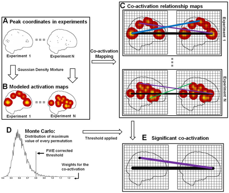
Schematic representation of the procedures for CoPE. (A) Identifying the peak coordinates from N experiments. (B) Treating each peak coordinate in each experiment separately as the center of a 3D Gaussian probability distribution and combining the distribution functions to provide a specific density function for each experiment. The density in each voxel was used to model the activation in each experiment. (C) Defining the voxel-wise co-activation relationships. In each experiment, the lines (for example, the black line) represent co-activation between the voxels at each end. (D) Deriving the null-distribution which can reflect the random spatial co-activation across experiments. The peak coordinates in each experiment were randomly permutated, and the maximum value of the co-activation from each permutation was used to create a random co-activation map with which to compare the actual co-activation map. (E) Deriving the voxel-based significant co-activation relationships. All the co-activation relationship maps were pooled, and the threshold for the pooled weight of each line was used to identify the lines that represented significant co-activation (for example, the black and the purple ones).

Mapping the peak foci

Like the ALE method, CoPE uses a three-dimensional Gaussian distribution to model activation around individual coordinates. So, let $C_i=\{C_1^i\dots C_{n_i}^i\}$ be the reported foci in the ith experiment, where n_i is the number of foci in the ith experiment. Let $\mathrm{G}(C_j^i,{\sum }_i)$ represent a three-dimensional Gaussian distribution centered at coordinate $C_j^i$, where Σ_i is the three-dimensional diagonal covariance matrix. The elements on the diagonal are the same and can be defined according to the empirical estimates provided by Eickhoff et al. (2009). The empirical estimate is based on the inter-subject and inter-template variability. In order to assess the modeled activation distribution in one experiment, the Parzen-window density estimation method (Parzen, 1962; Rosenblatt, 1956) was adopted to model the activation map. In this way, let AM_i be the activation map for the ith experiment, where AM_i can be formalized as

$${\mathit{\text{AM}}}_i(\mathrm{v})=\frac{1}{n_i}\sum _{j=1}^{n_i}\mathrm{G}(\mathrm{v};C_j^i,{\sum }_i)$$

with v denoting a voxel. This process was repeated to form an activation map for each experiment.

Modeling the voxel-wise co-activations

The co-activation relationship, i.e., the activated coordinates reported in a single experiment, is the key idea behind CoPE. In theory, the definition of co-activation between two voxels could be the product of the individual probabilities of the activations from the activation map, i.e., the estimated probability density function (pdf), for the experiment. However, accuracy will be an issue if the probability is directly generated from the estimated pdf. Because the voxel resolution used in CoPE is 2 × 2 × 2 mm, the estimated pdf will contain a lot of small values for a large number of voxels, causing problems with accuracy if these are multiplied by each other. More importantly, the significance test in next step will need a much higher accuracy to distinguish the difference between co-activation weights, if we define the co-activation as the direct product of probabilities from the estimated pdf. In addition, each experiment was considered as independent, and, the experiments need to be comparable. So, a normalization procedure was adopted to increase the comparability between experiments. In detail, let V = {v₁, …, v_nv} be the voxel set, where n_v is the number of voxels. So, the normalized activation weight for the voxel x in the ith experiments can be defined as

$$P_i(v_x)=\frac{{\mathit{\text{AM}}}_i(v_x)}{{\mathit{\text{AM}}}_i(v_x)+max({\mathit{\text{AM}}}_i(v_x))}$$

where P_i(v_x) is the normalized weight for the activation at voxel x in the ith experiment. The max (AM_i(v_x)) is the maximum weight for the activation in the ith experiment. The nonlinear form of normalization is based on the consideration which is to emphasize the activation weight close to the informative part (the part of high activation weight) in a given experiment. After converting the probability density into the normalized activation weight, the weight of the co-activation between any two voxels across experiments can be defined as

$${\text{CoW}}_{x\_y}=\sum _{i=1}^{n_{\mathit{exp}}}{P}_i(v_x)\ast P_i(v_y)$$

where CoW_{x_y} represents the co-activation weight between voxels x and y across experiments. n_exp is the number of the experiments. The necessity of the normalization is illustrated by the calculation of CoW_{x_y}, which guarantees the accuracy of the calculation. Obviously, co-activations with high weights correspond to a high probability of consistency among the experiments.

Inference based on the permutation test

Due to the nonlinear calculation of CoW_{x_y}, a parametric inference based on the Gaussian random field was not feasible (Eickhoff et al., 2012). In addition, the false discovery rate (FDR) is not the optimal approach for making inferences about the topological features derived from ALE-like meta-analysis methods (Eickhoff et al., 2012). So, the nonparametric family-wise error rate (FWE) correction for multiple comparisons was used. More specifically, the nonparametric FWE correction was based on a Monte-Carlo analysis, i.e., the reported coordinates in each experiment are randomly redistributed throughout the gray matter of the brain in each permutation. The gray matter mask was based on ICBM (The International Consortium for Brain Mapping) gray matter maps with a probability above 10% (Evans et al., 1994). In each permutation, the number of coordinates and the number of subjects in each experiment were kept unchanged. The co-activation weight between voxels, i.e., CoW_{x_y}, was calculated in each permutation. The maximum value of CoW_{x_y} was preserved for subsequent inference. To this end, the distribution of the maximum co-activation weight was used for the FWE correction (Nichols & Hayasaka, 2003). In fact, if the distribution of the maximum redistributed co-activation weight is calculated strictly as mentioned earlier, the time cost will be too high. For example, performing 5000 permutations on a dataset of about 180 experiments and about 3000 coordinates would take one to two days to calculate using a computer running at 2.4 GHz with 16 GB of memory. Here, we provided an alternative approach for estimating the compact upper bound of the maximum co-activation weight in each permutation. Replacing the maximum co-activation weight with the upper bound allowed us to save a great deal of calculation cost while providing a conservative estimate of the FWE correction. More precisely, the key idea behind the approach is based on the Cauchy–Schwarz inequality (Kadison, 1952; Steele, 2004), in which the calculation of the co-activation weight satisfies

$${\mathit{\text{CoW}}}_{x\_y}^k=\sum _{i=1}^{n_{\mathit{exp}}}{P}_i(v_x,k)\ast P_i(v_y,k)\le \sqrt{\sum _{i=1}^{n_{\mathit{exp}}}{P}_i{(v_x,k)}^2\sum _{i=1}^{n_{\mathit{exp}}}{P}_i{(v_y,k)}^2}=\mathit{\text{up}}\_{\mathit{\text{CoW}}}_{x\_y}^k$$

where ${\mathit{\text{CoW}}}_{x\_y}^k$ is the co-activation weight between any two voxels in the kth permutation. P_i(v_x, k) > 0 and P_i(v_y, k) > 0 are the normalized weights of the activations within the ith experiment at any voxel in the kth permutation. $\mathit{\text{up}}\_{\mathit{\text{CoW}}}_{x\_y}^k$ is the upper bound of ${\mathit{\text{CoW}}}_{x\_y}^k$. After the conversion, the maximum value of the co-activation weight in each permutation is calculated by the simplified formula

$${\mathit{\text{CoW}}}_{\mathit{max}}^k\le max(\mathit{\text{up}}\_{\mathit{\text{CoW}}}_{x\_y}^k)$$

where ${\text{CoW}}_{\mathit{max}}^k$ represents the maximum co-activation weight in the kth permutation. The calculation of the maximum of $\mathit{\text{up}}\_{\mathit{\text{CoW}}}_{x\_y}^k$ is based on the descending sort of $\sum _{i=1}^{n_{\mathit{exp}}}{P}_i{(v_x,k)}^2$ across all voxels. After sorting, the product of the first two values in the descending order corresponds to the maximum of $\mathit{\text{up}}\_{\mathit{\text{CoW}}}_{x\_y}^k$.

Local convergence and long-range co-activation

In fact, the co-activations for each voxel fall into two types defined by distance: local convergence and long-range co-activation. In the case of local convergence, the co-activation weight between the peak coordinate and the local neighborhood directly around it should be high, because the coordinate is modeled by the activations that fit a Gaussian distribution. However, our particular interest was to mine the interaction effect of the underlying task-dependent network, which is represented by long-range co-activations. The distance used to distinguish the local and the long-range co-activation was defined as

$$\mathrm{D}=3\delta$$

where D is the distance (in mm) for distinguishing between local convergence and long-range co-activation, and, $\delta =\sqrt{\frac{{7.3}^2}{\sqrt{\overline{N_{\mathit{\text{subj}}}}}}+{3.6}^2}\cdot \overline{N_{\mathit{\text{subj}}}}$ is the mean number of subjects across the experiments. δ is the empirical estimate of the standard deviation for the modeled Gaussian distribution (Eickhoff et al., 2009). Voxels that were 3δ away from the reported focus were considered to be distant, because the probability of their being physically near the focus was negligible. Consequently, co-occurrences beyond this range would not be likely to be driven by a local convergence of the foci but rather represent true co-activation. In order to measure the level of significant co-activation amount at each voxel, the weights of all the significant co-activations with that voxel were added together. The degree density map (DDM) was defined as a map of the summed weights for each voxel. An example of the calculation of a DDM is provided in Supplemental Fig. 1. Further, each DDM was separated into two parts: local and long-range. Specifically, the local DDM was defined as the whole brain degree distribution restricted by distance D, i.e., only local convergence was considered. The long-range DDM referred to the whole brain co-activation distribution beyond distance D, i.e., only long-range co-activations were considered.

Evaluation of the CoPE method

To evaluate the CoPE method, we analyzed several simulated datasets. In addition, we analyzed a real dataset about working memory to see if we could use the reported coordinates to determine the configuration of the task-dependent co-activation network. The ability of CoPE to find the convergent activation regions was validated by comparing the CoPE results with those found using ALE. The simulated datasets had two basic properties in common. First, the simulated peak foci in each experiment were randomly derived from a special Gaussian distribution centered at a designated center. In each experiment, the standard deviation for the Gaussian distribution was calculated using the method in Eickhoff et al. (2009). Second, the number of subjects in each experiment was randomly generated, with a range of 14 to 30 participants.

Each of the five simulations for the CoPE method had some type of special property. Simulation 1 was designed to test whether CoPE could find the convergent activation region across a set of experiments. Convergent activation was a necessary condition for the co-activation analysis in the next step. In this case, an extreme situation in which only one peak focus was found in each experiment was considered. By using only one focus, we could ensure that there was no co-activation between reported foci. Any voxel-wise ‘co-activation’ came completely from the model. Although it only used the modeled co-activation, Simulation 1 was expected to show whether the convergent region was similar to the activation results obtained using ALE. More specifically, the dataset consisted of 50 experiments, each of which included 1 reported coordinate that was randomly derived from the Gaussian distribution centered at this location: MNI: 0 8 64.

Simulation 2 was an expansion of Simulation 1 to test whether CoPE could detect not only multiple convergent activation regions but also the co-activation relationship across different regions. Specifically, we designed 50 experiments in each of which were two reported coordinates randomly derived from two individual Gaussian distributions centered at two centers: Simulated point 1 (SP1, MNI: 0 8 64) and Simulated point 2 (SP2, MNI: 0 -76 6).

Simulation 3 was a supplement to Simulation 2 to determine whether CoPE could distinguish an absence of co-activation between two activated regions. Specifically, we designed 100 experiments, 50 of which had one peak coordinate in each experiment randomly derived from the Gaussian distribution centered at Simulated point 1 (SP1, MNI: 0 8 64) and the other 50 of which had one peak coordinate in each experiment with the Gaussian distribution centered at Simulated point 2 (SP2, MNI: 0 -76 6).

The goal of Simulation 4 was to test whether CoPE would be able to detect both local convergence and long-range co-activation. Specifically, we designed three centers: Simulated point 1 (SP1, MNI: 0 -74 8), Simulated point 2 (SP2, MNI: 0 48 12) and Simulated point3 (SP3, MNI: 0 0 54). Once again, we designed 100 simulated experiments, 50 of which had one peak focus from the Gaussian distribution centered at SP3 and the other 50 had two peak foci individually derived from the two Gaussian distribution centered at SP1 and SP2. Thus, in this simulation SP1 and SP2 were co-activated, but SP3 was only activated.

Simulation 5 investigated the effect of noise on CoPE. Specifically, we designed five centers: Simulated point 1 (SP1, MNI: -12 -16 8), Simulated point 2 (SP2, MNI: 12 -18 6), Simulated point 3 (SP3, MNI: -56 -16 36), Simulated point 4 (SP4, MNI: 56 -16 36) and Simulated point 5 (SP5, MNI: 0 6 60) with five random noise levels: Level 1 (noise coordinates to information coordinates: 10:1), Level 2 (noise coordinates to information coordinates: 3:1) and Level 3 (noise coordinates to information coordinates: 1:1). Two additional levels were also tested to test the extremes. One of these had no random noise and the other had an extreme noise level, in which the ratio of noise coordinates to informative coordinates was 100:1. In all, each simulation utilized 100 experiments, 50 of which had two peak foci individually derived from the two Gaussian distributions centered at SP3 and SP4. The other 50 experiments utilized three peak foci derived separately from SP1, SP2 and SP5. The random noise called for by each noise level was added to each experiment so that it was uniformly distributed across the brain mask.

The real dataset was obtained from a recent coordinate-based meta-analysis on working memory (Rottschy et al., 2012). This dataset consisted of 189 experiments with 2662 activation foci. Differences in the reported coordinates were transformed from Talairach space to MNI space using the Lancaster transform (Lancaster et al., 2007). The dataset had been collected by hand from the BrainMap dataset and the PubMed literature (see more detail in Rottschy et al., 2012).

ALE and CoPE were applied to the simulation datasets and the working memory dataset. ALE was performed by the GingerALE desktop application (http://www.brainmap.org/ale) using the approach provided in Eickhoff et al. (2012) and Eickhoff et al. (2009). The correction method used in ALE was a cluster-level FWE correction. The cluster was formed using a voxel-level threshold of p < 0.001. In the CoPE method, a permutation test with 5000 permutations was used to control the FWE rate.

Results

Simulation datasets

Simulation 1 was used to discover whether CoPE could find the convergent activation region across the experiments. The DDM that revealed the modeled co-activation found by using CoPE was very similar to the activation map from ALE. The pattern of the convergent region obtained using CoPE corresponded to the pattern of the consistently activated region obtained using ALE (Fig. 2A). In addition, the modeled co-activation relationship that passed the FWE correction is shown in Fig. 2B. The modeled co-activation was dense around the simulation point (MNI: 0 8 64).

Fig. 2.

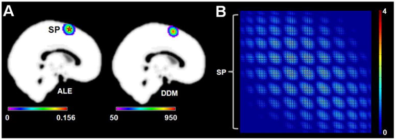
Results of Simulation 1. (A) Left: the ALE results based on the simulation data. The pentagram represents the center (MNI: 0 8 64) of the simulation data. The result was corrected at p < 0.01 using a cluster-level FWE correction. Right: the degree density map (DDM) derived from the FWE-corrected voxel-wise co-activation matrix. (B) The significant voxel-wise co-activation matrix from CoPE. The threshold was p < 0.01 using an FWE correction. Each node of the matrix corresponds to a voxel which had a significant co-activation with other voxels. Each column lists all the significant co-activation relationships that a voxel had with other voxels.

Simulation 2 indicated that CoPE could find the co-activations between different activation regions. Similar regions were detected by both ALE and CoPE (Fig. 3A). Fig. 3B presents the voxel-wise significant co-activation relationships. Consistent with the test design for Simulation 2, co-activation was found between the regions around SP1 and SP2.

Fig. 3.

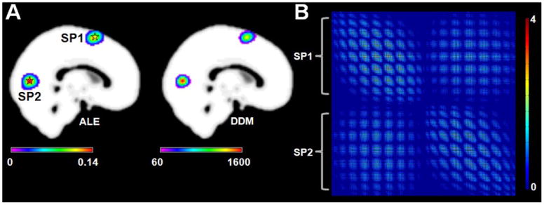
Results of Simulation 2. (A) Left: the ALE results based on the simulation data (p < 0.01, corrected by a cluster-level FWE). The pentagrams represent the centers (MNI: 0 8 64; 0 -76 6) of the simulation data. Right: the degree density map (DDM) derived from the FWE-corrected voxel-wise co-activation matrix. (B) The significant voxel-wise co-activation matrix from CoPE. The threshold was p < 0.01 using an FWE correction. Each nodeofthe matrix correspondedtoa voxel which had a significant co-activation with other voxels. Each column lists all the significant co-activation relationships that a voxel had with other voxels.

As a supplement to Simulation 2, Simulation 3 presented a situation in which the two regions had no co-activations. The activation map from ALE was similar to the DDM from CoPE in Simulation 3 (Fig. 4A). Moreover, the absence of co-activation between the two regions was found by CoPE (Fig. 4B), i.e., there was no co-activation relationship between the regions around SP1 or SP2.

Fig. 4.

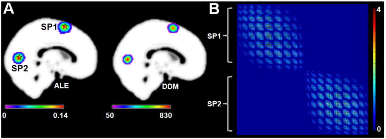
Results of Simulation 3. (A) Left: the ALE results based on the simulation data. The pentagrams represent the centers (MNI: 0 8 64; 0 -76 6) of the simulation data. The result was corrected at p < 0.01 using a cluster-level FWE correction. Right: the degree density map (DDM) derived from the FWE-corrected voxel-wise co-activation matrix. (B) The significant voxel-wise co-activation matrix from CoPE. The threshold was p < 0.01 using an FWE correction. Each node of the matrix corresponded toa voxel which had a significant co-activation with other voxels. Each column lists all the significant co-activation relationships that a voxel had with other voxels.

Simulation 4 was designed to determine whether CoPE could distinguish local convergence from long-range co-activation in the same dataset. Fig. 5A presents the distribution of the dense co-activation regions around the simulated points (SP1, SP2 and SP3). In the simulation, 3δ was used to distinguish between local convergence and long-range co-activation. δ was calculated as described in the Materials and methods section. In the simulation dataset, $\overline{N_{\mathit{\text{subj}}}}$ was 21.3, yielding a 3δ of 11.7 mm. Using this criterion, the local DDM is presented in Fig. 5B, which shows similar distributions around the simulated points. In Fig. 5C, the long-range DDM showed that only the regions around SP1 and SP2 possessed long-range co-activations, a finding which was consistent with the simulation design. The detailed voxel-wise co-activation relationship is presented in Fig. 5D. Meanwhile, this simulation showed no long-range co-activation between SP3 and the others (SP1 and SP2).

Fig. 5.

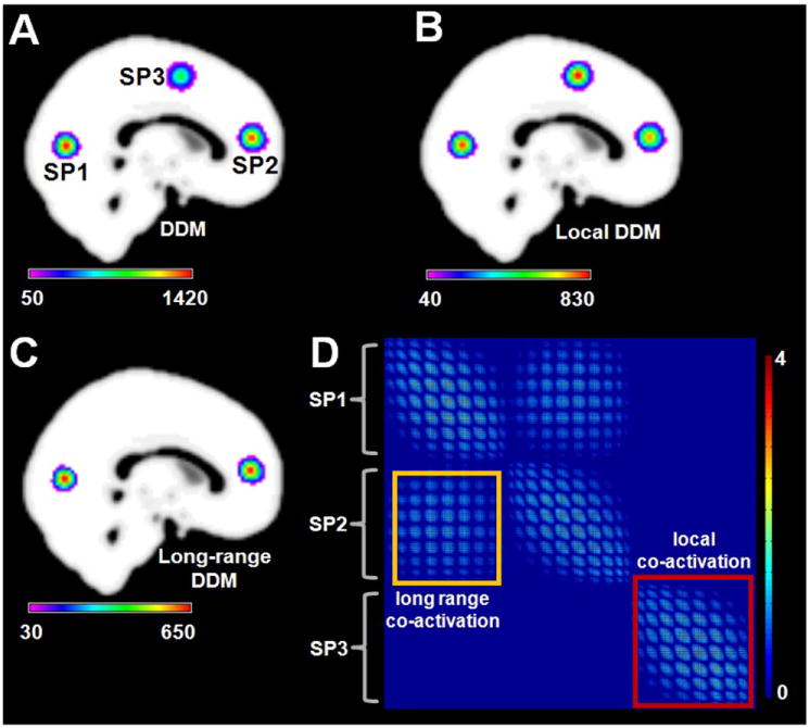
Results of Simulation 4. The co-activation relationship was designed so that the only co-activation relationship was between SP1 and SP2. (A) The degree density map (DDM) derived from the FWE-corrected voxel-wise co-activation matrix. The statistical significance of the co-activation was derived based on an FWE at p < 0.01. The centers of this simulation were at (MNI:0 – 74 8;0 48 12;0 0 54). (B) The local DDM obtained usingthe CoPE method. The co-activations were separated into local and long-range based on a distance of 11.7 mm. (C) The long-range DDM (long DDM) obtained using the CoPE method. (D) The significant voxel-wise co-activation matrix from CoPE. The threshold was p < 0.01 using an FWE correction. Each node of the matrix corresponds to avoxel which had a significant co-activation with other voxels. Each column lists all the significant co-activation relationships that a voxel had with other voxels.

In Simulation 5, simulation datasets with different levels of random noise were used to evaluate the CoPE method. As expected, given the design of the simulation, co-activation occurred between the regions around SP3 and SP4. In addition, the regions around SP1, SP2 and SP5 possessed co-activation relationships between any pair of the regions. CoPE was able to identify co-activation relationships consistent with the design at the different noise levels, although the extent of the co-activations was not precisely the same across the various noise levels. The DDM and the voxel-wise co-activation matrix for the noise-free dataset are presented in Fig. 6A. The co-activation relationship was consistent with the designed one (co-activations between SP1, SP2, and SP5; co-activation between SP3 and SP4). The co-activation relationship was preserved even with an increase in noise level (Fig. 6B–D). Moreover, similarity in the distribution of the regions with dense co-activations was also preserved, although the extent of these regions was a little different from the result from the noise free dataset (DDM in Fig. 6A–D). In the extreme situation (noise: informative foci 100:1), although the co-activation was weaker, the regions corresponding to the design in Simulation 5 could still be found (Supplemental Fig. 2). In detail, little co-activation was found between the region around SP3 and the region around SP4. Co-activation was found between the regions around SP1, SP2, and SP5. Only individual local convergence was found around SP1, SP2, and SP5 (Supplemental Fig. 2).

Fig. 6.

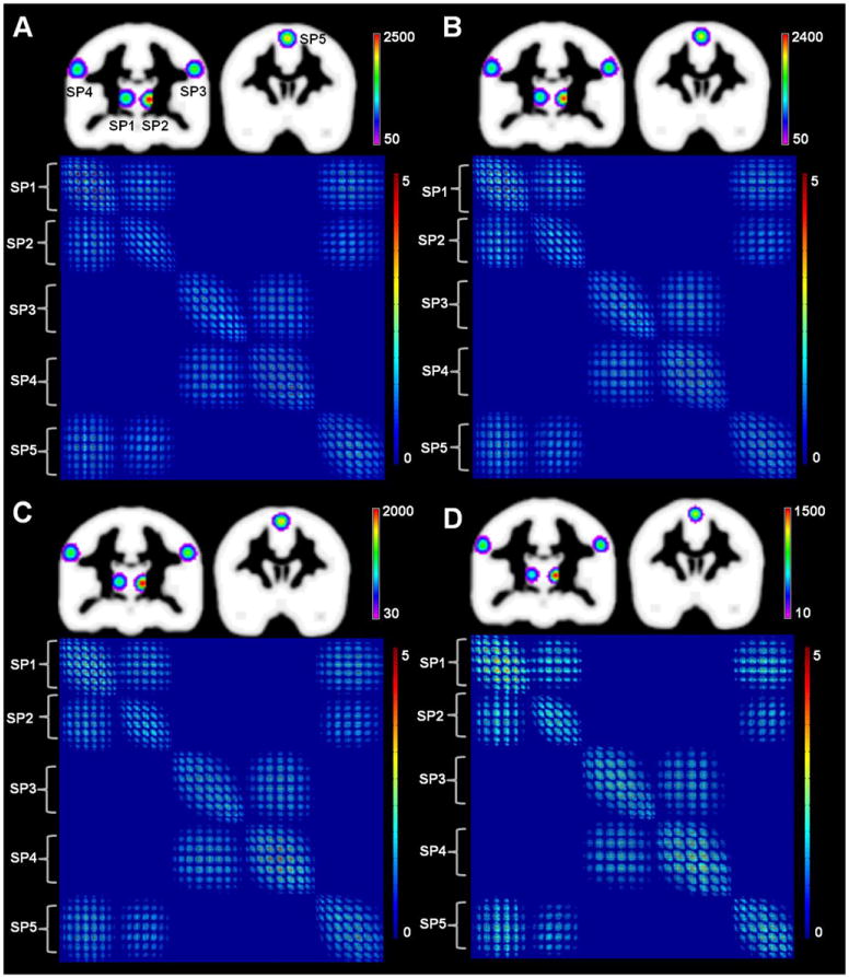
Results of Simulation 5. The data was a simulation around five simulated points, i.e., from SP1 to SP5 (MNI: -12 16 8; 12 -18 6; -56 -16 36; 56 -16 36; 0 6 60). The noise increased from A to D. All of the results are the DDM derived using the CoPE method and the voxel-wise co-activation relationship corrected using an FWE at p < 0.01. (A) Without random noise. (B) The ratio of noise coordinates to information coordinates was 1:1. (C) The ratio of noise coordinates to information coordinates was 3:1. (D) The ratio of noise coordinates to information coordinates was 10:1.

Working memory dataset

The working memory dataset was used to evaluate CoPE in a real application. The long-range co-activations mined from the dataset were particularly interesting in that they showed co-activation relationships between several core brain regions. In detail, the DDM and the local DDM were both similar in the distributions of the significant regions to those obtained using ALE (see Fig. 7A, B, and C). However, the long-range DDM differed from the ALE result when the co-activation was restricted by distance (>12.12 mm; calculated as 3δ based on a $\overline{N_{\mathit{\text{subj}}}}$ of 14.6). Although the ALE and the DDM (Fig. 7A & B, respectively) reflected different aspects of the dataset, they showed similar results. In the ALE result, the significant regions (Fig. 7A) included the bilateral inferior frontal gyrus (IFG; extending to the Broadmann area 44 (BA 44)), the bilateral middle frontal gyrus (MFG), the supplementary motor area (SMA), the bilateral insula (Ins), the bilateral inferior parietal lobule (IPL), the bilateral superior parietal lobule (SPL), the left basal ganglia (BG), the bilateral ventral visual cortex, and lobule VI of the cerebellum. Accordingto the DDM, the regions with a high density (Fig. 7B) were the bilateral IFG (extending to BA44), the bilateral MFG, the SMA, the bilateral Ins, the bilateral IPL, and the bilateral SPL. For the local DDM, the regions with dense local convergence (Fig. 7C) were distributed in the bilateral IFG (extending to BA 44), the bilateral MFG, the SMA, the bilateral Ins, the bilateral IPL, and the bilateral SPL. For the long-range DDM, the main co-activated regions (Fig. 7D) were located in the left IFG (extending to BA44), the SMA, the bilateral Ins, and the left inferior parietal lobule (IPL). Moreover, no significant long range co-activation was found around the right IPG although this had showed up in the results from the ALE and the local DDM (see Fig. 7A, C, and D). The activation extent was smaller in the long-range DDM compared with the local DDM (see Fig. 7C and D). Because long-range co-activation was the main focus of this study, the long-range co-activation was analyzed. In detail, five spatially contiguous clusters were derived from the long-range DDM to define the regions of interest (ROI). We used the criterion of whether a voxel was one of the 26 nearest neighbors to another voxel to determine whether they were in the same ROI or a separate one. The five clusters corresponded to the regions in Fig. 7D and are shown in 3D in Fig. 8B. The voxel-wise long-range co-activation between the clusters is presented in Fig. 8A, which shows the detailed configuration of the co-activation relationship based on the working-memory dataset. In Fig. 8B, the co-activation relationship between any two clusters is shown in 3D. Long-range co-activations were detected between the bilateral Ins, SMA, and left IPL. Between the left BA 44 and the SMA, there was significant co-activation. The long-range core co-activations for the working-memory dataset appeared to form a left-lateralized network, with the exception of the inclusion of the right Ins.

Fig. 7.

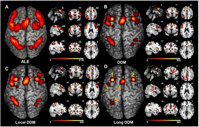
The ALE and CoPE results from the working memory dataset. (A) The ALE results based on the working memory dataset. The threshold was p < 0.05 using a cluster-level FWE correction. (B) The degree density map (DDM) derived from the FWE-corrected voxel-wise co-activation matrix. The statistical significance of the co-activation was derived based on an FWE correction at p < 0.05. (C) The local DDM obtained using the CoPE method. The co-activations were separated into local and long-range based on adistance of 12.12 mm. (D) The long-range DDM (long DDM) obtained using the CoPE method. The numbers represent five clusters based on the criterion of whether a voxel was one of the 26 nearest neighbor voxels.

Fig. 8.

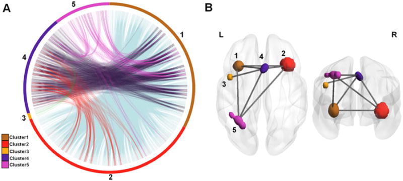
The long-range co-activation relationships derived from the working memory dataset. (A) We identified5 clusters derived from the long-range DDM using the criteria of whether a voxel was one ofthe 26 nearest neighbor voxels. The voxel-wise long-range co-activations were mapped between the clusters. (B) The clusters and the co-activation relationship projected in 3D space.

Discussion

In this current study, we proposed a new approach, which we named CoPE, to infer voxel-wise task-dependent co-activation networks based on coordinates reported in neuroimaging experiments. The significance of the co-activations was identified using a permutation test. The CoPE method was able to distinguish between different types of co-activations, especially between long-range ones and local convergence.

The sparseness of peak foci

CoPE is restricted in modeling the co-activation across experiments. Theoretically, the co-activation and non-co-activation should be equally considered. However, the current experiments usually report only a few foci. It is difficult to distinguish whether the non-reported foci are informative or not. For example, there were 2662 peak foci in the current working memory dataset, but most of these foci (2559) were only reported once. So, we only took the reported foci into consideration. After using the Parzen window density estimation method, we modeled the activation in each experiment. In theory, there was no absolute zero at any voxel no matter how small the activation weight was. Although the approach restricted in activation foci was suboptimal, it obtained more confidence given the special property of the peak foci.

Within-experiments effect

The within-experiments effect refers to the effect of finding multiple foci that are close together and/or of finding many foci in a single experiment. If a study focused on each individual coordinate, i.e., treated each coordinate as independent (a fixed effect), the study could easily be biased by experiments with a greater number of activation coordinates. So, treating individual experiments as independent (a random effect) would help to avoid the within-experiments effect. For the ALE method, Turkeltaub et al. (2012) proposed to set the weight of a voxel according to the nearest reported coordinate in an individual experiment in order to weaken the within-experiments effect. For CoPE, we considered the within-experiments effect differently. Specifically, CoPE used the Parzen window method to estimate the probability density function for each experiment. A normalization procedure was then adopted to increase the comparability between experiments. After normalization, the maximum normalized activation weight was the same in each experiment. In this way, each experiment corresponding to a unique probability distribution function was treated as independent. Even if many foci were reported in one experiment, it was also represented by a probability distribution function, rather than treating the foci as independent.

Multiple comparison correction

As demonstrated in Eickhoff et al. (2012), an FDR correction was not appropriate for inferring the topological features (region of activations) from the statistical map derived from the ALE meta-analysis. So, an FWE correction was adopted in CoPE. By randomly redistributing the coordinates in the experiments and performing the same analysis, the maximum value of each permutation was preserved as an estimate of the distribution of the voxel-level peak values. The estimated distribution could then be used to define the FEW-corrected threshold. This estimation process had the advantage of not needingapre-defined parameterization of the distribution, i.e., it was a non-parameter estimation. FWE correction has been exploited to provide a good estimate of the distribution of the maximum cluster size in the MKDA method (Wager et al., 2007). In the CoPE method, FWE correction was used to provide a voxel-level correction based on the distribution of the maximum co-activation weights from each permutation. However, if the maximum from each permutation was calculated precisely, the computational time would be rather great. Therefore, the Cauchy–Schwarz inequality was used to estimate a conservative upper bound for the maximum for each permutation to reduce the computing cost. In addition, the conservative upper bound provided a more strict correction for the co-activation weight, which was beneficial for the power of the test.

Identification of the local convergence and long-range co-activation

In the CoPE method, the reported coordinates were used as the centers of Gaussian distributions to model activation in the gray matter. Local convergence was reflected by the overlap between the estimated probability density functions. If the local convergence was high around a voxel, CoPE showed that the estimated probability density functions densely overlapped with each other across the experiments. Thus, although local convergence was primarily generated using the model, local convergence could be considered as another way to represent consistent activation across a set of experiments. Long-range co-activations were particularly interesting, as they reflected the convergence of distant co-occurrences between two regions. Identifying long-range co-activations may contribute to mining the interactions between the brain architecture underlying specific cognitive domains. Networks of interactions between distant brain regions, including the default mode network and the salience network, have been identified from the whole BrainMap database using the ICA method (Ray et al., 2013; Smith et al., 2009). In addition, MACM has been used to model ROI-based co-activation patterns from the data in the BrainMap database (Eickhoff et al., 2011; Robinson et al., 2010). These methods indicate that long-range interactions can be identified in a coordinate-based database. Moreover, local and distant functional connectivity, which showed different distribution patterns in their brain regions, has been studied using resting-state and task fMRI data (Sepulcre et al., 2010). Sepulcre's study distinguished local from distant functional connectivity by whether they were within or beyond 14 mm (Sepulcre et al., 2010) and also found similar results using distances between 10 mm and 14 mm. In the CoPE method, this distance was decided using the mean number of subjects across the experiments. Specifically, the CoPE method used 3 standard deviations (δ) from the mean number of subjects using the method in Eickhoff et al. (2009). When a reported peak was used as the center of a Gaussian distribution, the probability that a co-activated voxel was more than 3δ from the peak was negligible. In the working memory dataset, the distance for distinguishing long-range co-activation was set as 12.12 mm, which was 3δ from the mean, anumber which was similar to the result in Sepulcre et al. (2010).

The simulation datasets

The analysis of the simulation datasets illustrated the capability of the CoPE method to find convergent activation regions, to infer voxel-wise local/long-range co-activations, and to resist random noise. Simulation 1 indicated that the local convergence could be detected by CoPE even in an extreme example (a single coordinate for an experiment with no co-activation between reported foci). This simulation illustrated that the brain regions possessing local convergence detected by CoPE were similar to that detected using the ALE method. Simulation 2 expanded the situation in Simulation 1 to show how CoPE would respond to simultaneous activation and co-activation. CoPE was still able to find the activation regions in Simulation 2 (Fig. 3A). Moreover, the voxel-wise co-activation was also derived (Fig. 3B). Further, Simulation 3 was supplementary to Simulation 2, but the activation and the co-activation were inconsistent, i.e., there was no co-activation between the two regions. When the dataset of Simulation 3 was used, CoPE only found the activation regions (Fig. 4A), but the lack of co-activation became clear in the voxel-wise co-activation matrix (Fig. 4B). These simulations showed that CoPE was able to distinguish the activation and the co-activation relationships simultaneously. Simulation 4 demonstrated the effects of local convergence and long-range co-activation. The difference between these provided the reason for distinguishing the activated regions based on the location of their co-activation. If the reported foci were activated independently, only local convergence occurred around the voxels. In Simulation 4, we could find not only the activation region (SP3), but also the co-activation regions (SP1 and SP2), using local/long-range co-activations (Fig. 5B and C). Moreover, the voxel-wise co-activations could be used to distinguish between the activation properties (local/long-range) of the regions (Fig. 5D). Simulation 5 showed that the CoPE method could be used to infer consistent results from heavy noise to light noise (Fig. 6). In fact, heavy noise resulted in a biased and weak activation compared with the noise-free condition, but the co-activation relationship was still similar among the different noise levels, and the densely co-activated regions had the same distribution pattern. To test whether the accuracy of CoPE would break down at very high noise levels, an extreme noise level was introduced. In the extreme high noise level, CoPE found only a little co-activation between SP3 and SP4 (Supplemental Fig. 2), but the local convergence was still preserved from SP1 to SP5. The ratio of the noise foci to informative foci was set at 300:3 in the experiments with reported foci around SP1, SP2, and SP5. The ratio of noise foci to informative foci was set at 200:2 in the experiments with reported foci around SP3 and SP4. The noise was severe in the experiments with reported foci around SP1, SP2 and SP5, so the co-activation was weaker around SP1, SP2 and SP5. Because CoPE was focused on co-activation relationship, random noise, which could not be consistently found to be co-activated with other signals, made little effect on the result. These simulations increased our confidence when we performed CoPE in a real application.

Working memory dataset

In the real dataset, the CoPE method was used not only to find the activation results that corresponded to the results obtained using ALE (Fig. 7A and B) but also to determine the long-range core task-dependent network (Figs. 7D and 8). The ALE method focused on convergent activations across experiments. The DDM (especially the long-range DDM) reflected the amount of (distant) co-activation of a voxel. On one hand, only voxels where activation occurs can have co-activations. On the other hand, not every activated region will necessarily have a significant degree of long-range co-activation. Because the dataset was from a previous study (Rottschy et al., 2012), the results from CoPE (DDM) largely reproduced the previous results in what can be considered to be a validation of the CoPE method. In other words, CoPE was able to identify the regions (those corresponding to the ones found by ALE; Fig. 7A and B) that would be reasonable to include in the network modeling in the next step. Because these processes reflect different aspects of the data, the DDM and the results from the ALE method were somewhat different (Fig. 7A and B). For example, the bilateral ventral visual cortex and lobule VI of the cerebellum, which were weakly activated in the ALE result, did not show up in the DDM.

Given the distance restriction, long-range co-activation that included the left BA 44, the SMA, left IPL, and bilateral insula was inferred (Fig. 7D). These brain regions were recognized as the ‘core’ network in the previous work (Rottschy et al., 2012). Moreover, the long-range co-activation network was lateralized to the left hemisphere, as was also found in the previous work using different task components (Rottschy et al., 2012). The deduced left-lateralization could be a clue for the functional distribution of working-memory. However, we cannot definitely conclude that the functional application of working-memory is left-lateralized because it may have just been a reflection of the co-activation of the data from the datasets in the reported studies. These studies may underrepresent the complete set of working memory research. For example, some researches indicated that the left prefrontal cortex was related to working memory retrieval (Oztekin et al., 2009), and the left hemisphere was found to be important in verbal working memory (Binder et al., 2009; D'Arcy et al., 2004; Nagel et al., 2013). But other studies of spatial working memory showed activations in the right hemisphere (Jonides et al., 1993; Nagel et al., 2013; van Asselen et al., 2006).

Using the criterion of whether the voxels were among the 26 nearest neighbors, the voxel-wise co-activation was integrated into the between-cluster co-activation relationship between five clusters (Fig. 8). More precisely, clusters 1 and 2 were distributed at the junction between several brain regions, including the orbital IFG, triangular IFG, and anterior insula (Figs. 7D and 8B). This finding was in good agreement with a previous study in which foci in the IFG and anterior insula merged into a single cluster (Wager & Smith, 2003). This strong co-activation between clusters 1 and 2 indicates integration of the bilateral IFG and bilateral insula (Fig. 8B). Engagement of the insula in working memory encoding, maintenance, and retrieval has been noted in previous studies (Mohr et al., 2006; Munk et al., 2002; Pessoa et al., 2002). The fronto-parietal network, which is the widespread brain functional location of the working memory during working memory performance, was partially revealed in our result. We found strong long-range co-activation between the left IPL and the SMA (cluster 5 and cluster 4; Fig. 8B) and co-activation between the left IPL and the insula (cluster 5, cluster 1 and cluster 2; Fig. 8B). The prefrontal cortex (PFC) was not revealed as a single cluster that possessed strong co-activation with the parietal cortex (PC). However, clusters 1 and 2 included partial regions of the IFG. So, the co-activations between cluster 5, cluster 2, and cluster 1 may have represented an integrated result from the IFG, insula, and left IPL. The engagement of the SMA in working memory has been observed as a major effect in previous meta-analyses (Owen et al., 2005; Rottschy et al., 2012; Wager & Smith, 2003). In addition, the co-activation pattern corresponded with a previous fMRI study which found significant functional connectivity between the left Sylvian–parietal–temporal area (Spt) and regions located at the junction of the anterior insula and the IFG and significant functional connectivity between left Spt and the pre-SMA during the memory-encoding stage (Hashimoto et al., 2010). Moreover, there was co-activation between the left opercular IFG (located in BA 44) and the SMA, i.e., cluster 3 and cluster 4. The engagement of the SMA and BA 44 in working memory tasks has been observed in several studies (Barber et al., 2013; Chein & Fiez, 2001). Noting that cluster 3 was significantly co-activated only with cluster 4, it is possible that cluster 3 participated in the working memory task through cluster 4.

The significant co-activation relationships mined from the data should be considered as clues to probable functional relationships. In fact, following the definition of functional connectivity as the temporal coincidence of spatially remote neurophysiological events (Friston, 1994), co-activation might be regarded as functional connectivity in which the (temporal) unit of observation was the experiment. Validation of the relationship between the mined co-activation and brain function needs further studies, including some that adopt new samples or new paradigms.

Conclusion

In this study, we proposed a new method named CoPE to mine a voxel-wise task-dependent co-activation network based on foci reported in a number of experiments. In CoPE, the Parzen window method was performed to model the activation within an experiment. The weight of the co-activation was defined as the product of the individual normalized probabilities of the activations summed across the experiments. For the significance test, to save on the high computational costs of calculating the permutations, CoPE used a conservative FWE for multiple comparisons. Simulation data demonstrated that CoPE could not only find convergent activation brain regions but also be used to infer the voxel-wise co-activation pattern. CoPE also generated stable results in both low and high noise levels. Furthermore, CoPE found a left-lateralized network in a working memory dataset. The long-range co-activation was of particular interest in that it may reflect the co-activation between distant regions. From these results, it seems that mining voxel-wise co-activations from previous studies could provide clues about what to look for and how to perform future studies.

References

- Barber AD, Caffo BS, Pekar JJ, Mostofsky SH. Effects of working memory demand on neural mechanisms of motor response selection and control. J Cogn Neurosci. 2013;25:1235–1248. doi: 10.1162/jocn_a_00394. [DOI] [PMC free article] [PubMed] [Google Scholar]
- Binder JR, Desai RH, Graves WW, Conant LL. Where is the semantic system? A critical review and meta-analysis of 120 functional neuroimaging studies. Cereb Cortex. 2009;19:2767–2796. doi: 10.1093/cercor/bhp055. [DOI] [PMC free article] [PubMed] [Google Scholar]
- Chein JM, Fiez JA. Dissociation of verbal working memory system components using a delayed serial recall task. Cereb Cortex. 2001;11:1003–1014. doi: 10.1093/cercor/11.11.1003. [DOI] [PubMed] [Google Scholar]
- D'Arcy RC, Ryner L, Richter W, Service E, Connolly JF. The fan effect in fMRI: left hemisphere specialization in verbal working memory. Neuroreport. 2004;15:1851–1855. doi: 10.1097/00001756-200408260-00003. [DOI] [PubMed] [Google Scholar]
- Eickhoff SB, Laird AR, Grefkes C, Wang LE, Zilles K, Fox PT. Coordinate-based activation likelihood estimation meta-analysis of neuroimaging data: a random-effects approach based on empirical estimates of spatial uncertainty. Hum Brain Mapp. 2009;30:2907–2926. doi: 10.1002/hbm.20718. [DOI] [PMC free article] [PubMed] [Google Scholar]
- Eickhoff SB, Jbabdi S, Caspers S, Laird AR, Fox PT, Zilles K, Behrens TEJ. Anatomical and functional connectivity of cytoarchitectonic areas within the human parietal operculum. J Neurosci. 2010;30:6409–6421. doi: 10.1523/JNEUROSCI.5664-09.2010. [DOI] [PMC free article] [PubMed] [Google Scholar]
- Eickhoff SB, Bzdok D, Laird AR, Roski C, Caspers S, Zilles K, Fox PT. Co-activation patterns distinguish cortical modules, their connectivity and functional differentiation. Neuroimage. 2011;57:938–949. doi: 10.1016/j.neuroimage.2011.05.021. [DOI] [PMC free article] [PubMed] [Google Scholar]
- Eickhoff SB, Bzdok D, Laird AR, Kurth F, Fox PT. Activation likelihood estimation meta-analysis revisited. Neuroimage. 2012;59:2349–2361. doi: 10.1016/j.neuroimage.2011.09.017. [DOI] [PMC free article] [PubMed] [Google Scholar]
- Evans AC, Marrett S, Neelin P, Collins L, Worsley K, Dai W, Milot S, Meyer E, Bub D. Anatomical mapping of functional activation in stereotactic coordinate space. Neuroimage. 1992;1:43–53. doi: 10.1016/1053-8119(92)90006-9. [DOI] [PubMed] [Google Scholar]
- Evans AC, Kamber M, Collins DL, Macdonald D. An MRI-based probabilistic atlas of neuroanatomy. Magn Reson Scan Epilepsy. 1994;264:263–274. [Google Scholar]
- Fox PT, Friston KJ. Distributed processing; distributed functions? Neuroimage. 2012;61:407–426. doi: 10.1016/j.neuroimage.2011.12.051. [DOI] [PMC free article] [PubMed] [Google Scholar]
- Fox PT, Lancaster JL. Opinion: mapping context and content: the BrainMap model. Nat Rev Neurosci. 2002;3:319–321. doi: 10.1038/nrn789. [DOI] [PubMed] [Google Scholar]
- Friston KJ. Functional and effective connectivity in neuroimaging: a synthesis. Hum Brain Mapp. 1994;2:56–78. [Google Scholar]
- Hashimoto R, Lee K, Preus A, McCarley RW, Wible CG. An fMRI study of functional abnormalities in the verbal working memory system and the relationship to clinical symptoms in chronic schizophrenia. Cereb Cortex. 2010;20:46–60. doi: 10.1093/cercor/bhp079. [DOI] [PMC free article] [PubMed] [Google Scholar]
- Jonides J, Smith EE, Koeppe RA, Awh E, Minoshima S, Mintun MA. Spatial working memory in humans as revealed by PET. Nature. 1993;363:623–625. doi: 10.1038/363623a0. [DOI] [PubMed] [Google Scholar]
- Kadison RV. A generalized Schwarz inequality and algebraic invariants for operator algebras. Ann Math. 1952;56:494–503. [Google Scholar]
- Laird AR, Lancaster JL, Fox PT. BrainMap: the social evolution of a human brain mapping database. Neuroinformatics. 2005;3:65–78. doi: 10.1385/ni:3:1:065. [DOI] [PubMed] [Google Scholar]
- Laird AR, Eickhoff SB, Li K, Robin DA, Glahn DC, Fox PT. Investigating the functional heterogeneity of the default mode network using coordinate-based meta-analytic modeling. J Neurosci. 2009;29:14496–14505. doi: 10.1523/JNEUROSCI.4004-09.2009. [DOI] [PMC free article] [PubMed] [Google Scholar]
- Laird AR, Eickhoff SB, Rottschy C, Bzdok D, Ray KL, Fox PT. Networks of task co-activations. Neuroimage. 2013;80:505–514. doi: 10.1016/j.neuroimage.2013.04.073. [DOI] [PMC free article] [PubMed] [Google Scholar]
- Lancaster JL, Tordesillas-Gutierrez D, Martinez M, Salinas F, Evans A, ZilleS K, Mazziotta JC, Fox PT. Bias between MNI and Talairach coordinates analyzed using the ICBM-152 brain template. Hum Brain Mapp. 2007;28:1194–1205. doi: 10.1002/hbm.20345. [DOI] [PMC free article] [PubMed] [Google Scholar]
- Mohr HM, Goebel R, Linden DE. Content- and task-specific dissociations of frontal activity during maintenance and manipulation in visual working memory. J Neurosci. 2006;26:4465–4471. doi: 10.1523/JNEUROSCI.5232-05.2006. [DOI] [PMC free article] [PubMed] [Google Scholar]
- Munk MH, Linden DE, Muckli L, Lanfermann H, Zanella FE, Singer W, Goebel R. Distributed cortical systems in visual short-term memory revealed by event-related functional magnetic resonance imaging. Cereb Cortex. 2002;12:866–876. doi: 10.1093/cercor/12.8.866. [DOI] [PubMed] [Google Scholar]
- Nagel BJ, Herting MM, Maxwell EC, Bruno R, Fair D. Hemispheric lateralization of verbal and spatial working memory during adolescence. Brain Cogn. 2013;82:58–68. doi: 10.1016/j.bandc.2013.02.007. [DOI] [PMC free article] [PubMed] [Google Scholar]
- Nichols T, Hayasaka S. Controlling the familywise error rate in functional neuroimaging: a comparative review. Stat Methods Med Res. 2003;12:419–446. doi: 10.1191/0962280203sm341ra. [DOI] [PubMed] [Google Scholar]
- Owen AM, McMillan KM, Laird AR, Bullmore E. N-back working memory paradigm: a meta-analysis of normative functional neuroimaging studies. Hum Brain Mapp. 2005;25:46–59. doi: 10.1002/hbm.20131. [DOI] [PMC free article] [PubMed] [Google Scholar]
- Oztekin I, McElree B, Staresina BP, Davachi L. Working memory retrieval: contributions of the left prefrontal cortex, the left posterior parietal cortex, and the hippocampus. J Cogn Neurosci. 2009;21:581–593. doi: 10.1162/jocn.2008.21016. [DOI] [PMC free article] [PubMed] [Google Scholar]
- Parzen E. Estimation of a probability density-function and mode. Ann Math Stat. 1962;33:1065. [Google Scholar]
- Pessoa L, Gutierrez E, Bandettini P, Ungerleider L. Neural correlates of visual working memory: fMRI amplitude predicts task performance. Neuron. 2002;35:975–987. doi: 10.1016/s0896-6273(02)00817-6. [DOI] [PubMed] [Google Scholar]
- Poldrack RA, Mumford JA, Schonberg T, Kalar D, Barman B, Yarkoni T. Discovering relations between mind, brain, and mental disorders using topic mapping. Plos Comput Biol. 2012;8 doi: 10.1371/journal.pcbi.1002707. [DOI] [PMC free article] [PubMed] [Google Scholar]
- Ray KL, McKay DR, Fox PM, Riedel MC, Uecker AM, Beckmann CF, Smith SM, Fox PT, Laird AR. ICA model order selection of task co-activation networks. Front Neurosci. 2013;7:237. doi: 10.3389/fnins.2013.00237. [DOI] [PMC free article] [PubMed] [Google Scholar]
- Robinson JL, Laird AR, Glahn DC, Lovallo WR, Fox PT. Metaanalytic connectivity modeling: delineating the functional connectivity of the human amygdala. Hum Brain Mapp. 2010;31:173–184. doi: 10.1002/hbm.20854. [DOI] [PMC free article] [PubMed] [Google Scholar]
- Rosenblatt M. Remarks on some nonparametric estimates of a density-function. Ann Math Stat. 1956;27:832–837. [Google Scholar]
- Rottschy C, Langner R, Dogan I, Reetz K, Laird AR, Schulz JB, Fox PT, Eickhoff SB. Modelling neural correlates of working memory: a coordinate-based meta-analysis. Neuroimage. 2012;60:830–846. doi: 10.1016/j.neuroimage.2011.11.050. [DOI] [PMC free article] [PubMed] [Google Scholar]
- Sepulcre J, Liu HS, Talukdar T, Martincorena I, Yeo BTT, Buckner RL. The organization of local and distant functional connectivity in the human brain. Plos Comput Biol. 2010;6 doi: 10.1371/journal.pcbi.1000808. [DOI] [PMC free article] [PubMed] [Google Scholar]
- Smith SM, Fox PT, Miller KL, Glahn DC, Fox PM, Mackay CE, Filippini N, Watkins KE, Toro R, Laird AR, Beckmann CF. Correspondence of the brain's functional architecture during activation and rest. Proc Natl Acad Sci U S A. 2009;106:13040–13045. doi: 10.1073/pnas.0905267106. [DOI] [PMC free article] [PubMed] [Google Scholar]
- Steele JM. The Cauchy–Schwarz Master Class : An Introduction to the Art of Mathematical Inequalities. Cambridge University Press; Cambridge; New York: 2004. [Google Scholar]
- Talairach J, Tournoux P. Co-planar Stereotaxic Atlas of the Human Brain: 3-Dimensional Proportional System: An Approach to Cerebral Imaging. Georg Thieme; Stuttgart, New York: 1988. [Google Scholar]
- Toro R, Fox PT, Paus T. Functional coactivation map of the human brain. Cereb Cortex. 2008;18:2553–2559. doi: 10.1093/cercor/bhn014. [DOI] [PMC free article] [PubMed] [Google Scholar]
- Turkeltaub PE, Eden GF, Jones KM, Zeffiro TA. Meta-analysis of the functional neuroanatomy of single-word reading: method and validation. Neuroimage. 2002;16:765–780. doi: 10.1006/nimg.2002.1131. [DOI] [PubMed] [Google Scholar]
- Turkeltaub PE, Eickhoff SB, Laird AR, Fox M, Wiener M, Fox P. Minimizing within-experiment and within-group effects in activation likelihood estimation meta-analyses. Hum Brain Mapp. 2012;33:1–13. doi: 10.1002/hbm.21186. [DOI] [PMC free article] [PubMed] [Google Scholar]
- van Asselen M, Kessels RP, Neggers SF, Kappelle LJ, Frijns CJ, Postma A. Brain areas involved in spatial working memory. Neuropsychologia. 2006;44:1185–1194. doi: 10.1016/j.neuropsychologia.2005.10.005. [DOI] [PubMed] [Google Scholar]
- Wager TD, Smith EE. Neuroimaging studies of working memory: a meta-analysis. Cogn Affect Behav Neurosci. 2003;3:255–274. doi: 10.3758/cabn.3.4.255. [DOI] [PubMed] [Google Scholar]
- Wager TD, Jonides J, Reading S. Neuroimaging studies of shifting attention: a meta-analysis. Neuroimage. 2004;22:1679–1693. doi: 10.1016/j.neuroimage.2004.03.052. [DOI] [PubMed] [Google Scholar]
- Wager TD, Lindquist M, Kaplan L. Meta-analysis of functional neuroimaging data: current and future directions. Soc Cogn Affect Neurosci. 2007;2:150–158. doi: 10.1093/scan/nsm015. [DOI] [PMC free article] [PubMed] [Google Scholar]
- Yarkoni T, Poldrack RA, Nichols TE, Van Essen DC, Wager TD. Large-scale automated synthesis of human functional neuroimaging data. Nat Methods. 2011;8:665–670. doi: 10.1038/nmeth.1635. [DOI] [PMC free article] [PubMed] [Google Scholar]
Associated Data
This section collects any data citations, data availability statements, or supplementary materials included in this article.