Calibrating the BOLD response without administering gases: Comparison of hypercapnia calibration with calibration using an asymmetric spin echo

Abstract

The calibrated BOLD (blood oxygen level dependent) technique was developed to quantify the BOLD signal in terms of changes in oxygen metabolism. In order to achieve this a calibration experiment must be performed, which typically requires a hypercapnic gas mixture to be administered to the participant. However, an emerging technique seeks to perform this calibration without administering gases using a refocussing based calibration. Whilst hypercapnia calibration seeks to emulate the physical removal of deoxyhaemoglobin from the blood, the aim of refocussing based calibration is to refocus the dephasing effect of deoxyhaemoglobin on the MR signal using a spin echo. However, it is not possible to refocus all of the effects that contribute to the BOLD signal and a scale factor is required to estimate the BOLD scaling parameter M. In this study the feasibility of a refocussing based calibration was investigated. The scale factor relating the refocussing calibration to M was predicted by simulations to be approximately linear and empirically measured to be 0.88±0.36 for the visual cortex and 0.93±0.32 for a grey matter region of interest (mean±standard deviation). Refocussing based calibration is a promising approach for greatly simplifying the calibrated BOLD methodology by eliminating the need for the subject to breathe special gas mixtures, and potentially provides the basis for a wider implementation of quantitative functional MRI.

Introduction

The calibrated BOLD (blood oxygen level dependent) technique was developed to quantify changes in the BOLD signal in terms of underlying changes in the cerebral metabolic rate of oxygen consumption (CMRO₂) (Davis et al., 1998; Hoge et al., 1999). An important element of this approach is the concept of a calibration experiment to estimate the theoretical maximum BOLD signal change. This information is important as the amplitude of the BOLD response is not determined by changes in cerebral blood flow (CBF) and CMRO₂ alone. Hence in the calibrated BOLD approach the maximum BOLD response is also known as the BOLD scaling parameter, or more commonly as M. Theoretically M represents the increase in BOLD signal that would occur if all of the deoxygenated blood in the voxel were to be replaced with oxygenated blood and that cerebral blood volume (CBV) remained constant. These conditions are clearly not achievable in reality and therefore M cannot be measured directly.

In practice, calibration experiments seek to measure M by manipulating the BOLD signal and then extrapolating to the maximum BOLD signal change. Conventionally this is achieved using a hypercapnia respiratory stimulus in combination with a simple model of the BOLD signal (Davis et al., 1998; Hoge et al., 1999). The aim is to manipulate the venous blood oxygenation whilst keeping CMRO₂ constant and to measure the resultant change in BOLD signal. With knowledge of the accompanying change in CBF, measured using the Arterial Spin Labelling (ASL) technique, M can be estimated.

Recently a new class of calibration experiments have emerged that aim to manipulate the BOLD signal by refocussing the signal attenuation caused by the presence of deoxygenated blood at rest (Fujita et al., 2006; Blockley et al., 2012). Rather than manipulating the quantity of deoxygenated blood in the voxel, the dephasing effect of this deoxyhemoglobin can be recovered using a 180° refocussing pulse. However, it is likely that such a calibration will not capture all of the signal components that are measured in conventional respiratory calibrations. Missing components include contributions to the BOLD response from stimulus evoked changes in R₂ and signal dephasing in the tissue surrounding the microvasculature that cannot be recovered by a spin echo. In addition these resting measurements are sensitive to the effects of macroscopic magnetic field inhomogeneity in a way that stimulus evoked BOLD signal changes are not (Yablonskiy, 1998).

We have previously shown using simulations that refocussing based calibration is a promising alternative to respiratory based calibration (Blockley et al., 2012). In this study we compared conventional hypercapnia calibration with a refocussing based calibration based on an asymmetric spin echo (ASE) measurement. Consistent with the application of calibrated BOLD, these measurements were performed for a functionally defined region of interest (ROI). This enabled an empirical measurement of the scaling between these measurements of M to be made, opening up the prospect of calibrating the BOLD response without the need to administer gases to the subject.

Theory

The major drivers of changes in the BOLD signal can be summarised by a simple model known as the Davis model (Davis et al., 1998; Hoge et al., 1999). The percentage change in the BOLD weighted MR signal, δs, is described as a function of the BOLD scaling parameter M, the changes in CBF and CMRO₂ normalised by their resting values (f and r, respectively) and model parameters α and β. The value of M is dependent on a small number of baseline physiological parameter e.g. oxygen extraction fraction, haematocrit and CBV. However, knowledge of these baseline parameters is not required as their effect is subsumed into the value of M enabling intersubject variability to be controlled.

$$\delta s=M(1-f^{\alpha -\beta }{r}^{\beta })$$ (1)

This was the original model that introduced the BOLD scaling parameter M. However, this derivation is based on the assumption that the BOLD signal is extravascular in origin and doesn't account for changes in proton density due to volume exchange between different signal compartments during activation. Despite the limitations of the original assumptions, the mathematical form of the Davis model has been demonstrated to be a reasonable approximation by comparison with more detailed models that do include these effects (Griffeth and Buxton, 2011).

Equation (1) can be further generalised to illustrate the main characteristics of the calibrated BOLD experiment.

$$\delta s=Mh(f,r)$$ (2)

The change in the MR signal, δs, due to the calibration is described as the product of M and h(f,r), which is a haemodynamic function that describes the effect of changes in CBF and CMRO₂ on the MR signal. In this section we describe the hypothetical ideal calibration, hypercapnia calibration and our proposal for an RF refocussing based calibration.

Ideal calibration

The traditional hypercapnia based technique and the alternative refocusing based method for calibration are quite different. The following is an integrated development of the two approaches to clarify the measurements involved in each and the assumptions made in interpreting those measurements. The measurements can all be described as the ratio of MR signals under two conditions, essentially the percentage change in one signal relative to another. We use the notation S(type, dHb) to denote the signal in a particular type of experiment, such as gradient echo (GE) or spin echo (SE), under conditions of a particular level of deoxyhemoglobin (dHb). Therefore, the ideal calibration experiment would measure the percentage change in the MR signal, δs(ideal), relative to the baseline deoxyhaemoglobin level (base) due to a manipulation that reduces the deoxyhaemoglobin level to zero (zero)

$$\delta s(\mathit{\text{ideal}})=\frac{S(\mathit{\text{GE}},\mathit{\text{zero}})}{S(\mathit{\text{GE}},\mathit{\text{base}})}-1$$ (3)

Reduction of the deoxyhaemoglobin level to zero results in the maximum change in MR signal due to the BOLD effect, therefore the M value is:

$$M=\delta s(\mathit{\text{ideal}})$$ [4]

However, to realise a calibration such as this would require the deoxyhaemoglobin level to be reduced to zero with constant CBF and CBV. This is evidently impractical.

Hypercapnia calibration

The conventional approach to calibration requires the subject to breathe a hypercapnic gas mixture (typically 5% carbon dioxide, 21% oxygen, 74% nitrogen) to alter the deoxyhaemoglobin level in a controlled way. Hypercapnia elicits an increase in CBF and an increase in the BOLD weighted MR signal by reducing the deoxyhaemoglobin level. The percentage change in the MR signal, δs(hc), at the hypercapnic deoxyhaemoglobin level (hc) relative to the baseline level is:

$$\delta s(\mathit{\text{hc}})=\frac{S(\mathit{\text{GE}},\mathit{\text{hc}})}{S(\mathit{\text{GE}},\mathit{\text{base}})}-1$$ (5)

If hypercapnia reduces the deoxyhaemoglobin level to zero then Eq. (5) is equivalent to Eq. (3), and M follows from Eq. (4). If not then δs(hc) does not represent the maximum BOLD signal change and M can only be calculated by scaling the measured percentage signal change.

$$M=\frac{\delta s(\mathit{\text{hc}})}{b_{\mathit{\text{hc}}}}$$ (6)

The scaling factor b_hc must describe the effect of the hypercapnia challenge on the MR signal and therefore predict the signal when the deoxyhaemoglobin level is zero. Equation (6) is consistent with the generalised form of the calibrated BOLD experiment (Eq. (2)) and hence b_hc can be described as a function of haemodynamic changes. The Davis model (Eq. (1)) provides a form for this function. Under the assumption that hypercapnia modulates CBF but does not alter CMRO₂ (r=1):

$$b_{\mathit{\text{hc}}}=1-f^{\alpha -\beta }$$ (7)

Therefore, if the Davis model is accurate, and α and β are known, then M measured using hypercapnia should be equivalent to M in the ideal calibration experiment.

Refocussing based calibration

Hypercapnia calibration relies on causing a physiological change in the amount of deoxyhaemoglobin in the voxel. However, it is well known that the attenuating effect of deoxyhaemoglobin in a GE experiment can be mostly recovered by a 180° refocussing pulse (Yablonskiy and Haacke, 1994; Boxerman et al., 1995). That is, an SE experiment refocuses much of the signal loss around veins, the primary source of the BOLD effect. This can be described by considering an experiment in which both GE and SE data are acquired at the same TE with the same baseline deoxyhaemoglobin level. This is in contrast to the hypercapnia experiment where the acquisition technique is the same (GE) but the deoxyhaemoglobin level is manipulated. The percentage difference in the measured MR signal, δs(refoc), between the SE experiment and the GE experiment is:

$$\delta s(\mathit{\text{refoc}})=\frac{S(\mathit{\text{SE}},\mathit{\text{base}})}{S(\mathit{\text{GE}},\mathit{\text{base}})}-1$$ (8)

However, not all of the signal loss due to deoxyhaemoglobin can be recovered with a spin echo. Therefore, in a similar manner to hypercapnia calibration and consistent with the generalised description of calibrated BOLD, the measured signal change must be scaled to calculate M.

$$M=\frac{\delta s(\mathit{\text{refoc}})}{b_{\mathit{\text{refoc}}}}$$ (9)

In this case the scaling factor b_refoc is not a haemodynamic function since this measurement is performed at rest (f=1 and r=1). In the situation that the SE measurement was capable of refocussing all of the signal loss due to baseline deoxyhaemoglobin then b_refoc would equal 1. However, the refocusing will be incomplete for the contributions to the BOLD effect in which diffusion of precessing spins is important, such as within the blood itself and outside the smallest vessels, causing b_refoc to be less than 1.

In order to investigate this scaling effect we must first define the experiment used to measure δs(refoc). That is, the correct value of b_refoc will depend on the specific experiment used to measure δs(refoc). The part of the transverse relaxation that can be refocused by a spin echo is usually referred to as R₂′, with the approximate definition R₂′=R₂*-R₂. However, this relationship assumes monoexponential behaviour, which is not expected for the conditions of the BOLD response. For this reason, while we can describe the refocusing methods as R₂′ methods, the exact experiment used to measure δs(refoc) is critical for the interpretation. That is, we need to be careful to not treat R₂′ as a well-defined physical quantity independent of the experiment used to measure it. In Eq. (8) the GE and SE signals can be defined in terms of the effect of R₂* and R₂, respectively, where R₂* can be separated into its R₂ and R₂′ components (we take this as the empirical definition of R2′ for this value of TE).

$$S(\mathit{\text{GE}},\mathit{\text{base}})=S_0{e}^{-{\mathit{\text{TER}}}_2}{e}^{-{\mathit{\text{TER}}}_2^{\prime }}$$ (10a)

$$S(\mathit{\text{SE}},\mathit{\text{base}})=S_0{e}^{-{\mathit{\text{TER}}}_2}$$ (10b)

Therefore, Eq. (8) describes a means to acquire an R₂′ weighted signal. Unfortunately this hypothetical experiment is problematic as any imperfections in the SE refocussing pulse will not be present in the GE signal, potentially causing a systematic error in M. In this study we chose to use the simplest approach to generating an R₂′ weighted signal by utilising an asymmetric spin echo (ASE) (Wismer et al., 1988). The ASE experiment is a modification of the SE pulse sequence, where a 180° refocusing pulse is applied at TE_se/2 and the signal is acquired at the time the spin echo is formed, TE_se. In the ASE experiment the signal is still acquired at TE_se but the 180° pulse is shifted in time towards the excitation pulse by τ/2. This results in a spin echo being formed at TE_se-τ, and hence the signal is acquired with increasing R₂′ weighting as τ is increased. Similar R₂′ weighting to the GE measurement can be achieved by setting τ equal to the TE of the GE sequence used for the functional BOLD experiment. However, since the ASE and SE pulse sequences both use a 180° refocusing pulse, any imperfections in these pulses will be present in both experiments. Based on this approach the R₂′ weighted MR signal, δs(ase), formed by the logarithm of the ratio of the signals resulting from the SE and ASE experiments is:

$$\delta s(\mathit{\text{ase}})=In\frac{S(\mathit{\text{SE}},\mathit{\text{base}})}{S(\mathit{\text{ASE}},\mathit{\text{base}})}\equiv \tau R_2^{\prime }$$ (11)

where τ is chosen to be equal to the functional BOLD experimental TE and the same TE_se is used for both SE and ASE measurements. From Eq. (9) the means to estimate M follows.

$$M=\frac{\delta s(\mathit{\text{ase}})}{b_{\mathit{\text{ase}}}}$$ (12)

This formulation is consistent with our earlier simulations of refocussing based calibration (Blockley et al., 2012), the results of which motivate the linear scaling factor b_ase used in Eq. (12) (Blockley et al., 2013). The central question for the refocusing method is then determining the value of b_ase appropriate for the definition of R₂′ in the ASE experiment. This can be determined empirically by equating Eq. (12) with Eq. (6), where the only unknown is b_ase.

The results of our earlier simulations were used to predict the approximate magnitude of b_ase and to investigate the effect of the natural range of baseline physiology on estimates of M. The baseline physiology was considered to be largely dependent on total CBV (CBVt), haematocrit (Hct) and oxygen extraction fraction (OEF) as reflected in the following ranges: CBVt=1-10%, Hct=37-50%, OEF=35-55%. Combinations of these parameters were randomly selected from these ranges to examine the potential distribution over the population (see (Blockley et al., 2012) for further details). Figure 1 plots the resulting values of M from hypercapnia and δs(ase) from the ASE measurement (data taken from Fig. 2 of (Blockley et al., 2012)). Considering the extremes of the baseline physiology distribution, resulting from high OEF and Hct or low OEF and Hct, the scaling constant b_ase is estimated to range from 0.74 to 0.95 (blue lines in Fig. 1). These simulations were produced under the assumption of a homogenous magnetic field across the voxel. In practice, the effects of macroscopic magnetic field inhomogeneities need to be corrected based on individual magnetic field maps (see Methods).

Figure 1.

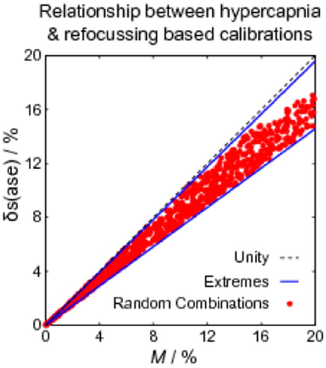
Simulations of M from hypercapnia calibration and δs(ase) from the ASE experiment. Each red marker represents a different combination of CBVt, Hct and OEF from the ranges detailed in the text. The relationship between δs(ase) and M appears to be mildly dependent on this physiological variability. The extremes of these physiological parameters are marked by blue lines. The gradients of these lines represent a prediction of the range of b_ase.

Methods

The goal of the experimental arm of this study was to empirically measure M using hypercapnia and estimate b_ase by comparing it with a measurement of δs(ase) acquired using an ASE experiment. Consistent with previous implementations of the calibrated BOLD approach in the literature (Hoge et al., 1999; Perthen et al., 2008; Bulte et al., 2009), these measurements were performed using ROI analysis. ROIs are typically functionally defined to minimise the inclusion of partial volumes of inactive tissue, whilst enabling spatial averaging of signals to increase the signal to noise ratio (SNR).

Imaging

A schematic diagram of the experimental protocol is provided by Fig. 2. Ethical approval was obtained from the local institutional review board. Eleven healthy subjects were recruited (6 male, 5 female) and informed consent to take part in the experiment was obtained. MR imaging was performed on a GE Signa HD× 3.0 T (GE Healthcare, Waukesha, WI) scanner equipped with an 8 channel parallel receive array coil and a body transmit coil. Single shot axial spiral images were acquired with a field of view of 256 mm, a matrix size of 64×64 and a foot-head slice coverage of 72 mm. Slices were positioned to cover a large fraction of the brain and the same slice coverage was used for both functional and calibration experiments. To correct for spatial blurring of the spirally acquired data caused by magnetic field inhomogeneity and the effects of through slice magnetic field gradients, two sets of FLASH images were acquired (Sutton et al., 2003). These images were collected with the same slice prescription as the functional scans using echo times (TE) of 3 ms and 5.5 ms and a repetition time (TR) of 1 s.

Figure 2.

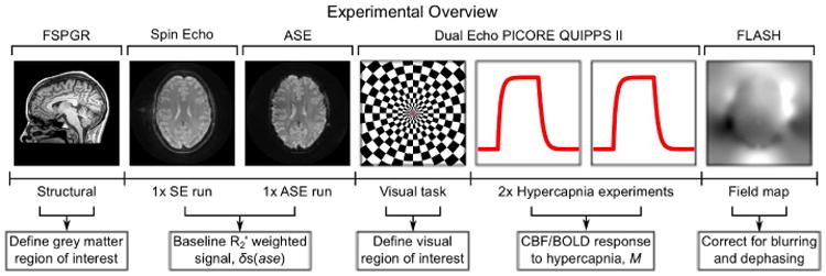
Overview of the experimental measurements made in this study and the purpose of each of the measurements.

Multi-shot spiral ASE/SE data (4 interleaves) were acquired with TR=3 s and TE=40 ms. ASE data were acquired with a τ of 30 ms. Images were acquired with a 128×128 matrix and 24 slices. Twenty-five repetitions were collected with the ASE and SE experiment.

For the hypercapnic calibration and functional experiments, dual echo arterial spin labelling (ASL) data were acquired. This consisted of a PICORE QUIPPSII labelling scheme (Wong et al., 1998) with TI₁=700 ms and TI₂=1750 ms. Two echoes were collected with TE₁=3.3 ms and TE₂=30 ms and a TR=3 s. Four images were discarded from each ASL data set to enable the MRI signal to reach a steady state.

A high resolution structural image was acquired for each subject using a 3D magnetisation prepared Fast SPoiled GRadient acquisition in the steady state (FSPGR) sequence (172 slices, 256×256 matrix, 1 mm isotropic resolution), which is a variant of MP-RAGE technique (Mugler and Brookeman, 1990).

Calibration Protocol and Stimulus Presentation

During each calibration scan subjects were instructed to fixate on a small stationary red square positioned centrally on a grey screen. This presentation was generated using the Psychophysics Toolbox (Brainard, 1997), projected through a wave guide and viewed via a mirror attached to the 8 channel receiver coil. Total experimental time for the ASE calibration was 10 minutes.

For the hypercapnic calibration, subjects breathed a 5% carbon dioxide, 21% oxygen, 74% nitrogen gas mixture from a previously filled reservoir connected to a non-rebreathing sequential gas delivery (SGD) circuit (Pulmanex Hi-Ox, Viasys Healthcare, Yorba Linda, CA, USA). The respiratory challenge was presented in an interleaved protocol of 2 min air, 3 min hypercapnia and 2 min air, with transitions achieved by manual switching. Due to a delay in the gas delivery system, the subject was switched to the hypercapnic gas mixture 30 s early, i.e. 1 min 30 s into the experiment. Each hypercapnia run lasted 7 min consisting of 210 repetitions, and was repeated twice for a total experimental duration of 14 min.

The functional stimulus consisted of a black and white radial checkerboard flickering at 8 Hz with a central red fixation square. The stimulus run consisted of four cycles of 60 s off and 20 s on, giving a scan duration of 6 min 20 s.

Throughout these experiments physiological monitoring data were recorded. This consisted of pulse, respiratory, and expiratory gas (O₂ and CO₂) waveforms, which were measured by a pulse oximeter, respiratory bellows and a mass spectrometer, respectively.

Pre-processing and Region of Interest Definition

Spiral data were initially corrected for spatial blurring caused by magnetic field ingomogeneity (Sutton et al., 2003). All images in the ASE and ASL datasets were corrected for subject motion, and registered to each subject's own structural scan, using AFNI software (Cox, 1996). CBF and BOLD weighted images were generated from the dual echo ASL data by performing an interpolated subtraction or addition, respectively. First echo data were used to measure changes in CBF, whilst second echo data were used to determine changes in the BOLD signal.

ROIs were defined in order to estimate M from hypercapnia calibration and δs(ase) from the ASE experiment. Firstly a functional ROI was defined from the visual stimulus experiment using a General Linear Model (GLM) analysis for ASL data (Mumford et al., 2006; Restom et al., 2006), incorporating image based correction for cardiac and respiratory physiological noise (Glover et al., 2000). Further analysis was confined to the occipital brain region defined by the MNI structural brain atlas (Mazziotta et al., 2001) transformed into functional space. Only voxels with a statistically significant CBF activation were included in the visual ROI, after correction for multiple comparisons at an overall significance threshold of p=0.05 using AFNI AlphaSim (Forman et al., 1995; Cox, 1996). Secondly a grey matter ROI was defined by segmenting the structural FSPGR data. Partial volume maps were generated from the structural images by first removing non-brain tissue using BET (Brain Extraction Tool) (Smith, 2002) and then performing automated segmentation using FAST (FMRIB's Automated Segmenation Tool) (Zhang et al., 2001). These maps were then transformed into functional space using FLIRT (FMRIB's Linear Image Registration Tool) (Jenkinson et al., 2002). The grey matter ROI was created by thresholding the resulting grey matter partial volume estimates at 75%.

Estimation of M and δs(ase)

Data were acquired from 11 subjects, but estimation of M and δs(ase) for the grey matter ROI was only possible in 9 subjects due to an operator error (incorrectly entered τ value) during the ASE acquisition in 2 subjects. A further 2 subjects were excluded from the visual ROI analysis due to a poor response to the visual task in one subject and a poor response to the hypercapnia challenge in the visual ROI of the other. The haemodynamic responses to hypercapnia were extracted as the ratio of CBF changes, and the percentage BOLD signal changes, with respect to their respective normocapnic baseline levels. The normocapnic baseline was calculated over a 90 s time period before the hypercapnic manipulation (window between 15 s and 105 s from experiment onset). The time period for the hypercapnic state was chosen to avoid transients and therefore to represent steady state signals (window between 195 s and 285 s from experiment onset). CBF and BOLD measures were averaged over the two hypercapnia challenge experiments and further averaged over the visual or grey matter ROIs. A single value of M for each ROI was then calculated using Eq. (6) and (7) and assuming α=0.2 and β=1.3.

The ASE calibration data underwent the following processing steps. Firstly the effect of macroscopic magnetic field inhomogeneity was removed. This does not affect the SE acquisition, but results in additional R₂′ weighting in the ASE data that is not physiological in origin. It manifests as attenuation of the ASE signal (F) and is a function of τ.

$$S(\mathit{\text{ASE}},\mathit{\text{base}})=S_0{e}^{-{\mathit{\text{TE}}}_{\mathit{\text{se}}}{R}_2}{e}^{-\tau R_2^{\prime }}F(\tau )$$ (13)

For a linear through-plane magnetic field gradient, under the assumption of a square slice profile, this attenuation factor can be described by a sinc function (Yablonskiy, 1998),

$$F(\tau )=\frac{sin(\mathrm{\Delta }\omega \tau /2)}{\mathrm{\Delta }\omega \tau /2},$$ (14)

where Δω = γG_zΔz is the frequency difference across the voxel, G_z is the magnetic field gradient, Δz is the slice thickness and γ is the gyromagnetic ratio for hydrogen. The field maps used for spatial deblurring of the spiral data were resampled to the same resolution as the ASE data, under the assumption that macroscopic field inhomogeneity varies smoothly in space. The first derivative of the field map in the z-direction, G_z, was calculated and used to estimate the local signal attenuation factor, F(τ), for the ASE images (τ=30 ms) using Eq. (14). Images of F(τ) were then used to correct the ASE images for through-slice dephasing only. Images were not corrected for in-plane magnetic field gradients, but were minimised by reducing the in-plane voxel dimensions to 2mm × 2mm (Young et al., 1988). The corrected ASE images and the SE images were then resampled to the spatial resolution of the hypercapnia challenge/functional data. Signals from the SE and ASE images were averaged over the visual and grey matter ROIs, and then used to calculate δs(ase) for each ROI.

Results

The visual ROI analysis was performed in 7 subjects. The group mean M was measured as 14.7% whilst δs(ase) was estimated as 11.1%. The standard deviation across the group were 7.0% and 1.7%, respectively. This difference in variance between the methods was found to be significant at p<0.01 using a two-sample F-test for equal variance. The scaling factor b_ase between M and δs(ase), when calculated on a subject by subject basis, was found to have a group mean of 0.88 with a standard deviation of 0.36.

Table 1 presents the results from the 9 subjects included in the grey matter ROI analysis. The group mean M was measured to be 10.2% with a group mean δs(ase) of 9.1% and standard deviations of 2.0% and 1.8%, respectively. This difference in variance is not significant. The group mean scaling factor was estimated as 0.93 with a standard deviation of 0.32. We do not present estimates of R₂′ in this work since these values will be intrinsically linked to the measurement technique applied in this study, as discussed earlier in the Theory section. However, R₂′ may be calculated from δs(ase) and Eq. (11), where τ=30ms.

Table 1.

Measurements of M and δs(ase) taken from the ROI based on the grey matter partial volume map thresholded at 75%. The scaling constant b_ase was estimated using Eq. (12).

Subject	M	δs(ase)	base
1	8.5	8.3	0.97
2	12.7	8.8	0.69
3	10.6	9.2	0.87
5	9.9	8.0	0.81
6	9.3	7.3	0.79
7	8.7	9.5	1.10
8	11.2	11.0	0.98
10	13.5	7.2	0.54
11	7.5	12.6	1.68
Mean	10.2	9.1	0.93
SD	2.0	1.8	0.32

Discussion

The calibrated BOLD method enables the BOLD response to be quantified in terms of changes in CMRO₂. This additional robustness makes it possible to account for intersubject differences in baseline physiology due to drugs (Perthen et al., 2008), disease (Ances et al., 2011) and ageing (Ances et al., 2009) that would otherwise confound the interpretation of the qualitative BOLD response. Despite these advantages the technique is rarely used outside of a relatively small number of specialist centres. Calibration using hypercapnia induces a sense of breathlessness in subjects, which may be a limiting factor in some applications. These experiments are also time consuming and the required equipment is not widely available. Therefore the possibility of calibrating the BOLD response without administering gases is highly appealing and may remove one of the barriers for some neuroscientific applications that may benefit from the calibrated approach.

In this study the potential of a refocussing based calibration was considered in the context of the existing hypercapnia based respiratory calibration and the theoretical ideal calibration. It was observed that, in effect, the Davis model provides a means to scale the measured BOLD response to a hypercapnia challenge in order to approximate the conditions of zero deoxyhaemoglobin present in the ideal calibration. Whilst hypercapnia calibration seeks to emulate the physical removal of all of the deoxyhaemoglobin, the aim of refocussing based calibration is to refocus the effect of deoxyhaemoglobin on the MR signal using a spin echo. However, it is not possible to refocus all of the effects that contribute to the BOLD signal and therefore the measured R₂′ weighted signal needs to be scaled to approximate the conditions in the ideal calibration. Simulations suggest an approximately linear scaling factor termed b_ase that is mildly dependent on variations in haematocrit and the resting oxygen extraction fraction. The range of b_ase given typical variations in these parameters is predicted to be 0.74 to 0.95. Experimental measurements of M using hypercapnia calibration and a practical R₂′ weighted signal based on an ASE experiment, δs(ase), were acquired. The value of b_ase was empirically determined to be 0.88 for a visual ROI and 0.93 for a grey matter ROI.

Potential of refocussing based calibration

Refocussing based calibration has several clear advantages over the hypercapnia approach. In this study the ASE experiment had a duration of 10 minutes while the ASL/BOLD hypercapnia experiment lasted 14 minutes in total. However, this neglects the additional time required to set up the gas delivery system for hypercapnia calibration, which is an important consideration. By eliminating this system, specialised gas equipment and knowledge are not required, potentially enabling wider implementation of the calibrated BOLD approach.

It is also possible that refocussing based calibration could provide more precise estimates of M. The variance in the measurements of M based on the grey matter ROI are comparable and insignificantly different (Table 1). However, over the smaller functionally defined visual ROI the variance in the hypercapnia method is significantly greater than the ASE approach. Potentially this could allow calibration to be performed more reliably at the individual subject level rather than relying on group M values.

Comparison with earlier work

R₂′ has previously been exploited to measure CMRO₂ changes at 9.4 T in animals (Hyder et al., 2001) and 1.5 T in humans (Fujita et al., 2006). Both methods used a variant of the calibrated BOLD technique whereby the measured relaxation rates at rest and during activation are used directly in the estimation of changes in CMRO₂. In contrast our proposal follows the conventional calibrated BOLD approach by calculating M from a measurement of R₂′ and measuring the percentage change in the gradient echo BOLD signal.

A multi-shot spiral ASE sequence was used to measure R₂′ in this study. The experiments of (Fujita et al., 2006) used the Gradient Echo Sampling of FID and Echo (GESFIDE) (Ma and Wehrli, 1996) method and in the work of (Hyder et al., 2001) R₂ and R₂* were measured using separate pulse sequences with R₂′ calculated as the difference between these measures. One practical difficulty of the GESFIDE sequence is that the R₂ and R₂′ weighting of the acquired images varies simultaneously due to differing TE and τ for each image. Separation of these effects is difficult as both processes are exponential and is further complicated by the multiexponential behaviour of R₂ (Bottomley et al., 1984), often requiring R₂ to be measured in a separate experiment. In the ASE technique the R₂′ weighting of the image is manipulated independently of the R₂ weighted component of the signal. Since the R₂ weighted component remains constant the multiexponential behaviour of R₂ does not need to be corrected, simplifying the analysis. However, the variety of techniques that are available for the measurement of R₂′ serves to underline the importance of estimating an appropriate scale factor, b, for the particular technique that is used. It must be remembered that measurements of R₂′ should not be thought of as being independent of the technique with which they are measured. The multiexponential nature of the signal decay introduces a dependence on the specific parameters of the pulse sequence. This is particularly true of the parameters used in this study (see below).

The previously cited studies used a combination of high resolution image acquisition and post-processing to minimise the effect of macroscopic magnetic field inhomogeneity. A similar approach was followed in this study. To reduce the frequency difference across the voxel, due to magnetic field inhomogeneity, the voxel dimensions were reduced from 4×4×6 mm³ in the functional data to 2×2×3 mm³ for the ASE data (Young et al., 1988). As a further step a separately acquired magnetic field map was used to correct for through-slice dephasing only. A similar approach has previously been used in R₂* mapping (Fernández-Seara and Wehrli, 2000), but would require data with multiple τ values to implement in this experiment. Whilst magnetic field gradients in the through-slice direction are likely to account for the majority of signal loss, similar effects are expected to occur in plane. Corrections for these effects has previously been achieved by altering the acquisition method (Deichmann et al., 2002) or post-processing the data (Yablonskiy et al., 2013).

The simplest R₂′ weighted signal was generated by acquiring a spin echo and an asymmetric spin echo with a τ of 30ms. This is a potential disadvantage as the R₂′ signal decay is known to have two regimes: the short τ regime, where signal decay is quadratically exponential, and the long τ regime where it is linearly exponential (Yablonskiy and Haacke, 1994). By choosing a value of τ from both regimes the relationship between deoxyhaemoglobin concentration and the measured signal may become non-linear. The simulations in this work explicitly model this.

Limitations of the current study

The main limitation for applying the calibration described in this study is related to the scaling factor b_ase. Specifically this scale factor is only accurate for the ASE based experiment described here and not more generally for similar R₂′ weighted or relaxometry methods. It is likely that more accurate or reliable acquisition strategies are possible, but in this case the scaling factor must be measured, or otherwise estimated, for that specific experiment.

Predictions of the scaling factor from simulations are based on assuming a single tissue type: grey matter. In practice signal contamination from adjacent cerebral spinal fluid (CSF) or white matter is possible (He and Yablonskiy, 2007). We also assume that susceptibility is dominated by paramagnetic deoxyhaemoglobin. Care must be taken in iron or myelin rich regions of the brain due to the possibility of systematic error. Further work is required to better characterise their effect on R₂′.

Similarly the prediction of a linear scale factor between M and the measured R₂′ weighted signal could potentially be improved. We note some influence of intersubject variations in haematocrit and the oxygen extraction fraction. A more sophisticated model of b_ase could help reduce this influence. This would require more accurate simulations of the R₂′ weighted signal and a better understanding of the physiology and partial volume effects.

Conclusions

The feasibility of measuring the calibrated BOLD scaling parameter M using a refocussing based calibration was investigated. It was determined that, in a similar manner to hypercapnia calibration, the measured R₂′ weighted signal must be scaled to determine M. This scale factor was empirically determined with reference to hypercapnia calibration. These experiments have shown that refocussing based calibration is a promising approach for greatly simplifying the calibrated BOLD methodology by eliminating the need for the subject to breathe special gas mixtures, and potentially provides the basis for a wider implementation of quantitative fMRI.

Highlights.

The feasibility of calibrated BOLD without gas administration was investigated.

The BOLD scaling parameter M was measured using a refocussing based calibration.

Similar to hypercapnia calibration, a scale factor is required to estimate M.

The scale factor was predicted by simulations to be approximately linear.

The scale factor was empirically measured with reference to hypercapnia calibration.

References

- Ances BM, Liang CL, Leontiev O, Perthen JE, Fleisher AS, Lansing AE, Buxton RB. Effects of aging on cerebral blood flow, oxygen metabolism, and blood oxygenation level dependent responses to visual stimulation. Hum Brain Mapp. 2009;30:1120–1132. doi: 10.1002/hbm.20574. [DOI] [PMC free article] [PubMed] [Google Scholar]
- Ances BM, Vaida F, Ellis R, Buxton RB. Test-retest stability of calibrated BOLD-fMRI in HIV- and HIV+ subjects. Neuroimage. 2011;54:2156–2162. doi: 10.1016/j.neuroimage.2010.09.081. [DOI] [PMC free article] [PubMed] [Google Scholar]
- Blockley N, Griffeth VEM, Buxton RB. A general analysis of calibrated BOLD methodology for measuring CMRO2 responses: Comparison of a new approach with existing methods. Neuroimage. 2012;60:279–289. doi: 10.1016/j.neuroimage.2011.11.081. [DOI] [PMC free article] [PubMed] [Google Scholar]
- Blockley N, Griffeth VEM, Simon AB, Buxton RB. A review of calibrated blood oxygenation level-dependent (BOLD) methods for the measurement of task-induced changes in brain oxygen metabolism. NMR Biomed. 2013;26:987–1003. doi: 10.1002/nbm.2847. [DOI] [PMC free article] [PubMed] [Google Scholar]
- Bottomley PA, Foster TH, Argersinger RE, Pfeifer LM. A review of normal tissue hydrogen NMR relaxation times and relaxation mechanisms from 1-100 MHz: dependence on tissue type, NMR frequency, temperature, species, excision, and age. Med Phys. 1984;11:425–448. doi: 10.1118/1.595535. [DOI] [PubMed] [Google Scholar]
- Boxerman JL, Hamberg LM, Rosen BR, Weisskoff RM. MR contrast due to intravascular magnetic susceptibility perturbations. Magn Reson Med. 1995;34:555–566. doi: 10.1002/mrm.1910340412. [DOI] [PubMed] [Google Scholar]
- Brainard DH. The Psychophysics Toolbox. Spat Vis. 1997;10:433–436. [PubMed] [Google Scholar]
- Bulte DP, Drescher K, Jezzard P. Comparison of hypercapnia-based calibration techniques for measurement of cerebral oxygen metabolism with MRI. Magn Reson Med. 2009;61:391–398. doi: 10.1002/mrm.21862. [DOI] [PubMed] [Google Scholar]
- Cox RW. AFNI: software for analysis and visualization of functional magnetic resonance neuroimages. Comput Biomed Res. 1996;29:162–173. doi: 10.1006/cbmr.1996.0014. [DOI] [PubMed] [Google Scholar]
- Davis TL, Kwong KK, Weisskoff RM, Rosen BR. Calibrated functional MRI: mapping the dynamics of oxidative metabolism. Proc Natl Acad Sci USA. 1998;95:1834–1839. doi: 10.1073/pnas.95.4.1834. [DOI] [PMC free article] [PubMed] [Google Scholar]
- Deichmann R, Josephs O, Hutton C, Corfield DR, Turner R. Compensation of susceptibility-induced BOLD sensitivity losses in echo-planar fMRI imaging. Neuroimage. 2002;15:120–135. doi: 10.1006/nimg.2001.0985. [DOI] [PubMed] [Google Scholar]
- Fernández-Seara MA, Wehrli FW. Postprocessing technique to correct for background gradients in image-based R*(2) measurements. Magn Reson Med. 2000;44:358–366. doi: 10.1002/1522-2594(200009)44:3<358::aid-mrm3>3.0.co;2-i. [DOI] [PubMed] [Google Scholar]
- Forman SD, Cohen JD, Fitzgerald M, Eddy WF, Mintun MA, Noll DC. Improved assessment of significant activation in functional magnetic resonance imaging (fMRI): use of a cluster-size threshold. Magn Reson Med. 1995;33:636–647. doi: 10.1002/mrm.1910330508. [DOI] [PubMed] [Google Scholar]
- Fujita N, Matsumoto K, Tanaka H, Watanabe Y, Murase K. Quantitative study of changes in oxidative metabolism during visual stimulation using absolute relaxation rates. NMR Biomed. 2006;19:60–68. doi: 10.1002/nbm.1001. [DOI] [PubMed] [Google Scholar]
- Glover GH, Li TQ, Ress D. Image-based method for retrospective correction of physiological motion effects in fMRI: RETROICOR. Magn Reson Med. 2000;44:162–167. doi: 10.1002/1522-2594(200007)44:1<162::aid-mrm23>3.0.co;2-e. [DOI] [PubMed] [Google Scholar]
- Griffeth VEM, Buxton RB. A theoretical framework for estimating cerebral oxygen metabolism changes using the calibrated-BOLD method: Modeling the effects of blood volume distribution, hematocrit, oxygen extraction fraction, and tissue signal properties on the BOLD signal. Neuroimage. 2011;58:198–212. doi: 10.1016/j.neuroimage.2011.05.077. [DOI] [PMC free article] [PubMed] [Google Scholar]
- He X, Yablonskiy DA. Quantitative BOLD: Mapping of human cerebral deoxygenated blood volume and oxygen extraction fraction: Default state. Magn Reson Med. 2007;57:115–126. doi: 10.1002/mrm.21108. [DOI] [PMC free article] [PubMed] [Google Scholar]
- Hoge RD, Atkinson J, Gill B, Crelier GR, Marrett S, Pike GB. Investigation of BOLD signal dependence on cerebral blood flow and oxygen consumption: the deoxyhemoglobin dilution model. Magn Reson Med. 1999;42:849–863. doi: 10.1002/(sici)1522-2594(199911)42:5<849::aid-mrm4>3.0.co;2-z. [DOI] [PubMed] [Google Scholar]
- Hyder F, Kida I, Behar KL, Kennan RP, Maciejewski PK, Rothman DL. Quantitative functional imaging of the brain: towards mapping neuronal activity by BOLD fMRI. NMR Biomed. 2001;14:413–431. doi: 10.1002/nbm.733. [DOI] [PubMed] [Google Scholar]
- Jenkinson M, Bannister P, Brady M, Smith S. Improved optimization for the robust and accurate linear registration and motion correction of brain images. Neuroimage. 2002;17:825–841. doi: 10.1016/s1053-8119(02)91132-8. [DOI] [PubMed] [Google Scholar]
- Ma J, Wehrli FW. Method for image-based measurement of the reversible and irreversible contribution to the transverse-relaxation rate. J Magn Reson B. 1996;111:61–69. doi: 10.1006/jmrb.1996.0060. [DOI] [PubMed] [Google Scholar]
- Mazziotta J, Toga A, Evans A, Fox P, Lancaster J, Zilles K, Woods R, Paus T, Simpson G, Pike B, Holmes C, Collins L, Thompson P, MacDonald D, Iacoboni M, Schormann T, Amunts K, Palomero-Gallagher N, Geyer S, Parsons L, Narr K, Kabani N, Le Goualher G, Boomsma D, Cannon T, Kawashima R, Mazoyer B. A probabilistic atlas and reference system for the human brain: International Consortium for Brain Mapping (ICBM) Philos Trans R Soc Lond, B, Biol Sci. 2001;356:1293–1322. doi: 10.1098/rstb.2001.0915. [DOI] [PMC free article] [PubMed] [Google Scholar]
- Mugler JP, Brookeman JR. Three-dimensional magnetization-prepared rapid gradient-echo imaging (3D MP RAGE) Magn Reson Med. 1990;15:152–157. doi: 10.1002/mrm.1910150117. [DOI] [PubMed] [Google Scholar]
- Mumford JA, Hernandez-Garcia L, Lee GR, Nichols TE. Estimation efficiency and statistical power in arterial spin labeling fMRI. Neuroimage. 2006;33:103–114. doi: 10.1016/j.neuroimage.2006.05.040. [DOI] [PMC free article] [PubMed] [Google Scholar]
- Perthen JE, Lansing AE, Liau J, Liu TT, Buxton RB. Caffeine-induced uncoupling of cerebral blood flow and oxygen metabolism: a calibrated BOLD fMRI study. Neuroimage. 2008;40:237–247. doi: 10.1016/j.neuroimage.2007.10.049. [DOI] [PMC free article] [PubMed] [Google Scholar]
- Restom K, Behzadi Y, Liu TT. Physiological noise reduction for arterial spin labeling functional MRI. Neuroimage. 2006;31:1104–1115. doi: 10.1016/j.neuroimage.2006.01.026. [DOI] [PubMed] [Google Scholar]
- Smith SM. Fast robust automated brain extraction. Hum Brain Mapp. 2002;17:143–155. doi: 10.1002/hbm.10062. [DOI] [PMC free article] [PubMed] [Google Scholar]
- Sutton BP, Noll DC, Fessler JA. Fast, iterative image reconstruction for MRI in the presence of field inhomogeneities. IEEE Trans Med Imaging. 2003;22:178–188. doi: 10.1109/tmi.2002.808360. [DOI] [PubMed] [Google Scholar]
- Wismer GL, Buxton RB, Rosen BR, Fisel CR, Oot RF, Brady TJ, Davis KR. Susceptibility induced MR line broadening: applications to brain iron mapping. J Comput Assist Tomogr. 1988;12:259–265. doi: 10.1097/00004728-198803000-00014. [DOI] [PubMed] [Google Scholar]
- Wong EC, Buxton RB, Frank LR. Quantitative imaging of perfusion using a single subtraction (QUIPSS and QUIPSS II) Magn Reson Med. 1998;39:702–708. doi: 10.1002/mrm.1910390506. [DOI] [PubMed] [Google Scholar]
- Yablonskiy DA. Quantitation of intrinsic magnetic susceptibility-related effects in a tissue matrix. Phantom study. Magn Reson Med. 1998;39:417–428. doi: 10.1002/mrm.1910390312. [DOI] [PubMed] [Google Scholar]
- Yablonskiy DA, Haacke EM. Theory of NMR signal behavior in magnetically inhomogeneous tissues: the static dephasing regime. Magn Reson Med. 1994;32:749–763. doi: 10.1002/mrm.1910320610. [DOI] [PubMed] [Google Scholar]
- Yablonskiy DA, Sukstanskii AL, Luo J, Wang X. Voxel spread function method for correction of magnetic field inhomogeneity effects in quantitative gradient-echo-based MRI. Magn Reson Med. 2013;70:1283–1292. doi: 10.1002/mrm.24585. [DOI] [PMC free article] [PubMed] [Google Scholar]
- Young IR, Cox IJ, Bryant DJ, Bydder GM. The benefits of increasing spatial resolution as a means of reducing artifacts due to field inhomogeneities. Magn Reson Imaging. 1988;6:585–590. doi: 10.1016/0730-725x(88)90133-6. [DOI] [PubMed] [Google Scholar]
- Zhang Y, Brady M, Smith S. Segmentation of brain MR images through a hidden Markov random field model and the expectation-maximization algorithm. IEEE Trans Med Imaging. 2001;20:45–57. doi: 10.1109/42.906424. [DOI] [PubMed] [Google Scholar]