Sonic Estimation of Elasticity via Resonance: A New Method of Assessing Hemostasis

Abstract

Uncontrolled bleeding threatens patients undergoing major surgery and in care for traumatic injury. This paper describes a novel method of diagnosing coagulation dysfunction by repeatedly measuring the shear modulus of a blood sample as it clots in vitro. Each measurement applies a high-energy ultrasound pulse to induce a shear wave within a rigid walled chamber, and then uses low energy ultrasound pulses to measure displacements associated with the resonance of that shear wave. Measured displacements are correlated with predictions from Finite Difference Time Domain (FDTD) models, with the best fit corresponding to the modulus estimate. In our current implementation each measurement requires 62.4 ms. Experimental data was analyzed using a fixed-viscosity algorithm and a free-viscosity algorithm. In experiments utilizing human blood induced to clot by exposure to kaolin, the free-viscosity algorithm quantified the shear modulus of formed clots with a worst-case precision of 2.5%. Precision was improved to 1.8% by utilizing the fixed-viscosity algorithm. Repeated measurements showed a smooth evolution from liquid blood to a firm clot with a shear modulus between 1.4 kPa and 3.3 kPa. These results show the promise of this technique for rapid, point of care assessment of coagulation.

Introduction

Hemostasis is the physiological process that stops bleeding. Functional hemostasis requires the balanced engagement of plasma coagulation factors to initiate clotting, adequate fibrinogen to form the fibrin mesh, platelets to modulate factor function and to mechanically stiffen the mesh, and fibrinolytic enzymes to eliminate the clot when it is no longer needed (1). Perturbation of any of these subsystems can disrupt hemostasis either by interfering with clotting or by initiating clotting when it is unneeded. Disruptions of hemostasis contribute to morbidity and mortality in patients suffering from heart disease (2), stroke (3), traumatic injury (4), cancer (5), and sepsis (6).

While hemostatic dysfunction impacts a broad range of medical conditions, it has been studied intensively in cardiac surgery. Cardiac bypass is associated with significant post-operative bleeding. This is caused by platelet damage by the bypass pump, factor and fibrinogen consumption associated with surgical trauma, and the occasional presence of residual anti-coagulant. A number of strategies are currently used to manage this dysfunction. The least informed and most widely used strategy is a “shotgun therapy” approach; blindly transfusing varying combinations of fresh frozen plasma, cryoprecipitate or fibrinogen concentrate, and platelet concentrate. This approach is often successful in controlling bleeding, however unnecessary transfusion carries a significant financial cost and increases patient morbidity and mortality (7,8). Recognition of the risks associated with excessive transfusion have led to increasingly specific and detailed guidelines to manage transfusion (9). These guidelines call for transfusion to be “guided by point-of-care tests that assess hemostatic function in a timely and accurate manner.” No currently available product combines the ease of use, rapid turnaround time, and robust performance needed to fully satisfy this clinical need.

A number of approaches have been proposed for point-of-care hemostasis testing. These technologies can be separated into broad categories: clot-time assays, platelet-only tests, and viscoelastic tests. Clot-time assays can be implemented with simple technology, however clot time alone offers only limited clinical insight. Consider a patient with severe fibrinogen deficiency. This patient may clot rapidly, but that clot will be too mechanically weak to stop bleeding. Furthermore, clot-time assays generally operate on plasma, rather than whole blood, and therefore neglect the important interactions between plasma coagulation factors and platelets. Platelet-only tests provide useful information, but are also limited in that they also neglect interactions between platelets and plasma coagulation factors. Both clot-time assays and platelet-only tests are typically conducted in core or satellite laboratories at some distance from the patient. Transporting the sample to the laboratory and then communicating results back to the treating clinician can require an hour or more, significantly delaying treatment. Unlike clot-time and platelet-only tests, viscoelastic tests have been shown to provide broadly useful clinical information (10). Nonetheless, these instruments have found limited clinical application because they require significant training to use and interpret, they are not well suited to point of care testing, and their test times are considered too slow by many clinicians.

Clinically available viscoelastic tests include the Thromboelastogram (TEG), Rotational Thromboelastometer (ROTEM), Sonoclot, and ReoRox. The TEG is a concentric cylinder rheometer. A blood sample is mixed with reagents by a manual pipette and 360 μl of the mixture is added to a test cup. A motor rotates the cup while an optical sensor measures the rotation of an immersed pin suspended on a torsion wire. The TEG has been widely studied and has been shown to provide valuable information in numerous clinical settings (10). The ROTEM (Rotational Thromboelastometer) operates on a similar principle, with the cup being fixed and the pin rotating and measuring strain. The Sonoclot uses a piston oscillating along its major axis to measure clot viscoelasticity. The Sonoclot is limited in that the clot tends to pull away from the piston as it reaches maximum stiffness; making measurement at peak stiffness impossible (10). The ReoRox utilizes a cup and pin geometry, but rather than using a continuous oscillating drive, it rotates the cup, holds it for one second, and then releases it. The cup then oscillates and the system measures the modulus from the oscillation frequency and the viscosity from the rate of decay of oscillation. The ReoRox is the only currently available instrument able to quantify the viscosity of both the liquid blood and the formed clot (32).

In addition to direct mechanical tests, a number of ultrasound-based viscoelastic tests have been described. We have previous described sonorheometry, a method that applies ultrasound radiation force and measures the resultant displacement to infer stiffness (11-13). Sonorheometry utilizes relatively small blood volumes (< 1ml), however quantitative measurement requires the knowledge of the applied radiation force magnitude, which is difficult to know in practice.

A number of groups have proposed the measurement of shear wave velocity to quantify sample modulus. Velocity can be measured between laterally separated points (14), axially separated points (15), or throughout a field via imaging (16). These methods have the advantage of being fundamentally quantitative, however the need to measure displacements at two separated points requires a significant blood sample volume. Schmitt et al used a 60 ml sample, for example. Such large volumes are not practical for human diagnostics.

In this work we describe Sonic Estimation of Elasticity via Resonance (SEER), a novel modulus estimation technique designed for in vitro applications. SEER Sonorheometry builds upon our prior method, sonorheometry, by enabling quantitative modulus measurement. SEER applies acoustic radiation force to induce shear wave resonance within a rigid test chamber and compares the characteristics of that resonance to numerical or analytical models to quantify the shear modulus of the sample filling the chamber. This work describes the SEER method and the Finite Difference Time Domain model from which we estimate modulus. We present experimental results performed using prototype test cartridges in multiple prototype Quantra^™ instruments. These experiments show that SEER measurements exhibit low noise and high precision. We derive bounds on SEER performance and describe plans for future refinement.

Materials and Methods

SEER: Sonic Estimation of Elasticity via Resonance

SEER consists of three interconnected steps: data acquisition, motion estimation, and modulus estimation. SEER is shown schematically in Fig. 1. Data acquisition begins as a low energy sensing pulse is transmitted into a rigid test chamber filled with the sample under test. In Fig. 1 this pulse travels from left to right along the region indicated by the vertical lines within the test chamber. This sensing pulse returns a reference echo indicating the positions of acoustic scatterers within the sample prior to the application of significant radiation force. In human blood the acoustic scatterers consist almost entirely of red blood cells (17). Next a high intensity forcing pulse is transmitted into the sample to apply acoustic radiation force (18). This force displaces the sample along the ultrasound beam axis in the direction of ultrasound propagation. This displacement induces a propagating shear wave that travels outward from the ultrasound beam in a direction perpendicular to the ultrasound wave propagation (19). This shear wave is shown as the shaded regions in Fig. 1. Finally, a series of low intensity sensing pulses are transmitted. Each sensing pulse returns an echo from the beam axis that incorporates the movement associated with the propagating shear wave. We refer to the collection of a force transmission and associated sensing transmissions as an ensemble.

Figure 1.

Schematic representation of the SEER method. SEER begins with data acquisition, during which a high intensity ultrasound pulse applies acoustic radiation force to induce a shear wave that resonates within the test chamber. A series of low energy sensing pulses are used to acquire ultrasound echoes from the moving sample. These echoes are processed to form motion estimates indicative of the resonating shear wave. Equations in the ‘Motion Estimation’ panel explain how time-delay estimates are converted into displacements estimates. Motion estimates are compared to numerical or analytical models to find the shear modulus (and possibly other mechanical properties) that best fits the observed motion. This process is repeated every few seconds to measure the evolving shear modulus resulting from coagulation.

The echoes acquired during the data acquisition phase are processed in the motion estimation phase. Motion estimation can be performed using a number of well-known algorithms, with various tradeoffs between variance, bias, and computational complexity (20). In this paper we use the motion estimation algorithm described in (21), subject to proprietary modifications. This stage of SEER yields a time-displacement curve indicative of the shear wave induced axial motion along the ultrasound beam.

In SEER’s final stage we analyze the experimental time-displacement curve to estimate the shear modulus of the sample. This analysis can follow at least two distinct paths: comparison with a numerical model or comparison with an analytical model. Comparison with an analytical model can take the form of matching signal shape or specific signal characteristics such as resonant frequency. In this paper we focus entirely on comparison with a numerical model. This is preferred because the complex geometry of our resonant test chamber makes analytical modeling extremely challenging. In contrast, numerical modeling is straightforward, even for complex geometries. Our numerical models use an axisymmetric Finite Different Time Domain (FDTD) model. This approach is advantageous because it can be implemented easily in MATLAB, execution time is rapid enough that we can build a large library of results, and it is flexible enough that we can capture the relevant geometry of the experimental test chamber. The axisymmetric FDTD model is derived in Appendix A.

In the modulus estimation phase we compare the experimental time-displacement curve to a library of numerically determined time-displacement curves. This comparison is performed efficiently via normalized correlation, as described in Eq. 1:

$${\rho }_{\mathit{Nd}}=\mathbf{N}{\left(\frac{1}{\sqrt{e_d}}(\widehat{\mathit{d}}-a_d-b_d\mathit{t})\right)}^{\mathit{T}}$$ (1)

Where ρ_Nd is a column vector of normalized correlation coefficients, $\widehat{\mathit{d}}$ is a row vector of estimated displacements, a_d is the mean of $\widehat{\mathit{d}}$, b_d is the slope of the best fit line through the displacements $\widehat{\mathit{d}}$, and e_d is the energy (sum squared value) of the displacements after removal of the mean and linear trend, t is a vector of the times at which the displacements were estimated, and N is a matrix with each row vector consisting of a processed FDTD model output. Each row vector in N is equal to:

$${\mathit{n}}_{\mathit{j}}=\frac{1}{\sqrt{e_{n_j}}}\left({\mathit{d}}_{\mathit{j}}-a_{n_j}-b_{n_j}\mathit{t}\right)$$ (2)

where d_j is the unprocessed time-displacement estimate from the FDTD model and the other terms are analogous to those of Eq. 1. By pre-processing the model output and experimental time-displacements, the normalized correlations are computed using a single matrix multiply. The computation of the correlation coefficient described by Eq. 1 requires less than 4.0ms in MATLAB on a high-end laptop for a 16,032 × 512 free-viscosity model.

The formal definition of the normalized correlation requires removal of neither the signal mean nor its linear trend. These additional steps are informed by observed characteristics in the experimental time-displacement data. We expect the measured time-displacement curve to be a zero mean signal, at least for cases where the observation time is significantly longer than the time constant of the damped response. Contrary to this expectation, we observe that experimental time-displacement curves have a linear trend and signal offset (after the first displacement estimate) that varies from one acquisition to the next. The offset appears to be a result of reverberation, as the pre-force sensing echo is somewhat decorrelated from the post-force echoes. We believe that the linear trend is the result of the accumulation of small displacements induced by the sensing pulses and speed of sound changes resulting from acoustic heating within the acoustic path. Regardless of the source, we have found that removal of offsets and linear trends yields more precise and consistent measurements.

In addition to removing the offset and linear trend of the time-displacements, we remove the first few time-displacement estimates prior to computing the correlation. We observe that the forcing pulse introduces significant reverberation into the received signals and thereby corrupts the early time-displacement estimates. The number of estimates trimmed is somewhat arbitrary, but in the results presented below we trim the first 18 time-displacement estimates from an ensemble of 512. This step is performed before removal of the mean and linear trend.

The precision and accuracy of SEER depends fundamentally upon the quality of the model to which the experimental data is correlated. To explore this relationship we considered two specific models. The first was a free-viscosity model in which we allowed both the shear viscosity and the shear modulus to vary. The second approach used a fixed-viscosity model in which the shear viscosity was held constant while the shear modulus was allowed to vary. We expect the free-viscosity model to exhibit a lower bias because of its ability to fit arbitrary or even changing viscosities. This will come at the cost of increased variance. These two models effectively explore the impact of viscosity on the bias and variance of estimated modulus. Specific FDTD implementation details are described in Table 1.

Table 1.

Experimental Acquisition parameters.

Acquisition Parameter	Value
Shared
Pulse Repetition Frequency	8,206.4 Hz
Ensemble Definition	1 sense, 1 force, 511 sense
Ensemble Length	62.4 ms
Ensemble Interval	4 or 6 seconds
Transmit Subsystem
Sampling Rate	125 MHz
Receive Subsystem
ADC Precision	12 bits
Sampling Rate	62.5 MHz
Processed Window Length	96 samples / 1.536 μs / 1.23 mm @ 1600 m/s
Sensing Pulse
Center Frequency	6.94 MHz
Pulse Duration	1 cycle / 144 ns
Forcing Pulse
Center Frequency	5.21 MHz
Pulse Duration	75 cycles / 14.4 μs

The shear modulus can be estimated directly by finding the peak of the normalized correlation vector computed in Eq. 1. While such an approach is straightforward, it yields quantization artifacts because of the relatively crude sampling of modulus in the FDTD model. To overcome this limitation we find the analytical location of the peak of an interpolated correlation function. Interpolation of the fixed-viscosity model is straightforward. We simply locate the peak discrete correlation value and its two nearest neighbors, fit a parabola to these points, and then locate the peak of this analytical function. The location of the peak of the parabola is the estimated modulus. For the free-viscosity model interpolation is more complicated. In this case we locate the largest correlation coefficient, its four nearest neighbors (north, south, east, and west), and select one correlation value at a diagonal (such as north-east). To these six data points we fit an arbitrary two-dimensional quadratic curve, as described in Eq. 3. We locate the peak of this function analytically to estimate the modulus (μ) and viscosity (η) of the sample.

$$R(\mu ,\eta )=g_1+g_2\mu +g_3\eta +g_4\mu \eta +g_5{\mu }^2+g_6{\eta }^2$$ (3)

Each ensemble yields a single modulus or modulus / viscosity estimate. Ensembles are repeated to measure dynamic changes in modulus associated with clotting. The maximal ensemble rate is determined by the intrinsic ensemble acquisition time and the relaxation time of the sample.

Instrumentation

All experiments were performed using prototype Quantra^™ systems with prototype four-channel test cartridges. A design rendering of the current four-channel test cartridge is shown in Fig. 2. The Quantra^™ system incorporates an embedded computer, a touchscreen user interface, four independently controlled cartridge heaters, pneumatic valves, optical sensors for control feedback, and a peristaltic pump to control sample flow through the cartridge. Ultrasound acquisition is performed using four single element unfocused transducers and custom circuitry. System heaters were held at 37°C for all experiments. At the time of writing this paper all data analysis was performed offline.

Figure 2.

Prototype Quantra^™ cartridge. This four-channel cartridge incorporates a warming chamber, volume control chambers to set sample volume, liquid reagents, and four independent test chambers. Ultrasound is coupled in from the opposite face.

The prototype test cartridge includes chambers for sample warming, sample volume control, liquid reagents, and SEER measurement. Blood is initially drawn into the warming chamber and held to ensure a precise test temperature of 37°C. Next the blood is drawn into the volume control chambers to ensure that each test channel receives closely matched blood volumes. The blood sample and liquid reagents are mixed by repeated cyclic flow through the visible serpentine channels. The inner surfaces of the measurement chambers were plasma treated to enhance clot adhesion. Each test chamber incorporates a compressible elastomer couplant and acoustic lens. A complete four-channel test requires approximately 1.7ml of blood, with each measurement chamber requiring roughly 300 μl.

Ultrasound data acquisition was performed following the parameters in Table 1. The Pulse Repetition Frequency (PRF) was selected to yield the maximum temporal sampling rate that did not result in excessive reverb within the test volume. The processed window length was selected to capture the largest spatial window over which the SEER signal was statistically stationary, while also avoiding ranges with significant fixed reverberation. The ensemble length was the maximum achievable for the finite memory of the Field Programmable Gate Array we used for data acquisition. The forcing pulse center frequency was selected empirically to maximize displacement. This frequency was likely optimal because it offered the best impedance match between the transducer and transmitter. Improvements in impedance matching will likely allow the use of higher frequency forcing pulses that should increase displacement due to higher scattering and absorption at higher frequency. The forcing pulse length is somewhat arbitrary. The sensing pulse frequency was selected empirically to achieve low reverberation, high echo sensitivity, and low jitter in time-displacement estimates. A single cycle sensing pulse was utilized to maximize echo bandwidth.

The geometry of the acoustic path, acoustic beams, and test chamber are shown in Fig. 3. Ultrasound waves are emitted by the transducer and pass through a rigid standoff. An elastomeric couplant, incorporated into the test cartridge, is compressed against the standoff to provide ultrasound coupling between the instrument and cartridge. The curved geometry of the elastomer / cartridge body interface acts as an acoustic lens with a focus near the back of the test chamber. Acoustic radiation force applied by the forcing beam displaces the clot along the beam axis and away from the transducer. The field of induced axial displacement propagates radially away from the forcing beam as a shear wave. The sensing beam detects axial motion as the shear wave reverberates within the test chamber.

Figure 3.

Acoustic path and test chamber geometry with overlaid sensing beam (left) and forcing beam (right). The displayed sensing beam is the square of the two-way sensitivity function. The displayed forcing beam is the energy of transmitted forcing beam. Ultrasound beams were modeled using FIELD II (29) with acoustic properties for blood taken from (30).

Finite Difference Time Domain Models

Finite Difference Time Domain models and subsequent data analysis were implemented in Matlab R2014b (The Mathworks, Natick, MA). The FDTD model is derived in detail in Appendix A.

FDTD models were built to mimic the geometry of the prototype Quantra^™ test cartridge. The geometry of the test well and the FDTD model are shown in Fig. 4. The FDTD model geometry closely matches that of the test chamber, although the modeled conical region is axisymmetric, unlike the actual cartridge. The model geometry is inconsistent with the cartridge in other minor ways. Although we do not believe that these discrepancies will have significant impact, we intend to correct them in future work. All walls of the FDTD model were completely rigid, except the base of the conical region, which consisted of a 20 sample absorbing boundary layer (not shown in the diagram). The absorbing boundary was implemented following (22), with identical parameters except for thickness (i.e. m = 2.1 and τ_max = 0.1). The perfectly rigid walls were implemented by setting the velocities within the walls equal to zero in each iteration. Additional details of the FDTD model implementation are described in Table 2.

Figure 4.

Experimental test chamber geometry (left) and FDTD model geometry (right). Gray regions indicate the full width at half maximum of the modeled ultrasound forcing beam. All dimensions are in mm.

Table 2.

FDTD Model Parameters.

Model Parameter	Value
Shared
Spatial Sampling Interval	100 μm
Temporal Sampling Rate	393,216 Hz
Blood Density	1060 kg/m3
Free-viscosity Model
Shear Viscosity	32 values from 0.001 to 0.8 Pa s
Shear Modulus	501 values from 10 to 10,000 Pa
Fixed-viscosity Model
Shear Viscosity	1 value of 0.25 Pa s
Shear Modulus	1,167 values from 0.001 to 10,000 Pa
Force Function
Center	8.78 mm from test chamber base
Full Width at Half Maximum in range	5.90 mm
Full Width at Half Maximum in azimuth	660 μm

Radiation force was applied in a single time sample at the beginning of the simulation. The force field was modeled as a Gaussian function defined by the parameters in Table 2. The focal depth and beam geometry were selected to match an ultrasound beam measurement performed with an earlier, similar lens design. This prior measurement utilized a low amplitude pulse in distilled water and therefore failed to incorporate the effects of non-linear propagation or attenuation. This inconsistency between the model and the experiment are likely to increase the bias and variance of the modulus and viscosity estimates performed in this paper. A more rigorous characterization of the ultrasound beam, to be performed in future work, will likely improve performance.

Human Blood Experiments

All experiments involving human blood were performed under HemoSonics IRB #001, which was independently reviewed and approved by MaGil IRB, Inc. Blood samples from healthy volunteers were drawn into citrated vacutainers by certified phlebotomists. Blood samples were placed on a rocker for between 30 and 60 minutes to stabilize the sample and fully mix the citrate. Some blood samples were refrigerated for up to 20 hours prior to testing. Prior to testing all samples were warmed in a 37°C water bath. Refrigerated samples were warmed for 20 minutes while room temperature samples were warmed for 5 minutes. Testing of ‘Fresh’ samples was initiated and completed between one and four hours from the time blood was drawn.

Prior to each experiment 17.1 μl of kaolin solution (2.5mg/ml of kaolin in a solution containing 50mM sodium citrate, 200mM calcium acetate hydrate, and trace stabilizing agents) was inserted into each of the four mixing channels in the cartridge. Next the cartridge was inserted into the Quantra^™ system. A stepper motor driven mechanical clamp coupled the cartridge to the ultrasound transducers, the system heaters, and a pneumatic manifold. A 3ml syringe was filled with warmed, citrated blood. This syringe was attached to the cartridge and the test was initiated through the touchscreen interface. The Quantra^™ instrument then drew the sample into the cartridge where it was warmed to 37°C. At the end of warming the blood was aliquoted into four equal volumes of 434.5 μl. These volumes were mixed with liquid reagents and the mixture was aspirated into the test chambers using modest negative pressure (−0.6 psi). Ultrasound measurement was initiated immediately after the test chambers were filled.

A total of six samples were analyzed, with each sample measured on the four channels of the test cartridge. The modulus of each sample was estimated using both the free-viscosity estimator and the fixed-viscosity estimator. A coefficient of variation (CV) was computed for each cartridge based on the mean modulus across a one-minute window centered 20 minutes after the reagent first contacted the sample.

Results and Discussion

Validation of the FDTD Model

To validate the FDTD model we correlated the time-displacements from an FDTD model of a simple cylinder to those from the theoretical expression derived in Appendix B. For the purposes of this test the geometry of the FDTD model was a cylinder 20mm long and 2.1mm in diameter. The force was applied at a single point in time on the points along the main axis of the cylinder. Twenty sample lossy boundary layers were applied at both ends of the cylinder. The time displacement was measured at the center of the cylinder. Table 3 presents the computed correlations between the analytical and FDTD models for a range of material properties. The agreement between the simplified FDTD model and the analytical model is generally excellent. There is divergence at higher moduli with low viscosities. The case with the worst agreement showed signals with nearly identical envelopes but a slight shift in resonant frequency. We hypothesize that the limited spatial sampling of the FDTD model biases the resonant frequency downward. An otherwise identical FDTD model sampled at 50 μm showed an increased correlation of 0.9548 for the 5120 Pa modulus and 0.125 Pa s condition. The divergent case indicates that the FDTD model loses accuracy at low viscosities and high moduli, however this divergent case lies outside the range of parameters observed in our experiments.

Table 3.

Correlations between FDTD and analytical models of shear resonance within a 2.1mm diameter cylinder. Across most conditions the agreement between models is excellent.

		Modulus
		20 Pa	80 Pa	320 Pa	1280 Pa	5120 Pa
Viscosity	0.125 Pa s	0.9999	0.9996	0.9973	0.9834	0.9175
	0.25 Pa s	1.0000	0.9999	0.9995	0.9969	0.9768
	0.5 Pa s	1.0000	1.0000	0.9998	0.9991	0.9935

The strong agreement between the analytical model and the cylindrical FDTD model may suggest that modulus could be estimated by either finding a best fit analytical model to the data or by comparing the analytically predicted resonant frequency to the observed resonant frequency. We have explored both of these approaches and found that because the analytical model is based on a simple cylindrical geometry, rather than the more complex geometry of our system, analytically based algorithms estimate the modulus to be 15-20% lower than the FDTD based algorithms. An algorithm based on resonant frequency will also be limited in that it cannot estimate modulus at low levels where the system becomes over-damped. Nonetheless, a resonant frequency based algorithm is simpler to implement and may prove adequate for some applications.

Time-Displacement Estimation and Associated Errors

Fig. 5 shows representative time-displacement estimates across a 30-minute period during coagulation. The displacements superficially resemble the response of an under-damped second order dynamic system. More detailed analysis shows that the decay rate is not purely exponential because of the large initial displacement. Nonetheless, the shape of the curve offers insights into the mechanical changes associated with coagulation. First, it is clear that the resonant frequency is increasing as the clot forms. This is consistent with the expectation that the clot stiffens as the fibrin mesh forms and the platelets contract. Second, we note that temporal length of the envelope of the oscillation shortens as time goes on. Considering Eq. B-10, the temporal length of the envelope should be a function of the shear viscosity, material density, and chamber geometry. Since neither the chamber geometry nor the blood density can be changing during the test, we conclude that viscosity must be evolving as the clot forms. The ReoRox instrument routinely measures significant changes in viscosity during coagulation (32).

Figure 5.

Representative time-displacement estimates formed over approximately 30 minutes from clotting blood. The displacements induced by shear resonance superficially resemble the over-damped response from a second order system.

The experimentally measured displacements of Fig. 5 show very little noise. This result may seem surprising given the general difficulty of measuring blood flow in vivo, however the observed error in these time-displacement estimates is consistent with that predicted by the Cramér-Rao Lower Bound (31). The CRLB predicts that the jitter in a time delay estimate must be greater than a lower bound set by:

$${\sigma }_{\tau }\ge \sqrt{\frac{1}{2f_0^3{\pi }^{2}T(B^3+12B)}\left(\frac{1}{{\rho }^2}{\left(1+\frac{1}{{\mathit{SNR}}^2}\right)}^2-1\right)}$$ (4)

where σ_τ is the standard deviation of time-delay errors, f₀ is the center frequency in Hz, T is the window length in seconds, B is the fractional bandwidth, ρ is the correlation coefficient between the displaced and reference signals in noise-free environment, and SNR is the Root Mean Squared (RMS) signal to RMS noise level. Most of the parameters required for this expression are presented in table 1. To evaluate the expression we must also estimate the signal correlation and SNR. To simplify analysis we assume a perfect signal correlation and empirically estimate the SNR. This approach is acceptable experimentally as the actual signal correlation will be incorporated in the SNR estimate, at least in the absence of motion. We estimated SNR from echo data selected from the last 256 transmissions in the first human blood experiment, which is described below. We analyzed the same window in range that we use for modulus estimation. This window contains minimal stationary reverberation. We computed a mean signal by averaging the echo data and estimated the noise by subtracting the mean signal estimate from the raw echo data. Across the four instrument channels we estimated SNRs of 69.4, 95.3, 101.0, and 110.9. Substituting an average SNR of 94.15 and a fractional bandwidth B of 0.5 into equation (4) yields a predicted lower bound on time delay estimation errors of 0.103ns. Assuming a speed of sound in the clot of 1633 m/s as per (30) yields an expected jitter of only 84.2 nm. This analysis does not fully account for signal decorrelation due to acoustic radiation force application and therefore underestimates this source of error. Conversely, additional system optimization through non-linear filtering, improved impedance matching, improved transducer bandwidth and sensitivity, and reduced reverberation all provide paths to further reduce time-displacement errors.

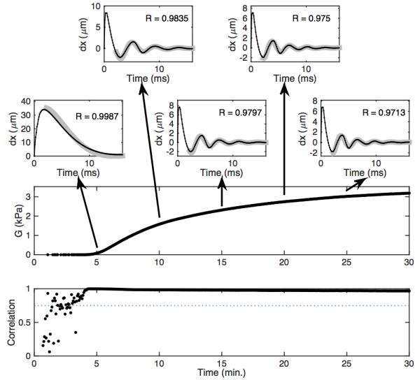
Modulus Estimation via the Free-viscosity Algorithm

Fig. 6 shows representative time-displacement data and associated modulus estimates formed using the free-viscosity algorithm. The top five panels depict experimental time-displacement curves (black) overlying best-fit FDTD models (gray). Examples are shown at five-minute intervals throughout the experiment. The worst-case correlation between FDTD model and experimental data for this experiment was 0.970. The estimated modulus is shown in the next panel. The modulus starts very close to zero and rises to just over 3 kPa. This increase is the result of fibrin mesh formation and the contraction of activated platelets. The next panel shows the estimated shear viscosity. The estimated viscosity peaks around 0.3 Pa s (just after clot formation begins) and falls for the first two minutes of clot formation before it stabilizes around 0.2 Pa s. This shape was not universally observed in our experiments, but is consistent with published viscoelastic data obtained by the ReoRox instrument (32). The noise in the early viscosity estimates occurs because the model considered moduli starting at 10 Pa, so in the early stages of clot formation there is no modeled modulus value that fits the data. The final panel shows the correlation between the best-fit model and the experimental time-displacements. The modulus and viscosity estimates corresponding to correlations below 0.75 were eliminated prior to plotting the data.

Figure 6.

Experimental data analyzed via the free-viscosity algorithm. The top five panels depict experimental time-displacement data (black) overlying best-fit FDTD models (gray). Working downward, the large panels depict estimated modulus, estimated viscosity, and the correlation between the best-fit model and the experimental data. The dotted line in the correlation curve is a threshold value used to reject poor quality estimates.

Fig. 6 shows excellent agreement between the free-viscosity model and the experimental data. It does not however indicate whether this estimator is consistent; that is, do repeated measures of the same blood sample yield the same result. To assess this question we consider variations in modulus measured across four channels within the same cartridge. In an ideal system we would expect these four channels to be identical. However, because of modest variations in mixing, sample temperature, and the speckle pattern underlying the ultrasound signal we expect some variation across channels. To gain qualitative insight into this variation we plot the estimated time-modulus curves for each of four channels across trials using six different blood samples. These results, shown in Fig. 7, show that within each cartridge there is strong agreement between the four channels. Deviations, when they occur, are likely to occur late in coagulation, or even early in thrombolysis.

Figure 7.

Estimated moduli across six different blood samples using the free-viscosity algorithm. Each panel depicts the modulus of each of four channels as a different colored curve. The CV was computed using a one-minute average value centered 20 minutes after the reagents first contacted the blood sample. Variations between samples are to be expected because they were taken from different donors and subjected to different handling.

To quantify SEER consistency we analyzed the modulus 20 minutes into the experiments of Fig. 7. This analysis, shown in Table 4, includes the raw modulus estimates and the associated mean, standard deviation, and CV for the free-viscosity estimator. These results show that the free-viscosity estimator has high precision. We also analyzed the range of modulus estimates in these experiments. The moduli of fresh samples ranged from 2.66 kPa to 3.28 kPa, for a fractional variability of 22%. As a point of comparison, the TEG was shown in (23) to have a range of clot moduli in normal subjects from 0.49 kPa to 1.33 kPa, for a fractional variability of 92%. While the current data set is quite limited, it suggests that the variability of SEER measurements in normal subjects is likely better than that for the TEG. The deviation between modulus estimates for SEER and the TEG reference range is discussed in detail below. The results of table 4 also suggest that overnight refrigeration of samples significantly reduces clot modulus. This result is unsurprising given the well-known negative effects of refrigeration on platelet viability (34).

Table 4.

Estimated shear modulus in Pascals as determined by the free-viscosity estimator. Shear modulus was averaged over a one-minute window centered about twenty minutes from the time of reagent introduction to the blood sample. All coefficients of variation were less than or equal to 2.50%. Samples labeled ‘Fresh’ were drawn into citrated vacutainers and tested in one to four hours. Samples labeled ‘Refrig.’ were also drawn into citrated vacutainers but were refrigerated overnight before testing.

		Exp. 1	Exp. 2	Exp. 3	Exp. 4	Exp. 5	Exp. 6
Subject		A	A	B	C	D	E
Sample		Fresh	Fresh	Fresh	Fresh	Refrig.	Refrig.
Shear Modulus at 20 minutes	Ch. 1	2,642.5	2,658.5	3,366.2	2,653.7	1,582.1	2128.6
	Ch. 2	2,698.2	2,720.7	3,213.9	2,649.2	1,676.4	2,204.6
	Ch. 3	2,656.8	2,734.7	3,280.1	2,769.7	1,654.6	2,093.2
	Ch. 4	2,623.2	2,689.1	3,267.4	2,722.7	1,653.6	2,131.5
Mean Modulus		2,700.7	2,655.2	3,281.9	2,698.8	1,641.7	2,139.5
SD of Modulus		34.0	31.8	63.1	58.0	41.1	46.8
CV of Modulus		1.26%	1.20%	1.92%	2.15%	2.50%	2.19%

Challenges with the Free-viscosity Algorithm

To gain insight into the errors of modulus and viscosity estimates we prepared contour plots showing the correlation coefficient between the model and data as a function of modulus and viscosity. These plots are shown in Fig. 8. In the leftmost panel, corresponding to an estimated modulus of 0.5 kPa, the uncertainty in viscosity covers most of the viscosity values under consideration. As the modulus increases the uncertainty in viscosity shrinks. The correlation map is consistently skewed, that is, an error in estimating viscosity yields an error in estimating modulus.

Figure 8.

Contour plots depicting the normalized correlation between the free-viscosity model and experimental data for measured shear moduli of 0.5, 1.75, and 3.0 kPa.

Modulus Estimation via the Fixed-viscosity Algorithm

To overcome the free-viscosity estimator’s coupling of viscosity and modulus errors, we implemented a fixed-viscosity estimator. This algorithm estimates modulus while holding viscosity constant. The fixed-viscosity algorithm will exhibit a lower correlation with the data as it has fewer degrees of freedom. Furthermore, it will bias modulus estimates in cases where the viscosity deviates from the assumed value. In many cases however, these limitations may be outweighed by the lower variance of the modulus estimates from the fixed-viscosity algorithm.

Fig. 9 shows time-displacement data and associated modulus estimates formed using the fixed-viscosity algorithm applied to the same data as that presented in Fig. 6. The worst-case correlation between FDTD model and experimental data for this experiment was 0.968. As expected, the fixed-viscosity model shows lower correlations with the data than the free-viscosity model. During the liquid blood phase (prior to clotting) the fixed-viscosity model shows a higher correlation than the free-viscosity model. This is because the fixed-viscosity models were formed at moduli as low as 0.001 Pa, while the free-viscosity models only considered moduli down to 10 Pa.

Figure 9.

Experimental data analyzed via the fixed-viscosity algorithm. The top five panels depict experimental time-displacement data in black overlying best-fit FDTD models in gray. Working downward, the large panels depict estimated modulus and the correlation between the best-fit model and the experimental data. The dotted line in the correlation curve is a 0.75 threshold value used to reject poor quality estimates.

We assessed consistency for the fixed-viscosity algorithm by plotting the estimated moduli across all six experiments, as shown in Fig. 10. Results show a slight improvement of consistency over the free-viscosity algorithm. This is expected as the correlation maps of Fig. 8 show that the viscosity estimates are error prone and that errors in estimating viscosity introduce errors in the modulus estimate. The higher error of the free-viscosity algorithm is also consistent with the performance bound derived below.

Figure 10.

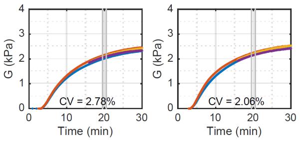
Estimated moduli across six different blood samples using the fixed-viscosity algorithm. Each panel depicts the modulus of each of four channels as a different colored curve. The CV was computed using a one minute average value centered 20 minutes after the reagents first contacted the blood sample. Samples labeled ‘Fresh’ were drawn into citrated vacutainers and tested within four hours. Samples labeled ‘Refrig.’ were also drawn into citrated vacutainers but were refrigerated overnight before warming and testing.

Table 5 shows the raw modulus estimates and the associated mean, standard deviation, and CV for the fixed-viscosity estimator. These results show that the fixed-viscosity estimator has high precision. In fact, the precision of the fixed-viscosity estimator is slightly better than that of the free-viscosity estimator.

Table 5.

Estimated shear modulus in Pascals as determined by the fixed-viscosity estimator with the viscosity fixed at 0.25 Pa s. Shear modulus values were found by estimates over a one minute window centered about twenty minutes from the time of reagent introduction to the blood sample. All coefficients of variation were less than or equal to 1.84%.

		Exp. 1	Exp. 2	Exp. 3	Exp. 4	Exp. 5	Exp. 6
Subject		A	A	B	C	D	E
Sample		Fresh	Fresh	Fresh	Fresh	Refrig.	Refrig.
Shear Modulus at 20 minutes	Ch. 1	2,656.2	2,655.0	3,373.1	2,660.1	1,592.1	2,144.7
	Ch. 2	2,728.3	2,717.3	3,233.5	2,667.8	1,637.5	2,207.3
	Ch. 3	2,754.4	2,676.4	3,309.9	2,727.2	1,653.9	2,112.1
	Ch. 4	2,711.5	2,637.0	3,270.5	2,743.0	1,636.9	2,148.4
Mean Modulus		2,712.6	2,671.4	3,296.7	2,699.5	1,630.1	2,153.1
SD of Modulus		41.5	34.6	59.7	41.7	26.5	39.7
CV of Modulus		1.53%	1.29%	1.81%	1.54%	1.63%	1.84%

Assessing the validity of SEER

The results presented here indicate that SEER, in either variant, is a precise and consistent method of estimating modulus. Although we are aware of no appropriate gold standard to which to compare SEER, the excellent agreement between the analytical model and the FDTD cylindrical model provides a strong indication that the algorithm is accurate.

We further validate SEER by comparing the modulus estimated using the fixed-viscosity algorithm to a simple calculation based on resonant frequency. The period of resonance at 25 minutes in Fig. 8 is approximately 3 ms, which corresponds to a resonant frequency of 333 Hz. Substituting this frequency into Eq. B-12 and assuming a density of 1060 kg/m³ yields a predicted modulus of 3.54 kPa. The fixed-viscosity algorithm estimated the modulus as 3.0 kPa. This 18% discrepancy is not surprising given the differences in geometry between the two approaches. Nonetheless, this reasonable level of agreement supports the validity of FDTD model based estimation.

An important question for any test is whether the act of testing alters the process being tested. While SEER applies relatively small forces, at a very low duty cycle, there is the concern that the applied radiation force disrupts the clot as it forms. If this mechanism of interference existed, one would expect that samples measured continuously by SEER would exhibit a lower modulus than samples measured intermittently. We assessed the impact of SEER on clot formation using modified software in which channels 1 and 2 followed a standard acquisition sequence while channels 3 and 4 were left dormant until 15 minutes had passed after the first acquisition on channels 1 and 2. ‘Fresh’ citrated blood samples were tested using kaolin activation. The modulus estimates from two trials were computed using the fixed-viscosity algorithm and are shown in figure 11. While the variance between channels is somewhat higher than that seen in our prior experiments, there is no sign of significantly increased modulus in channels 3 and 4.

Figure 11.

Estimated moduli from two blood samples using the fixed-viscosity algorithm with a modified acquisition sequence to assess the impact of acoustic radiation force on clot formation. Channels 3 and 4 were dormant until 15 minutes after mixing. These results show that ultrasound radiation force has no significant impact on clot formation.

Fundamental Limits on SEER Performance

To gain deeper insight into the performance of the free-viscosity and fixed-viscosity algorithms we estimated the Cramér-Rao Lower Bound (CRLB) as derived in Appendix C. We used the FDTD models for the mean signals required by the bound. Across all combinations of modulus and viscosity we scaled the peak-to-peak displacement to be 5 microns; a grossly pessimistic assumption for low moduli. We also assumed that the standard deviation of displacement estimates was 84.2 nm, as predicted by equation (4). The results of this analysis, presented in table 6, predict SEER precision better than 0.5% for modulus estimates and 3% for viscosity estimates. We note that there is little predicted difference between the performance of the fixed-viscosity and free-viscosity algorithms, which is consistent with our experimental observations. Predicted errors are roughly an order of magnitude smaller than those observed experimentally. This is not surprising given the potential variability introduced by imperfect mixing, inconsistent heating, and imperfect modeling of the ultrasound beam and chamber geometry. Nonetheless, we are encouraged to see that this analysis suggests significant opportunity to improve the performance of our system. The CRLB prediction incorporates many assumptions about system performance. We can improve theoretical performance further by increasing the PRF, increasing the induced displacements, reducing displacement estimation errors, processing early displacement estimates which are currently discarded, and adjusting the chamber geometry.

Table 6.

Lower bounds on SEER performance as predicted by the expressions of Appendix C for the system configuration of this paper. Peak to peak displacement was assumed to be 5 microns and the standard deviation of displacement estimates was assumed to be 84.2 nm.

Modulus (kPa)	Viscosity (Pa s)	Free-Viscosity SEER		Fixed-Viscosity SEER
		σμ (kPa)	ση (Pa s)	σμ (kPa)	ση (Pa s)
0.5 kPa	0.25 Pa s	2.2 (0.4%)	0.0034 (1.3%)	1.8 (0.4%)	N/A
1.75 kPa	0.25 Pa s	4.2 (0.2%)	0.0053 (2.1%)	4.0 (0.2%)	N/A
3.0 kPa	0.25 Pa s	7.6 (0.3%)	0.0069 (2.8%)	7.1 (0.2%)	N/A

Comparison with Literature Estimates of Clot Modulus

The four fresh blood experiments presented in tables 4 and 5 exhibited a range of shear moduli from 2.7 to 3.3 kPa. The best-known technique for viscoelastic clot measurement, the Thromboelastogram (TEG), has a normal range of MA from 49.7 to 72.7 mm for kaolin induced human blood clots. This MA range corresponds to shear moduli from 0.49 to 1.33 kPa for normal volunteers (23). Likewise, the normal range for the ROTEM is 49-71 mm (0.48 to 1.22 kPa) for kaolin induced human blood clots from healthy subjects (24). The ReoRox package insert describes a normal modulus range for thromboplastin induced clots in citrated samples extending from 0.77 kPa to 2.18 kPa. Huang et al (14) utilized a shear wave approach to measure shear moduli ranging from approximately 0.20 to 0.64 kPa in whole porcine blood. Bernal et al (25) also used shear wave velocity to estimate shear modulus of up to 1.3 kPa in whole porcine blood.

In all comparisons with the literature we find that SEER yields higher modulus estimates. We believe that the discrepancies between SEER and the literature estimates can be explained by differences in methodology. A significant difference between SEER and prior methods is in the time course of force application. SEER applies a forcing pulse for less than 15 μs, while the TEG, for example, applies an oscillating force with a period of 10 s. This difference in forcing functions means that SEER is interrogating the clot with a forcing frequency over five orders of magnitude higher than the TEG. Given the viscoelastic nature of the clot it should come as no surprise that these instruments yield different modulus estimates. The literature methods also apply significant shear stress to the blood during clot formation. We hypothesize that this shear stress disrupts clot formation, much as stirring gelatin during its formation will yield a softer gel. We believe that this shearing applies a downward bias to TEG and ROTEM estimates in particular when compared to SEER. We note that the normal range for ReoRox measurements roughly 60% greater than that for TEG and ROTEM. This difference may be due to different shear rates and excitation frequencies applied by these technologies. The porcine blood studies (14,25) differed from the current study in a number of ways that would reduce their clot stiffness. These studies initiated clotting using only added calcium, rather than the kaolin we use. Kaolin causes more aggressive activation of the intrinsic pathway and in turn activates platelets to form a significantly stiffer clot. Bernal et al observed that the clots in their study contracted, releasing some of their intrinsic tension and reducing the clot’s structural stiffness. Thus we expect the porcine blood clots to be lower in modulus relative to our clots, consistent with observation.

Future Work

In future work we intend to further validate SEER by comparing directly to measurements from a conventional rheometer. Doing so with blood is difficult because the dynamics of clot formation are temperature and shear stress dependent. Given that no rheometer will exactly mimic our test cartridge, we believe it will be more meaningful to test a clot mimicking material. Such a material must have viscoelastic and ultrasound properties that reasonably mimic those of a formed clot. We are actively working to develop such a material, but doing so is beyond the scope of the current paper.

As good as our current SEER implementation is, we see a number of ways to further improve performance. We observe that the initial positive displacement peak is generally poorly modeled. We have avoided this issue in the current study by masking the first 18 displacement estimates prior to fitting. We expect to improve modeling of this portion of the time-displacement curve by developing a rigorous force model based on experimental measurements of the forcing ultrasound beam. We intend to further improve accuracy by more accurately modelling the geometry of the test chamber. We intend optimize electrical impedance matching to increase radiation force induced displacement.

Clinical Significance

SEER precision on the order of 2% compares favorably to the TEG, with its precision of 6% in measurements of maximum clot stiffness (10). Given that the TEG has shown broad utility in a range of clinical settings, SEER’s improved precision and ease of use should open new clinical applications where speed to result and higher precision are essential. SEER technology is currently being tested in cardiac surgery, where faster results are expected to enable rigorous testing in circumstances where time pressure has traditionally led to widespread use of “shotgun therapy.” Ongoing tests in complex spinal surgery will assess whether SEER’s faster results replace “shotgun therapy” in that application. Testing in cancer patients will explore whether the improved precision of SEER enables early detection of coagulopathies associated with malignancy and chemotherapy. In these and other clinical applications, SEER has the potential to provide rigorous data to inform the treatment of complex bleeding. Such information should improve patient outcomes while reducing healthcare costs.

Conclusion

This paper has described SEER Sonorheometry, a novel method of estimating the shear modulus of soft biomaterials in vitro. Two variants of SEER were presented in which the viscosity of the sample was either estimated or assumed to have a specific value. The fixed-viscosity algorithm exhibited slightly lower variance, but likely incorporates some bias when the viscosity differs from the assumed value. SEER shows significant potential as a tool for measuring the evolving mechanics of coagulation in vitro. This technology has the potential to deliver comprehensive and time critical information needed to improve patient outcomes in surgery and clinical care.

Appendix A: Finite Difference Formulation

Our formulation of the Finite Difference Time Domain model is built upon a velocity – stress formulation of the shear wave equation (22,26). We expand upon traditional formulations by including a term to account for viscous loss.

$$\rho \frac{\partial }{\partial t}\overrightarrow{v}\phantom{)}(\overrightarrow{x},t)\phantom{(}=\nabla \cdot \sigma \phantom{)}(\overrightarrow{x},t)\phantom{(}+\overrightarrow{F}\phantom{)}(\overrightarrow{x},t)\phantom{(}$$ (A-1)

$$\frac{\partial }{\partial t}\sigma \phantom{)}(\overrightarrow{x},t)\phantom{(}=\left(\mu +\eta \frac{\partial }{\partial t}\right)\left[\left(\nabla \overrightarrow{v}(\overrightarrow{x},t)\right)+{\left(\nabla \overrightarrow{v}(\overrightarrow{x},t)\right)}^T\right]$$ (A-2)

Our analysis assumes an axisymmetric test chamber, which suggests the use of cylindrical coordinates. Representing Eq. A-1 in cylindrical coordinates and expanding the vector velocity into its constituent components yields:

$$\frac{\partial {\sigma }_{\mathit{rr}}}{\partial r}+\frac{1}{r}\frac{\partial {\sigma }_{r\varphi }}{\partial \varphi }+\frac{\partial {\sigma }_{\mathit{rz}}}{\partial z}+\frac{1}{r}\left({\sigma }_{\mathit{rr}}-{\sigma }_{\varphi \varphi }\right)+F_r=\rho \frac{\partial v_r}{\partial t}$$ (A-3a)

$$\frac{\partial {\sigma }_{r\varphi }}{\partial r}+\frac{1}{r}\frac{\partial {\sigma }_{\varphi \varphi }}{\partial \varphi }+\frac{\partial {\sigma }_{\varphi z}}{\partial z}+\frac{2}{r}{\sigma }_{r\varphi }+F_{\varphi }=\rho \frac{\partial v_{\varphi }}{\partial t}$$ (A-3b)

$$\frac{\partial {\sigma }_{\mathit{rz}}}{\partial r}+\frac{1}{r}\frac{\partial {\sigma }_{\varphi z}}{\partial \varphi }+\frac{\partial {\sigma }_{\mathit{zz}}}{\partial z}+\frac{1}{r}{\sigma }_{\mathit{rz}}+F_z=\rho \frac{\partial v_z}{\partial t}$$ (A-3c)

We further simplify by recognizing that the only body force, the applied ultrasound radiation force, acts only in the z direction. We set F_ϕ = F_r = 0. Since our test chamber and the applied radiation force are entirely axisymmetric, we set all dependencies upon ϕ equal to zero. Applying these simplifications to Eqs. A-3 yields:

$$\frac{\partial {\sigma }_{\mathit{rz}}}{\partial z}=\rho \frac{{\partial }^2{u}_r}{\partial t^2}$$ (A-4a)

$$0=0$$ (A-4b)

$$\frac{\partial {\sigma }_{\mathit{rz}}}{\partial r}+\frac{1}{r}{\sigma }_{\mathit{rz}}+F_z=\rho \frac{{\partial }^2{u}_z}{\partial t^2}$$ (A-4c)

We follow a similar strategy to expand Eq. A-2, to yield:

$$\frac{\partial {\sigma }_{\mathit{rz}}}{\partial t}=\left(\mu +\eta \frac{\partial }{\partial t}\right)\left(\frac{\partial v_r}{\partial z}+\frac{\partial v_z}{\partial r}\right)$$ (A-5)

Collecting Eqs. A-4 and Eq. A-5 yields:

$$\rho \frac{\partial v_r}{\partial t}=\frac{\partial {\sigma }_{\mathit{rz}}}{\partial z}$$ (A-6a)

$$\rho \frac{\partial v_z}{\partial t}=\frac{\partial {\sigma }_{\mathit{rz}}}{\partial r}+\frac{1}{r}{\sigma }_{\mathit{rz}}+F_z$$ (A-6b)

$$\frac{\partial {\sigma }_{\mathit{rz}}}{\partial t}=\left(\mu +\eta \frac{\partial }{\partial t}\right)\left(\rho \frac{\partial v_r}{\partial t}+\rho \frac{\partial v_z}{\partial t}\right)$$ (A-6c)

Eqs. A-6a through A-6c form a system of partial differential equations that predict how radiation force will induce shear waves and how those induced shear waves will interact. This system of equations is amenable to a finite difference solution using a staggered grid approach, similar to the Yee method (27). The finite difference representation of Eqs. A-6a through A-6c are:

$${v_r}_{j,k}^{i+1}={v_r}_{j,k}^i+\frac{\Delta t}{\rho \Delta z}\left({{\sigma }_{\mathit{rz}}}_{j,k+\frac{1}{2}}^i-{{\sigma }_{\mathit{rz}}}_{j,k-\frac{1}{2}}^i\right)$$ (A-7a)

$${v_z}_{j+\frac{1}{2},k+\frac{1}{2}}^{i+1}={v_z}_{j+\frac{1}{2},k+\frac{1}{2}}^i+\frac{\Delta t}{\rho }\left(\frac{1}{\Delta r}\left({{\sigma }_{\mathit{rz}}}_{j+1,k+\frac{1}{2}}^i-{{\sigma }_{\mathit{rz}}}_{j,k+\frac{1}{2}}^i\right)+\frac{1}{2(j+\frac{1}{2})\Delta r}\left({{\sigma }_{\mathit{rz}}}_{j,k+\frac{1}{2}}^i-{{\sigma }_{\mathit{rz}}}_{j+1,k+\frac{1}{2}}^i\right)+{F_z}_{j++\frac{1}{2},k+\frac{1}{2}}^i\right)$$ (A-7b)

$${{\sigma }_{\mathit{rz}}}_{j,k+\frac{1}{2}}^{i+1}={{\sigma }_{\mathit{rz}}}_{j,k+\frac{1}{2}}^i+\frac{\mu \Delta t}{\Delta z}\left({v_r}_{j,k+1}^i-{v_r}_{j,k}^i\right)+\frac{\mu \Delta t}{\Delta z}\left({v_r}_{j+\frac{1}{2},k++\frac{1}{2}}^i-{v_r}_{j-\frac{1}{2},k+\frac{1}{2}}^i\right)+\frac{\eta }{\Delta z}\left({v_r}_{j,k+1}^{i+1}-{v_r}_{j,k+1}^i-{v_r}_{j,k}^{i+1}+{v_r}_{j,k}^i\right)+\frac{\eta }{\Delta z}\left({v_z}_{j+\frac{1}{2},k+\frac{1}{2}}^{i+1}-{v_z}_{j+\frac{1}{2},k+\frac{1}{2}}^i-{v_z}_{j-\frac{1}{2},k+\frac{1}{2}}^{i+1}+{v_z}_{j-\frac{1}{2},k+\frac{1}{2}}^i\right)$$ (A-7c)

This formulation was implemented in MATLAB (Natick, MA) using the staggered grid approach shown in Fig. A-1 with a default sampling interval of 100 μm. Each computational cycle consisted of two steps. In the first, the velocity components were computed via Eqs. A-7a and A-7b. In the next step shear was computed using Eq. A-7c. Time-dependent velocities were integrated numerically using cumulative trapezoidal integration (cumtrapz in MATLAB) to determine the time-varying displacement.

Figure A-1.

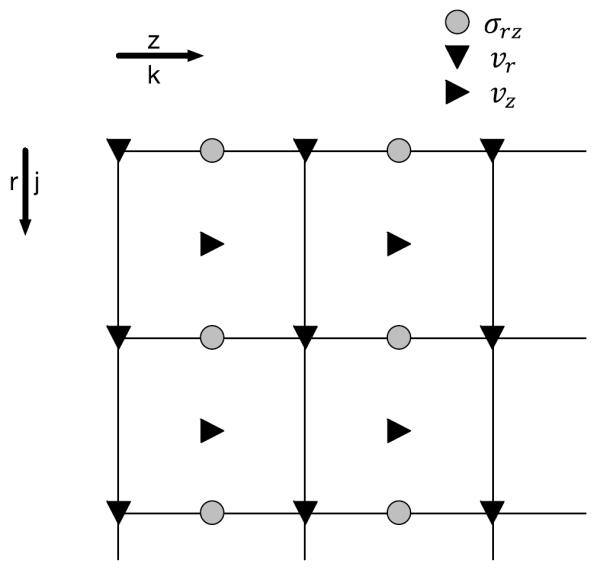
FDTD model staggered grid geometry.

Appendix B: Analytical Model

This analysis is based upon the Cauchy-Navier Equation for linear elasticity. We utilize a formulation incorporating viscoelastic material properties.

$$\left(\left(\lambda +\mu +({\eta }_{\mathit{p}}+{\eta }_{\mathit{s}})\frac{\mathit{d}}{\mathit{dt}}\cdot \right)\nabla (\nabla \cdot \overrightarrow{\mathit{u}}(\overrightarrow{\mathit{x}},\mathit{t}\left)\right)\right)+\left(\left(\mu +{\eta }_{\mathit{s}}\frac{\mathit{d}}{\mathit{dt}}\cdot \right){\nabla }^2\overrightarrow{\mathit{u}}(\overrightarrow{\mathit{x}},\mathit{t})\right)-\rho \frac{{\mathit{d}}^2}{{\mathit{dt}}^2}\overrightarrow{\mathit{u}}(\overrightarrow{\mathit{x}},\mathit{t})=\overrightarrow{\mathit{F}}(\overrightarrow{\mathit{x}},\mathit{t})$$ (B-1)

To simplify analysis we assume an infinitely long cylindrical test chamber with radiation force applied to the central axis. We apply these simplifications to the components of Eq. B-1:

$$\nabla \phantom{)}(\nabla \cdot \overrightarrow{\mathit{u}}\phantom{)}(\overrightarrow{\mathit{x}},\mathit{t})\phantom{(})\phantom{(}=\nabla \left(\frac{1}{\mathit{r}}\frac{\mathit{d}}{\mathit{dr}}\phantom{)}({\mathit{ru}}_{\mathit{r}})\phantom{(}+\frac{1}{\mathit{r}}\frac{\mathit{d}}{\mathit{d}\varphi }{\mathit{u}}_{\varphi }+\frac{\mathit{d}}{\mathit{dz}}{\mathit{u}}_{\mathit{z}}\right)$$ (B-2a)

$${\nabla }^2\overrightarrow{\mathit{u}}\phantom{)}(\overrightarrow{\mathit{x}},\mathit{t})\phantom{(}=\left[{\nabla }^2{\mathit{u}}_{\mathit{r}}-\frac{1}{{\mathit{r}}^2}{\mathit{u}}_{\mathit{r}}-\frac{2}{{\mathit{r}}^2}\frac{\mathit{d}}{\mathit{d}\varphi }{\mathit{u}}_{\varphi }\right]\widehat{\mathit{r}}+\left[{\nabla }^2{\mathit{u}}_{\varphi }-\frac{1}{{\varphi }^2}{\mathit{u}}_{\varphi }-\frac{2}{{\mathit{r}}^2}\frac{\mathit{d}}{\mathit{d}\varphi }{\mathit{u}}_{\mathit{r}}\right]\widehat{\varphi }+\phantom{]}[{\nabla }^2{\mathit{u}}_{\mathit{z}}]\phantom{[}\widehat{\mathit{z}}$$ (B-2b)

Because of cylindrical symmetry and the assumed infinite length of the chamber we can set all derivatives with respect to ϕ and z equal to zero.

$$\nabla \phantom{)}(\nabla \cdot \overrightarrow{\mathit{u}}\phantom{)}(\overrightarrow{\mathit{x}},\mathit{t})\phantom{(})\phantom{(}=\nabla \left(\frac{1}{\mathit{r}}\frac{\mathit{d}}{\mathit{dr}}\left({\mathit{ru}}_{\mathit{r}}\right)\right)\widehat{\mathit{r}}$$ (B-3a)

$${\nabla }^2\overrightarrow{\mathit{u}}\phantom{)}(\overrightarrow{\mathit{x}},\mathit{t})\phantom{(}=\left[{\nabla }^2{\mathit{u}}_{\mathit{r}}-\frac{1}{{\mathit{r}}^2}{\mathit{u}}_{\mathit{r}}\right]\widehat{\mathit{r}}+0\widehat{\varphi }+\phantom{]}[{\nabla }^2{\mathit{u}}_{\mathit{z}}]\phantom{[}\widehat{\mathit{z}}$$ (B-3b)

Expanding gradients and Laplacians as appropriate, and setting derivatives with respect to ϕ and z equal to zero yields:

$$\nabla \phantom{)}(\nabla \cdot \overrightarrow{\mathit{u}}\phantom{)}(\overrightarrow{\mathit{x}},\mathit{t})\phantom{(})\phantom{(}=\left[\frac{\mathit{d}}{\mathit{dr}}\left(\frac{1}{\mathit{r}}\frac{\mathit{d}}{\mathit{dr}}\phantom{)}({\mathit{ru}}_{\mathit{r}})\phantom{(}\right)\right]\widehat{\mathit{r}}+0\widehat{\varphi }+0\widehat{\mathit{z}}$$ (B-4a)

$${\nabla }^2\overrightarrow{\mathit{u}}\phantom{)}(\overrightarrow{\mathit{x}},\mathit{t})\phantom{(}=\left[\frac{1}{\mathit{r}}\frac{\mathit{d}}{\mathit{dr}}\left(\mathbf{r}\frac{\mathit{r}}{\mathit{dr}}{\mathit{u}}_{\mathit{r}}\right)+\frac{1}{{\mathit{r}}^2}{\mathit{u}}_{\mathit{r}}\right]\widehat{\mathit{r}}+0\widehat{\varphi }+\left[\frac{1}{\mathit{r}}\frac{\mathit{d}}{\mathit{dr}}\left(\mathbf{r}\frac{\mathit{d}}{\mathit{dr}}{\mathit{u}}_{\mathit{z}}\right)\right]\widehat{\mathit{z}}$$ (B-4b)

This result shows that there are no cross terms between the radial and axial displacements. Our system measures axial displacement, so we discard the radial displacement term after substituting Eqs. B-4a and B-4b into Eq. B-1, and assuming that the force is applied impulsively at time zero and is a spatial impulse at the center of the measurement cylinder.

$$\left(\left(\mu +{\eta }_{\mathit{s}}\frac{\mathit{d}}{\mathit{dt}}\cdot \right)\left(\frac{{\mathit{d}}^2}{{\mathit{dr}}^2}{\mathit{u}}_{\mathit{z}}\phantom{)}(\mathit{r},\mathit{t})\phantom{(}+\frac{1}{\mathit{r}}\frac{\mathit{d}}{\mathit{dr}}{\mathit{u}}_{\mathit{z}}\phantom{)}(\mathit{r},\mathit{t})\phantom{(}\right)\right)-\rho \frac{{\mathit{d}}^2}{{\mathit{dt}}^2}{\mathit{u}}_{\mathit{z}}\phantom{)}(\mathit{r},\mathit{t})\phantom{(}=\delta \phantom{)}(\mathit{t})\phantom{(}\delta \phantom{)}(\mathit{r})\phantom{(}∕\mathit{r}$$ (B-5)

We now utilize the Hankel Transform as defined in Eq. B-6 (28) to solve this partial differential equation.

$$\tilde{\mathit{u}}\phantom{)}({\xi }_{\mathit{i}},\mathit{t})\phantom{(}={\int }_0^{{\mathit{R}}_{\mathit{c}}}\mathit{ru}\phantom{)}(\mathit{r},\mathit{t})\phantom{(}{\mathit{J}}_0\phantom{)}({\xi }_{\mathit{i}}\mathit{r})\phantom{(}\mathit{dr}$$ (B-6)

where R_c is the radius of the cylinder, J₀(x) is 0^th order Bessel function of the first kind, and ξ_i = λ_i/R_c where λ_i is the i^th root of the 0^th order Bessel function of the first kind. Performing the Hankel Transform on Eq. B-5 yields:

$$-\mu {{\xi }_{\mathit{i}}}^2\tilde{\mathit{u}}\phantom{)}({\xi }_{\mathit{i}},\mathit{t})\phantom{(}-{\eta }_{\mathit{s}}{{\xi }_{\mathit{i}}}^2\frac{\mathit{d}}{\mathit{dt}}\tilde{\mathit{u}}\phantom{)}({\xi }_{\mathit{i}},\mathit{t})\phantom{(}-\rho \frac{{\mathit{d}}^2}{{\mathit{dt}}^2}\tilde{\mathit{u}}\phantom{)}({\xi }_{\mathit{i}},\mathit{t})\phantom{(}=\delta \phantom{)}(\mathit{t})\phantom{(}$$ (B-7)

The application of the Hankel Transform has reduced a partial differential equation to an ordinary differential equation. Assuming that $\tilde{\mathit{u}}({\xi }_{\mathit{i}},0)=0$ and that $\frac{\mathit{d}}{\mathit{dt}}\tilde{\mathit{u}}({\xi }_{\mathit{i}},\mathit{t})=0$ then:

$$\tilde{\mathit{u}}\phantom{)}({\xi }_{\mathit{i}},\mathit{t})\phantom{(}=\frac{1}{\sqrt{\mathit{A}}}{\mathit{e}}^{-{t\eta }_{\mathit{s}}{{\xi }_{\mathit{i}}}^2∕2\rho }\left({\mathit{e}}^{-\mathit{t}\sqrt{\mathit{A}}∕2\rho }-{\mathit{e}}^{\mathit{t}\sqrt{\mathit{A}}∕2\rho }\right)$$ (B-8)

where A = ξ_i²(η_s²ξi² − 4μρ). The finite Hankel Transform can be inverted using Eq. B-9 [equation 45 on page 83 of (28)].

$$\mathit{f}\phantom{)}(\mathit{x})\phantom{(}=\frac{2}{{{\mathit{R}}_{\mathit{c}}}^2}\sum _{\mathit{i}=1}^{\infty }\tilde{\mathit{f}}\phantom{)}({\xi }_{\mathit{i}})\phantom{(}\frac{{\mathit{J}}_0\left({\xi }_{\mathit{i}}\mathit{x}\right)}{{\left[{\mathit{J}}_1\right({\xi }_{\mathit{i}}{\mathit{R}}_{\mathit{c}}\left)\right]}^2}$$ (B-9)

Applying the inversion formula of Eq. B-9 to Eq. B-8 yields an expression for the time-dependent displacement.

$$\mathbf{u}\phantom{)}(\mathit{r},\mathit{t})\phantom{(}=\frac{2}{{{\mathit{R}}_{\mathit{c}}}^2}\sum _{\mathit{i}=1}^{\infty }\frac{{\mathit{J}}_0\left({\xi }_{\mathit{i}}\mathit{r}\right)}{\sqrt{\mathit{A}}{\left[{\mathit{J}}_1\right({\xi }_{\mathit{i}}{\mathit{R}}_{\mathit{c}}\left)\right]}^2}{\mathit{e}}^{-{t\eta }_{\mathit{s}}{{\xi }_{\mathit{i}}}^2∕2\rho }\left({\mathit{e}}^{-\mathit{t}\sqrt{\mathit{A}}∕2\rho }-{\mathit{e}}^{\mathit{t}\sqrt{\mathit{A}}∕2\rho }\right)$$ (B-10)

In comparing Eq. B-10 to results from a simplified FDTD model we see that analytical model consistently exhibits high frequency content that is not visible in the FDTD model. We believe that this discrepancy is a result of the finite spatial sampling interval of the FDTD model. We have found empirically that the analytical model is in good agreement with the FDTD model when we include only terms up to those for which there is at least 1.5 samples per half cycle of the Bessel function. This truncated model, shown as Eq. B-10 shows excellent agreement with the simplified FDTD model.

$$\widehat{\mathbf{u}}(\mathit{r},\mathit{t})=\frac{2}{{{\mathit{R}}_{\mathit{c}}}^2}\sum _{\mathit{i}=1}^{2{\mathit{R}}_{\mathit{c}}∕3\Delta \mathit{x}}\frac{{\mathit{J}}_0\left({\xi }_{\mathit{i}}\mathit{r}\right)}{\sqrt{\mathit{A}}{\left[{\mathit{J}}_1\right({\xi }_{\mathit{i}}{\mathit{R}}_{\mathit{c}}\left)\right]}^2}{\mathit{e}}^{-{t\eta }_{\mathit{s}}{{\xi }_{\mathit{i}}}^2∕2\rho }\left({\mathit{e}}^{-\mathit{t}\sqrt{\mathit{A}}∕2\rho }-{\mathit{e}}^{\mathit{t}\sqrt{\mathit{A}}∕2\rho }\right)$$ (B-10)

where Δx is the spatial sampling interval of the FDTD model. The terms of the sum take on two different forms depending upon whether A > 0, in which case the system is overdamped, or A < 0, in which case the system is underdamped. In the underdamped case the first term of the series is a sine wave under a decaying exponential envelope. Assuming that the system has very low damping, the resonant frequency is:

$${\mathit{f}}_0={}^{\sqrt{\mathit{A}}}/_{2\pi 2\rho }={}^{-\mathit{i}\sqrt{{{\xi }_1}^2({{\eta }_{\mathit{s}}}^2{{\xi }_1}^2-4\mu \rho )}}/_{4\pi \rho }\approx {}^{-\mathit{i}\sqrt{{{\xi }_1}^2(-4\mu \rho )}}/_{4\pi \rho }=\frac{{\xi }_1}{2\pi }\sqrt{\frac{\mu }{\rho }}=\frac{2.4048}{2\pi {\mathit{R}}_{\mathit{c}}}\sqrt{\frac{\mu }{\rho }}$$ (B-11)

where the factor of 2π is required to convert from radial to temporal frequency. The shear modulus can be estimated from the resonant frequency:

$$\mu =\rho {\left(\frac{2\pi {\mathit{f}}_0{\mathit{R}}_{\mathit{c}}}{2.4048}\right)}^2$$ (B-12)

The concept of resonant frequency is only meaningful when the resonant chamber is under-damped. The system is under-damped when A < 0, or equivalently when:

$$\mu >\frac{{{\eta }_{\mathit{s}}}^2{{\xi }_{\mathit{i}}}^2}{4\rho }$$ (B-13)

For our geometry assuming a blood density of 1060 kg/m³ and a shear viscosity of approximately 0.25 Pa s, the system will be under-damped for moduli greater than 19.3 Pa.

Appendix C: Cramér-Rao Lower Bound on SEER

We begin our analysis from the formulation derived by Scharf in (33). The lower bound on the variance C_ii of estimates of the parameter θ_i is:

$${\mathit{C}}_{\mathit{ii}}\ge {\left({\mathit{J}}^{-1}\right)}_{\mathit{ii}}$$ (C-1)

where J is the Fisher information matrix. The elements of the Fisher information matrix, for a single realization of data, are defined by equation 6.134 of (33):

$${\mathit{J}}_{\mathit{ij}}=\frac{1}{2}\mathit{tr}\left[{\mathit{R}}^{-1}\frac{\partial \mathit{R}}{{\partial \theta }_{\mathit{i}}}{\mathit{R}}^{-1}\frac{\partial \mathit{R}}{{\partial \theta }_{\mathit{j}}}\right]+\frac{{\partial m}^{\mathit{t}}}{{\partial \theta }_{\mathit{i}}}{\mathit{R}}^{-1}\frac{\partial m}{{\partial \theta }_{\mathit{j}}}$$ (C-2)

where tr[X] is the trace of matrix X, R is the expected covariance matrix of the observed data, and m is the expected mean of the observed data. In SEER the observed data is the vector of time-displacement estimates. We assume that the noise in the displacement estimates is generally uncorrelated so that the covariance matrix can be modeled as an identity matrix scaled by the variance of the displacement estimates.

$$\mathit{R}=\frac{1}{{\sigma }_{\mathit{x}}^2}\mathit{I}$$ (C-3)

where ${\sigma }_{\mathit{x}}^2$ is the variance of the displacement estimates. Assuming that the error covariance does not depend upon the parameter (either θ_i or θ_j) and that the covariance can be represented as in (C-3), then (C-2) can be simplified as:

$${\mathit{J}}_{\mathit{ij}}=\frac{\partial {\mathit{m}}^{\mathit{t}}}{{\partial \theta }_{\mathit{i}}}{\mathit{R}}^{-1}\frac{\partial \mathit{m}}{{\partial \theta }_{\mathit{j}}}=\frac{\partial {\mathit{m}}^{\mathit{t}}}{{\partial \theta }_{\mathit{i}}}{\left[\frac{1}{{\sigma }_{\mathit{x}}^2}\mathit{I}\right]}^{-1}\frac{\partial \mathit{m}}{{\partial \theta }_{\mathit{j}}}=\frac{1}{{\sigma }_{\mathit{x}}^2}\frac{\partial {\mathit{m}}^{\mathit{t}}}{{\partial \theta }_{\mathit{i}}}\frac{\partial \mathit{m}}{{\partial \theta }_{\mathit{j}}}$$ (C-4)

For the free-viscosity estimator we estimate both the viscosity and the modulus, so the Fisher Information Matrix is:

$$\mathit{J}=\left[\begin{array}{cc}\hfill \frac{1}{{\sigma }_{\mathit{x}}^2}\frac{\partial {\mathit{m}}^{\mathit{t}}}{{\partial \theta }_{\mu }}\frac{\partial m}{{\partial \theta }_{\mu }}\hfill & \hfill \frac{1}{{\sigma }_{\mathit{x}}^2}\frac{\partial {\mathit{m}}^{\mathit{t}}}{{\partial \theta }_{\mu }}\frac{\partial m}{{\partial \theta }_{\eta }}\hfill \\ \hfill \hfill & \hfill \hfill \\ \hfill \frac{1}{{\sigma }_{\mathit{x}}^2}\frac{\partial {\mathit{m}}^{\mathit{t}}}{{\partial \theta }_{\eta }}\frac{\partial m}{{\partial \theta }_{\mu }}\hfill & \hfill \frac{1}{{\sigma }_{\mathit{x}}^2}\frac{\partial {\mathit{m}}^{\mathit{t}}}{{\partial \theta }_{\eta }}\frac{\partial m}{{\partial \theta }_{\eta }}\hfill \end{array}\right]=\frac{1}{{\sigma }_{\mathit{x}}^2}\left[\begin{array}{cc}\hfill \frac{{\partial m}^{\mathit{t}}}{{\partial \theta }_{\mu }}\frac{\partial m}{{\partial \theta }_{\mu }}\hfill & \hfill \frac{{\partial m}^{\mathit{t}}}{{\partial \theta }_{\mu }}\frac{\partial m}{{\partial \theta }_{\eta }}\hfill \\ \hfill \hfill & \hfill \hfill \\ \hfill \frac{{\partial m}^{\mathit{t}}}{{\partial \theta }_{\eta }}\frac{\partial m}{{\partial \theta }_{\mu }}\hfill & \hfill \frac{{\partial m}^{\mathit{t}}}{{\partial \theta }_{\eta }}\frac{\partial m}{{\partial \theta }_{\eta }}\hfill \end{array}\right]$$ (C-5)

Substituting (C-5) into (C-1) yields the following lower bounds on estimation in the free-viscosity algorithm:

$${\mathit{C}}_{\mu \mu }\ge \frac{{\sigma }_{\mathit{x}}^2}{\frac{{\partial m}^{\mathit{t}}\partial m{\partial m}^{\mathit{t}}\partial m}{{\partial \theta }_{\mu }{\partial \theta }_{\mu }{\partial \theta }_{\eta }{\partial \theta }_{\eta }}-\frac{{\partial m}^{\mathit{t}}\partial m{\partial m}^{\mathit{t}}\partial m}{{\partial \theta }_{\mu }{\partial \theta }_{\eta }{\partial \theta }_{\eta }{\partial \theta }_{\mu }}}\frac{{\partial m}^{\mathit{t}}}{{\partial \theta }_{\eta }}\frac{\partial m}{{\partial \theta }_{\eta }}$$ (C-6a)

$${\mathit{C}}_{\eta \eta }\ge \frac{{\sigma }_{\mathit{x}}^2}{\frac{{\partial m}^{\mathit{t}}\partial m{\partial m}^{\mathit{t}}\partial m}{{\partial \theta }_{\mu }{\partial \theta }_{\mu }{\partial \theta }_{\eta }{\partial \theta }_{\eta }}-\frac{{\partial m}^{\mathit{t}}\partial m{\partial m}^{\mathit{t}}\partial m}{{\partial \theta }_{\mu }{\partial \theta }_{\eta }{\partial \theta }_{\eta }{\partial \theta }_{\mu }}}\frac{{\partial m}^{\mathit{t}}}{{\partial \theta }_{\mu }}\frac{\partial m}{{\partial \theta }_{\mu }}$$ (C-6b)

where μ is modulus and η is viscosity. The mean signal value is the expected displacement for a given combination of modulus and viscosity. These bounds offer a lower limit on performance for any unbiased estimator. It is an optimistic estimate because it does not fully account for signal decorrelation associated with radiation force induced displacement.

The performance bound for the fixed-viscosity estimator is simpler as it has only one free parameter, yielding:

$${\mathit{C}}_{\mu \mu }\ge {}^{{\sigma }_{\mathit{x}}^2}/_{\left(\frac{{\partial m}^{\mathit{t}}}{{\partial \theta }_{\mu }}\frac{\partial m}{{\partial \theta }_{\mu }}\right)}$$ (C-7)

The lower bound on the variance of modulus estimates for the fixed-viscosity algorithm is smaller than that for the free-viscosity estimator. This is not surprising because the fixed-viscosity estimator has only one degree of freedom. It should be noted that the total error for the fixed-viscosity algorithm may actually be higher however because of bias resulting from differences between the actual and assumed viscosity.

References

- 1.Hoffman M, Monroe DM. A cell-based model of hemostasis. Thromb Haemost. 2001 Jun;85(6):958–65. [PubMed] [Google Scholar]
- 2.Yarnell JW, Baker IA, Sweetnam PM, Bainton D, O'Brien JR, Whitehead PJ, Elwood PC. Fibrinogen, viscosity, and white blood cell count are major risk factors for ischemic heart disease. The caerphilly and speedwell collaborative heart disease studies. Circulation. 1991 Mar;83(3):836–44. doi: 10.1161/01.cir.83.3.836. [DOI] [PubMed] [Google Scholar]
- 3.Smith FB, Lee AJ, Fowkes FG, Price JF, Rumley A, Lowe GD. Hemostatic factors as predictors of ischemic heart disease and stroke in the edinburgh artery study. Arterioscler Thromb Vasc Biol. 1997 Nov;17(11):3321–5. doi: 10.1161/01.atv.17.11.3321. [DOI] [PubMed] [Google Scholar]
- 4.Hess JR, Lawson JH. The coagulopathy of trauma versus disseminated intravascular coagulation. J Trauma. 2006 Jun;60(6 Suppl):S12–9. doi: 10.1097/01.ta.0000199545.06536.22. [DOI] [PubMed] [Google Scholar]
- 5.Franchini M, Montagnana M, Favaloro EJ, Lippi G. The bidirectional relationship of cancer and hemostasis and the potential role of anticoagulant therapy in moderating thrombosis and cancer spread. Semin Thromb Hemost. 2009 Oct;35(7):644–53. doi: 10.1055/s-0029-1242718. [DOI] [PubMed] [Google Scholar]
- 6.Lorente JA, García-Frade LJ, Landín L, de Pablo R, Torrado C, Renes E, García-Avello A. Time course of hemostatic abnormalities in sepsis and its relation to outcome. Chest. 1993 May;103(5):1536–42. doi: 10.1378/chest.103.5.1536. [DOI] [PubMed] [Google Scholar]
- 7.Bux J. Transfusion-related acute lung injury (TRALI): A serious adverse event of blood transfusion. Vox Sang. 2005 Jul;89(1):1–10. doi: 10.1111/j.1423-0410.2005.00648.x. [DOI] [PubMed] [Google Scholar]
- 8.Engoren MC, Habib RH, Zacharias A, Schwann TA, Riordan CJ, Durham SJ. Effect of blood transfusion on long-term survival after cardiac operation. Ann Thorac Surg. 2002 Oct;74(4):1180–6. doi: 10.1016/s0003-4975(02)03766-9. [DOI] [PubMed] [Google Scholar]
- 9.Ferraris VA, Saha SP, Oestreich JH, Song HK, Rosengart T, Reece TB, et al. 2012 update to the society of thoracic surgeons guideline on use of antiplatelet drugs in patients having cardiac and noncardiac operations. Ann Thorac Surg. 2012 Nov;94(5):1761–81. doi: 10.1016/j.athoracsur.2012.07.086. [DOI] [PubMed] [Google Scholar]
- 10.Ganter MT, Hofer CK. Coagulation monitoring: Current techniques and clinical use of viscoelastic point-of-care coagulation devices. Anesth Analg. 2008 May;106(5):1366–75. doi: 10.1213/ane.0b013e318168b367. [DOI] [PubMed] [Google Scholar]
- 11.Mauldin FW, Viola F, Hamer TC, Ahmed EM, Crawford SB, Haverstick DM, et al. Adaptive force sonorheometry for assessment of whole blood coagulation. Clin Chim Acta. 2010 May 2;411(9-10):638–44. doi: 10.1016/j.cca.2010.01.018. [DOI] [PMC free article] [PubMed] [Google Scholar]
- 12.Viola F, Kramer MD, Lawrence MB, Oberhauser JP, Walker WF. Sonorheometry: A noncontact method for the dynamic assessment of thrombosis. Ann Biomed Eng. 2004 May;32(5):696–705. doi: 10.1023/b:abme.0000030235.72255.df. [DOI] [PubMed] [Google Scholar]
- 13.Viola F, Mauldin FW, Lin-Schmidt X, Haverstick DM, Lawrence MB, Walker WF. A novel ultrasound-based method to evaluate hemostatic function of whole blood. Clin Chim Acta. 2010 Jan;411(1-2):106–13. doi: 10.1016/j.cca.2009.10.017. [DOI] [PMC free article] [PubMed] [Google Scholar]
- 14.Huang CC, Chen PY, Shih CC. Estimating the viscoelastic modulus of a thrombus using an ultrasonic shear-wave approach. Med Phys. 2013 Apr;40(4):042901. doi: 10.1118/1.4794493. [DOI] [PubMed] [Google Scholar]
- 15.Schmitt C, Hadj Henni A, Cloutier G. Characterization of blood clot viscoelasticity by dynamic ultrasound elastography and modeling of the rheological behavior. J Biomech. 2011 Feb 24;44(4):622–9. doi: 10.1016/j.jbiomech.2010.11.015. [DOI] [PubMed] [Google Scholar]
- 16.Bernal M, Gennisson JL, Flaud P, Tanter M. Shear wave elastography quantification of blood elasticity during clotting. Ultrasound Med Biol. 2012 Dec;38(12):2218–28. doi: 10.1016/j.ultrasmedbio.2012.08.007. [DOI] [PubMed] [Google Scholar]
- 17.Shung KK, Thieme GA. Ultrasonic scattering in biological tissues. CRC Press; Boca Raton: 1993. [Google Scholar]
- 18.Torr GR. The acoustic radiation force. American Journal of Physics. 1984;52(5):402–8. [Google Scholar]
- 19.Sarvazyan AP, Rudenko OV, Swanson SD, Fowlkes JB, Emelianov SY. Shear wave elasticity imaging: A new ultrasonic technology of medical diagnostics. Ultrasound Med Biol. 1998;24(9):1419–35. doi: 10.1016/s0301-5629(98)00110-0. [DOI] [PubMed] [Google Scholar]
- 20.Viola F, Walker WF. A comparison of the performance of time-delay estimators in medical ultrasound. Ultrasonics, Ferroelectrics, and Frequency Control, IEEE Transactions on. 2003;50(4):392–401. doi: 10.1109/tuffc.2003.1197962. [DOI] [PubMed] [Google Scholar]
- 21.Mauldin FW, Viola F, Walker WF. Reduction of echo decorrelation via complex principal component filtering. Ultrasound Med Biol. 2009 Aug;35(8):1325–43. doi: 10.1016/j.ultrasmedbio.2009.01.013. [DOI] [PMC free article] [PubMed] [Google Scholar]
- 22.Orescanin M, Wang Y, Insana MF. 3-D FDTD simulation of shear waves for evaluation of complex modulus imaging. Ultrasonics, Ferroelectrics, and Frequency Control, IEEE Transactions on. 2011;58(2):389–98. doi: 10.1109/TUFFC.2011.1816. [DOI] [PubMed] [Google Scholar]
- 23.Scarpelini S, Rhind SG, Nascimento B, Tien H, Shek PN, Peng HT, et al. Normal range values for thromboelastography in healthy adult volunteers. Brazilian Journal of Medical and Biological Research. 2009;42(12):1210–7. doi: 10.1590/s0100-879x2009001200015. [DOI] [PubMed] [Google Scholar]
- 24.Lang T, Bauters A, Braun SL, Pötzsch B, von Pape K-W, Kolde H-J, Lakner M. Multi-centre investigation on reference ranges for ROTEM thromboelastometry. Blood Coagulation & Fibrinolysis. 2005;16(4):301–10. doi: 10.1097/01.mbc.0000169225.31173.19. [DOI] [PubMed] [Google Scholar]
- 25.Two dimension (2D) elasticity maps of coagulation of blood using supersonic shearwave imaging. Acoustics. 2012 2012. [Google Scholar]
- 26.Virieux J. P-SV wave propagation in heterogeneous media: Velocity-stress finite-difference method. Geophysics. 1986;51(4):889–901. [Google Scholar]
- 27.Yee KS. Numerical solution of initial boundary value problems involving maxwells equations in isotropic media. IEEE Trans. Antennas Propag. 1966;14(3):302–7. [Google Scholar]
- 28.Sneddon IN. Fourier transforms. Dover Publications; New York: 1995. [Google Scholar]
- 29.Jensen JA, Svendsen NB. Calculation of Pressure Fields From Arbitrarily Shaped, Apodized, and Excited Ultrasound Transducers. IEEE transactions on ultrasonics, ferroelectrics, and frequency control. 1992;39(no. 2) doi: 10.1109/58.139123. [DOI] [PubMed] [Google Scholar]
- 30.Nahirnyak Volodymyr M, Yoon Suk Wang, Holland Christy K. Acousto-mechanical and Thermal Properties of Clotted Blood. The Journal of the Acoustical Society of America. 2006;119(no. 6):3766–72. doi: 10.1121/1.2201251. [DOI] [PMC free article] [PubMed] [Google Scholar]
- 31.Walker William F, Trahey Gregg E. A Fundamental Limit on Delay Estimation Using Partially Correlated Speckle Signals. Ultrasonics, Ferroelectrics, and Frequency Control, IEEE Transactions on. 1995;42(no. 2):301–308. [Google Scholar]
- 32.Solomon Cristina, Schöchl Herbert, Ranucci Marco, Schött Ulf, Schlimp Christoph J. Comparison of Fibrin-based Clot Elasticity Parameters Measured by Free Oscillation Rheometry (ReoRox ®) Versus Thromboelastometry (ROTEM ®) Scandinavian journal of clinical and laboratory investigation. 2015;75(no. 3) doi: 10.3109/00365513.2014.993698. [DOI] [PMC free article] [PubMed] [Google Scholar]
- 33.Scharf Louis L. Statistical Signal Processing. Addison-Wesley Reading, MA: 1991. [Google Scholar]
- 34.Murphy Scott, Gardner Frank H. Platelet Preservation: Effect of Storage Temperature on Maintenance of Platelet Viability - Deleterious Effect of Refrigerated Storage. New England Journal of Medicine. 1969;280(no. 20):1094–1098. doi: 10.1056/NEJM196905152802004. [DOI] [PubMed] [Google Scholar]
- 35.FibScreen, Platelet Function Test for ReoRox, MRX 1917. MEDIROX AB; Nyköping, Sweden: Jun 7, 2012. [Google Scholar]