The Exact NOE as an Alternative in Ensemble Structure Determination

Abstract

The structure-function paradigm is increasingly replaced by the structure-dynamics-function paradigm. All protein activity is steered by the interplay between enthalpy and entropy. Conformational dynamics serves as a proxy of conformational entropy. Therefore, it is essential to study not only the average conformation but also the spatial sampling of a protein on all timescales. To this purpose, we have established a protocol for determining multiple-state ensembles of proteins based on exact nuclear Overhauser effects (eNOEs). We have recently extended our previously reported eNOE data set for the protein GB3 by a very large set of backbone and side-chain residual dipolar couplings and three-bond J couplings. Here, we demonstrate that at least four structural states are required to represent the complete data set by dissecting the contributions to the CYANA target function, which quantifies restraint violations in structure calculation. We present a four-state ensemble of GB3, which largely preserves the characteristics obtained from eNOEs only. Due to the abundance of the input data, the ensemble and χ¹ angles in particular are well suited for cross-validation of the input data and comparison to x-ray structures. Principal component analysis is used to automatically identify and validate relevant states of the ensembles. Overall, our findings suggest that eNOEs are a valuable alternative to traditional NMR probes in spatial elucidation of proteins.

Introduction

The structure-dynamics-function paradigm increasingly supersedes the structure-function paradigm because protein activity is regulated by the interplay between enthalpy and entropy (1, 2). Conformational dynamics serves as a proxy of conformational entropy and entropy related to momenta. Thus, enormous efforts are currently made to study the spatial sampling of proteins on all timescales rather than only their average conformations. By means of NMR spectroscopy, the spatial sampling may be studied by order parameters (3) obtained from relaxation measurements (4) or residual dipolar couplings (RDCs) (5). However, structural representations of the different states that are visited often offer more direct insight into protein activity (6, 7, 8). Many approaches making use of NMR data have recently emerged. Most of them rely on RDCs (9, 10, 11, 12, 13, 14, 15, 16, 17), paramagnetic relaxation enhancement or pseudocontact shifts (18, 19), and conventional NOEs (11, 12, 20, 21, 22, 23), but some rely also on relaxation order parameters (10, 21, 22), three-bond J couplings (21, 24), or chemical shifts (25, 26).

We have established a protocol for determination of multiple-state ensembles of proteins based on the exact measurement of the nuclear Overhauser effect (eNOE) (27, 28, 29). eNOEs can be converted into exact upper and lower distance limits (30, 31, 32, 33, 34). For the protein GB3, we have previously shown that three states are required to back-predict an input set of 884 eNOEs supplemented with 147 backbone J couplings and 90 RDCs (35, 36). Recently, we have extended the input data set to a total of 984 eNOEs by inclusion of those involving magnetically equivalent protons other than methyls, a set of 1477 backbone and side-chain RDCs obtained under eight alignment conditions, and a total of 225 J couplings by adding couplings restraining χ¹ dihedral angles (37). This data set constitutes one of the largest and most diverse to date. Importantly, we have shown that the eNOEs are able to improve the back-prediction of RDCs and J couplings, either in comparison to conventional NOEs, or upon use of more than one state in the structure determination (37).

Using this extended and self-consistent data set with an updated protocol for CYANA ensemble calculations, we present here a four-state ensemble of GB3, which largely preserves the previously obtained characteristics and those of ensembles based only on eNOE restraints. Due to the abundance of the input data, it is possible to compare the information content of the complete data set to the one of the eNOEs or conventional NOEs alone. This is particularly true for χ¹ rotamer states, which are also well suited for comparison to x-ray structures. We find that eNOE data alone offer as much information as conventional NOE data in combination with the abundant RDC and J-coupling data. Finally, we use principal component analysis (PCA) to automatically identify and validate relevant states of the ensembles.

Materials and Methods

Input data set

A detailed account of the collection, cross-validation, alignment tensor determination, choice of Karplus coefficients, and error estimation of the data from literature and experiments is provided in our previous work (37, 38). Here, we give a brief overview.

All 884 upper and 823 lower distance limits derived from eNOEs presented in our previous studies (35, 36) were taken and supplemented with 100 pairs of upper and lower limits that involve either methylene groups with chemically equivalent protons or chemically equivalent methyl groups in Val and Leu. All new upper limits and lower limits were given an additional tolerance of 5% in addition to the 0%/15% for bidirectional/unidirectional eNOEs (39).

The RDCs used for the definition of the backbone geometry were as follows. ¹D_HN,N and ¹D_Cα,Hα of wild-type GB3 under alignment induced by Pf1 (tensor 1) were taken from our previous work (40). For ¹D_HN,N, the errors were uniformly set to 0.5 Hz, and for ¹D_Cα,Hα, they were set to 1.5 Hz. ¹D_HN,N and ¹D_Cα,C′ under alignment via Pf1 of the deuterated mutants K19AD47K (tensor 2), K19ED40N (tensor 3), K19EK4A-C-His⁶ (tensor 4), K19EK4A-N-His⁶ (tensor 5), and K19AT11K (tensor 6) were taken from averages of two measurements in our previous study (41), with overall errors of (0.14, 0.17, 0.16, 0.11, 0.07) Hz for the (54, 54, 52, 54, 54) ¹D_HN,N corresponding to tensors (2, 3, 4, 5, 6). If only one value was available, the error was set to twice the overall error. For the (54, 54, 50, 54, 54) ¹D_Cα,C′, the overall errors for the sets corresponding to tensors (2, 3, 4, 5, 6) are (0.041, 0.078, 0.152, 0.073, 0.047) Hz. If only one value was available, the error was doubled. For a seventh alignment condition under Pf1 (tensor 7, mutant K19EK4A), only one data set of ¹D_HN,N and ¹D_Cα,C′ is available. The error was set uniformly to twice the largest error of the other five data sets (0.34 Hz and 0.30 Hz). For H^N-C′, one set of RDCs is available for each mutant yielding tensors 2–6 (41). The errors are uniformly set to 0.2 Hz. For each of the protonated mutants K19AD47K (tensor 2), K19ED40N (tensor 3), K19EK4A-C-His⁶ (tensor 4), K19EK4A-N-His⁶ (tensor 5), K19AT11K (tensor 6), and K19EK4A (tensor 7), one ¹D_Cα,Hα data set is available (42). The errors are uniformly set to 1.0 Hz.

The following RDCs involve at least one side-chain atom: ²D_Cβ,Hα, ¹D_Cβ,Hβ2, ¹D_Cβ,Hβ3, and ¹D_Hβ2,Hβ3 values obtained from alignment with Pf1 phage (tensor 1) (43). Here, the errors of these values were propagated into individual errors of the couplings of interest. ¹D_Cβ,Hβ, ¹D_Cβ,H3β, ¹D_{Cγ1/2,H3γ1/2}, and ¹D_{Cδ1/2,H3δ1/2} values were obtained from alignments with Pf1 phage (tensor 1) and polyethyleneglycol (tensor 8) (10). The couplings within methyl groups were scaled by −1/3.17 such that they could be used as effective ¹D_Cα,Cβ, ¹D_Cβ,Cγ1/2, and ¹D_{Cγ(1),Cδ1/2} in the structure calculation (44). For Pf1, the errors of ¹D_Cβ,Hβ and the methyl RDCs were uniformly set to 1.5 and 0.5 Hz, respectively. For polyethyleneglycol, uniform errors of 2 and 0.5 Hz were chosen for ¹D_Cα,Hα/¹D_Cβ,Hβ and methyl RDCs, respectively.

Although an initial estimate for tensor 1 was obtained from singular value decomposition of the H^N-N RDCs on the RDC-refined x-ray structure (41, 42, 45), all measured RDCs in the backbone were used for tensors 2–7, and ¹D_Cα,Hα (obtained in the same experiment as the other RDCs and also used in structure determination) for tensor 8.

Three types of backbone J couplings defining the φ angle were used: ³J_HN,Hα values are averages from four data sets taken from our previous work (46). Here, we use the residue-specific averages and the standard deviation as input error (overall 0.15 Hz). If both data sets of one measurement type were missing, the error was set to 0.3 Hz. The couplings were corrected for the RDCs between H^N and H^α due to the natural alignment of GB3 in the magnetic field (see accompanying article). ³J_HN,Cβ values are averages of two data sets taken from our previous work (46), with an overall error of 0.07 Hz for their averaged values. If the value of one data set was missing, 0.1 Hz was used. An additional uniform error of 0.08 Hz accounting for substituent effects was added (47). ³J_HN,C′ values are averages of data sets taken from our previous work (46), with an overall error of their averaged values of 0.1 Hz. If the value of one data set was missing, 0.2 Hz was used. The Karplus coefficients (A, B, and C) for ³J_HN,Hα, ³J_HN,Cβ, and ³J_HN,C′ were set to (8.754, −1.222, 0.111), (3.693, −0.514, 0.043), and (4.516, −1.166, −0.038) Hz, respectively (37).

The J couplings ³J_Hα,Hβ2 and ³J_Hα,Hβ3, taken from Miclet et al. (43), define the χ¹ angles. A systematic error of 1 Hz and individual random errors obtained from two data sets were propagated into an overall error. Due to inconsistencies with other data (see accompanying article), the couplings of residue 52 are not used here. The substituent-effect-corrected Karplus parametrization (A, B, C) = (7.23, −1.37, 2.40) is used as proposed for Arg, Asx, Glx, His, Leu, Lys, Met, Phe, Pro, Trp, and Tyr in Pérez et al. (48). We determined ³J_C′,Cγ and ³J_N,Cγ couplings for aromatic residues using the pulse sequences proposed in Hu et al. (49). ³J_{C′,Cγ(1/2)} and ³J_N,Cγ(1/2) couplings for Val, Ile, and Thr residues were taken from Chou et al. (50). The Karplus coefficients for the aromatic residues were taken from Pérez et al. (48), who proposed that (A, B, C) was (2.31, −0.87, 0.49/1.29, −0.49, 0.34); for the methyl-bearing residues, Chou et al. (50) reported Karplus coefficients of (2.76, −0.67, 0.19/2.01, 0.21, −0.12) for Thr and (3.42, −0.59, 0.17/2.64, 0.26, −0.22) for Val and Ile.

Twenty-six pairs of φ and ψ dihedral angle restraints were generated from C^α chemical shifts. The allowed ranges are either −200° to −80° and 40° to 220° or −120° to −20° and −100° to 0° for φ and ψ, respectively. An exception is the C-terminus, with −120° to 80° and −100° to 60°.

Although not used in the complete data set for the presented ensemble calculation, conventional NOEs were employed in some ensemble calculations for comparison purposes. The corresponding upper distance limits were generated similarly to the methods described in Chi et al. (51).

Ensemble determination protocol

Multistate ensembles were calculated as previously described but using all input data presented above (35, 36, 52). In short, a total of 984 upper and 923 lower distance limits were used for the multiple-state ensemble calculation in CYANA (53, 54). This data set consists of 355 bidirectional eNOEs or averaged over multiple H^N-H^N data sets and 568 unidirectional eNOEs, of which 31 and 69 involve a pseudomethylene or a pseudoatom for both methyl groups in Val and Leu. NOEs involving pseudoatoms were processed differently than in previous studies. The CYANA protocol was executed with an individual treatment of each proton of degenerate groups such as methyls and some methylenes and aromatics by r⁻⁶ averaging (55). Since there is fast rotation present in methyl groups, we added an additional tolerance of ±8.5% to those based on estimations of cross-relaxation rates back-predicted from molecular dynamics simulations. In addition, we used 61 NOEs involving aromatic protons where only an upper distance limit was set (<8 Å). Other input parameters included 225 scalar couplings, 1477 RDCs obtained from eight alignment conditions, and 52 angular restraints from C^α chemical shifts during the initial stages of the structure calculation. All fitted alignment tensors were corrected for the rescaling due to uniform motion throughout the molecule by using redetermined tensors after the initial two-state ensemble calculation (the typical tensor increase is 4%).

One hundred conformers were calculated using 50,000 torsion-angle annealing steps, and the 20 conformers with the lowest target function values were then used to represent the calculated structure. Ensembles encompassing one to nine states of the entire protein were calculated simultaneously. Steric repulsion between atoms of different states was excluded, and the eNOE distance restraints were applied to the r⁻⁶ averages of the corresponding distances in the individual states. The ³J and the RDC restraints were applied to the arithmetic mean of the quantities in the individual states. Bundling restraints were applied to keep the individual structural states together in space as far as permitted by the experimental restraints (56). Weak upper distance bounds of 1.2 Å were applied to all distances between the same nitrogen and carbon atoms in different states. The weight of these bundling restraints was 100 times lower than for NOE upper distance bounds, except for the backbone atoms N, C^α, C′, and C^β, for which the weight used was 10 times lower than that used for the NOEs. The weight of the torsion angle restraint contribution to the target function was increasingly reduced to zero during the calculation, whereas those of the J couplings and RDCs were ramped up from zero (57). The effective bond lengths of H^N-N and H^α-C^α were set to 1.02 and 1.09 Å, respectively. Analogous calculations with 1.041 and 1.117 Å resulted in nearly identical target-function values and ensembles.

All ensembles with reduced input data sets were calculated with the same protocol as for the complete data set.

Target function values

To calculate residue-specific target-function values, we used the lowest-energy ensemble obtained from the calculations with the complete eNOE, J-coupling, and RDC data set. Restraints involving two residues contributed half of the violation to the target-function values of each residue. If at least one of the involved atoms belongs to a side chain, the restraint is categorized as a side-chain restraint. Atoms that are fixed to the backbone are considered backbone atoms (including C^β and H^β,methyl in alanine, but not H^β, H^β2, and H^β3 in other amino acids).

PCA

We performed PCA of the four-state ensembles using all pairwise C^α-C^α distances as the basis for the analysis. All 20 lowest-energy ensembles were used to perform the analysis. The singular values of the first 10 principal components are shown in Fig. S7 in the Supporting Material. Subsequently, the two first principal components where used as criteria to carry out a state decomposition, which was in turn compared to the manual decomposition.

Results and Discussion

Number of representative states

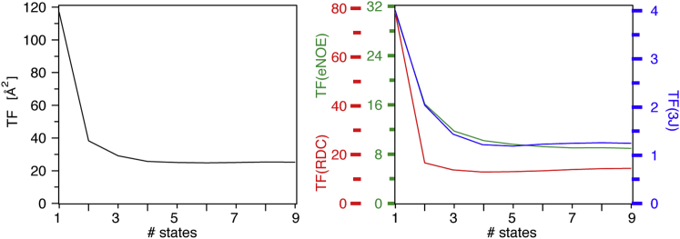
The CYANA target function is a measure of the violation of the experimental restraint data by the calculated structures. Thus, it may be used to estimate the appropriate number of states for representation of the spatial sampling of a molecule. The overall target function averaged over the 20 lowest-energy conformers of ∼117 Å² obtained for one state decreases to approximately one-third of its value for two states (Fig. 1, left). Additional decrease is observed when going to three and four states, where it reaches a plateau value of ∼30 Å². Plots of the contributions to the target function from eNOEs, RDCs, and J couplings (Fig. 1, right) reveal that the RDCs account for the major part of the target-function value and also for the major part of the decrease from one to two states. The decrease from two to three and again to four states is dominated by the eNOEs, whose target-function value continues to drop slightly up to nine states. The J couplings have a similar profile as the eNOEs, but their target function reaches the minimum at four states.

Figure 1.

Target function values obtained from multistate ensemble determination of GB3. The overall target function value is shown on the left, and the contributions from eNOEs, RDCs, and J couplings on the right. To see this figure in color, go online.

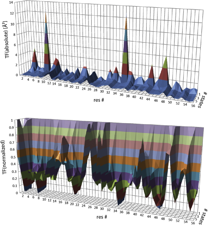
To understand the origins of major contributions to the target function, we calculated the residue-specific target-function values of the complete eNOE, J-coupling, and RDC data set (Fig. 2). The largest contributions to the target functions of the single-state structure stem from residues 8 and 35 (>12 Å²; Fig. 2, top). Those from residues 3, 11, 32, 43, 46, and 47 are also >3 Å². All of them undergo a dramatic decrease upon addition of a second state. As a consequence, these residues also undergo the largest decreases of the relative contributions normalized to the single-state contributions (Fig. 2, bottom). To check whether the large contributions are a simple consequence of a large number of restraints on the residue, the individual contributions were divided by the number of restraints per residue, as shown in Fig. S1. The profile is very similar to the one that is not normalized. The largest values are observed for residues 3, 8, 11, 22, 35, and 47 (>0.05 Å²). If the number of restraints has an impact, it is only exerted in an indirect manner, where the requirement to satisfy all restraints simultaneously drives the violation of each restraint up.

Figure 2.

Residue-specific target function values (TF). The individual contributions are plotted versus the residue number and the number of states on the x and y axes, respectively. The target function values are shown in absolute values (top) and normalized to the values for the single-state structure (bottom). To see this figure in color, go online.

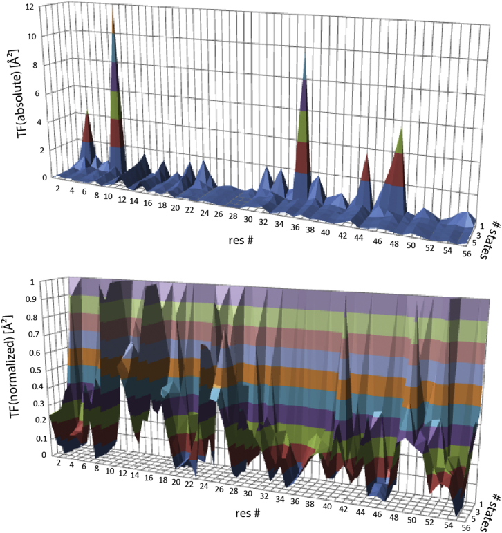
To further dissect the residue-specific contributions to the target function, we divided them up into the contributions from the backbone and the side chains (see Figs. 3 and S2). It is striking that the profile of the target-function values from the side chains is similar to that of the total residue-specific target-function values (compare Figs. 2 and 3). Thus, the large violations are mainly caused in the side chains. Indeed, the two most violated residues, 8 and 35, are known to simultaneously populate two χ¹ rotamer states (43). As most side-chain restraints of our data set strongly depend on the χ¹ angle, it is expected that single-state structures cannot fulfill the experimental data well. However, one additional state enables population of both rotameric states and the target-function values undergo a dramatic decrease (see normalized target-function values). It appears to be a consequence of the large violations in the side chains that some of the elevated target function values are also observed in the backbone, as the same residues have the largest values (see Fig. S2).

Figure 3.

Contributions to residue-specific target function values from the side chains. The individual contributions are plotted versus the residue number and the number of states on the x and y axes, respectively. The target function values are shown in absolute values (top) and normalized to the values for the single-state structure (bottom). To see this figure in color, go online.

Other segments that have larger-than-usual contributions to the target function are the highly mobile loop of residues 9–12, and also residues 43–47 in β-strand 3, which has been shown to be more mobile than the other strands (42). These residues also experience a large relative decrease of the individual target function values upon addition of further states. This indicates that the violations can be resolved with multiple states.

Although the overall target-function value is not reduced substantially when going from three to four states, the overall eNOE target function drops continuously over up to nine states, and the J-coupling target function clearly reaches the minimum at four states. Some residue-specific target-function values are reduced significantly when going to four, five, or six states. Because we wish to represent local conformational sampling appropriately rather than only globally, we choose four states for the appropriate ensemble representation in the following.

Interestingly, the optimal number of structural states to represent a set of NMR and x-ray observables obtained from GB3 was also shown to be four in a previous study (10). In that study, RDCs, Lipari-Szabo-type order parameters as determined from relaxation measurements, and crystallographic B-factors were used for ensemble calculation. Cross-validation was done with ³J_HN,Hα scalar couplings and backbone RDCs. Substantial improvement was observed when going from one to two states, and some more for four states. Depending on the observables, further slight improvement was achieved with 8 or 16 states. The input data set was smaller than ours, but the information content is difficult to compare to that of our set because of the very different nature of some of the data. In a prior study of GB3 by the same authors, based only on RDCs, the optimal number of states was two (17).

Structural ensembles

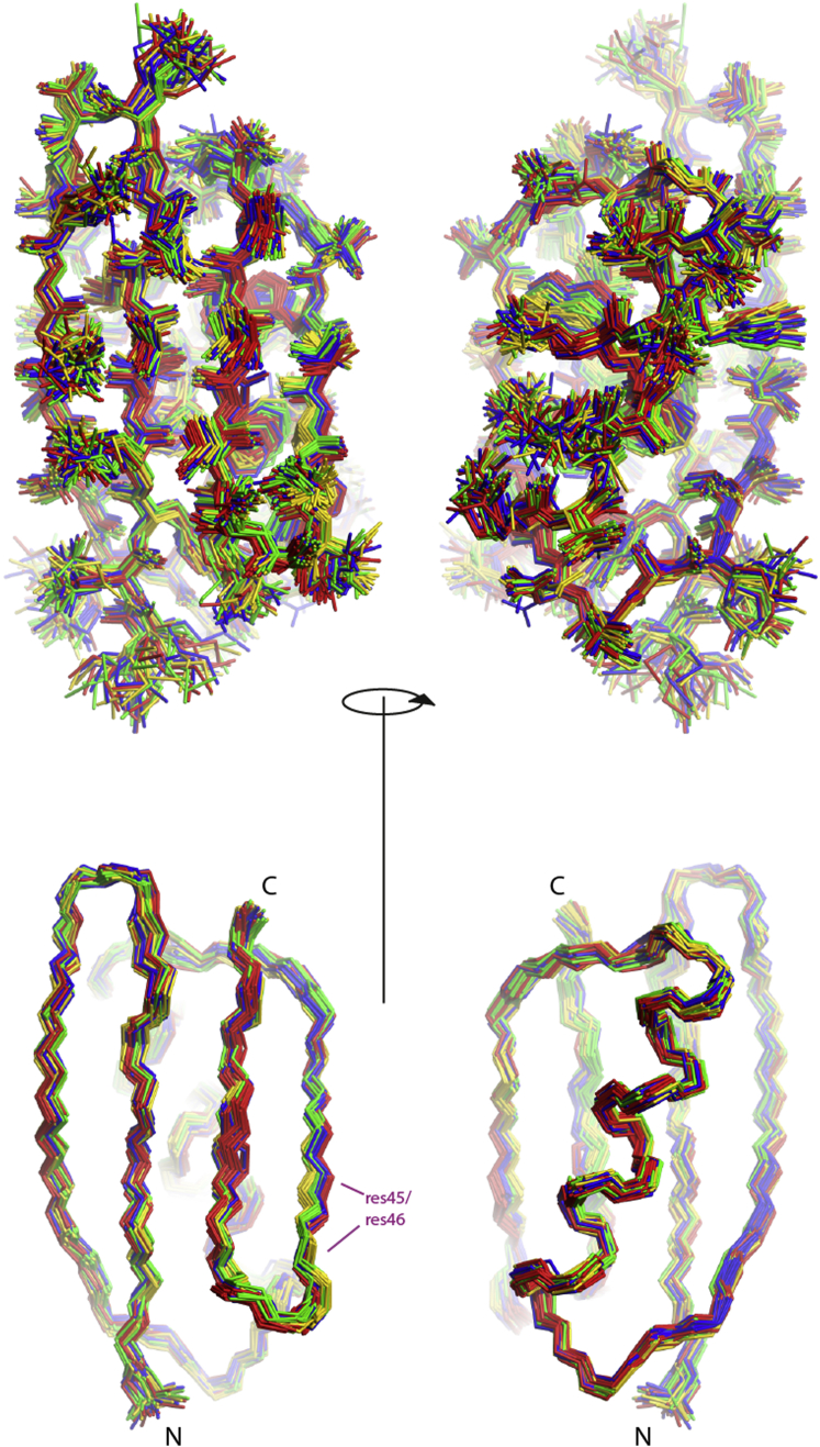
For the structural representation of GB3, we select the 20 four-state ensembles with the lowest target-function values from 100 calculations (Table 1). The ensembles are very compact, as expected for a highly rigid globular protein (Figs. 4 and 5). The squared H^N-N order parameters are 0.77 on average, and the root mean-square deviations (RMSDs) from the mean coordinates are 0.45 Å and 0.88 Å for the backbone and all heavy atoms, respectively. The RMSDs from an RDC-refined high-resolution x-ray structure are 0.55 Å and 1.09 Å for the backbone and all heavy atoms, respectively (41, 42, 45). For comparison, the previously published three-state structure obtained from a slightly smaller number of eNOEs and small RDC and J-coupling sets had RMSDs from the mean of 0.47 Å and 0.86 Å for the backbone and all heavy atoms, respectively, and RMSDs from the RDC-refined x-ray structure of 0.72 Å and 1.31 Å (35, 36). This indicates that the extended input data set does not alter the amplitude of the spatial sampling. Nevertheless, the four-state ensembles have a smaller deviation from the reference structure.

Table 1.

Structural Statistics for GB3

Parameters	eNOE-Derived Four-State Ensemble-Based Calculation	eNOE-Derived Three-State Ensemble-Based Calculationa
Restraints
Upper distance limits	984	884
Bidirectional	355	324
Unidirectional	568	481
Aromatics	61	61
Lower distance limits	923	823
Bidirectional	355	324
Unidirectional	568	481
Dihedral angles	–b	54
3J couplings	225	147
Backbone	147	147
Backbone-side-chain	78	–
RDCs	1477	90
Backbone	1335	90
Backbone-side-chain	13	–
Side chain	129	–
Average target-function value (Å2)	25.03	9.94
Violations
Distance restraints (>0.5 Å)	2	2
Torsion angle restraints (>5°)	–b	1
J-coupling restraints (>1 Hz)	5	3
RDC restraints (>4 Hz)	8	1
RDC restraints (>10% of range)	31 (5; 1; 19; 5; 1)c	3
Average RMSD from mean coordinates (Å)
Backbone atoms	0.45 ± 0.04	0.47 ± 0.05
Heavy atoms	0.88 ± 0.04	0.86 ± 0.04
RMSD from RDC-refined x-ray structured (Å)
Backbone atoms	0.55	0.72
Heavy atoms	1.09	1.31

^aThree-state ensemble-based calculations were taken from Yao et al. (41, 42) and Derrick and Wigley (45).

^bTorsion-angle restraints were turned off during the final stage of the calculation.

^cH^N-N, 3 Hz; H^α-C^α, H^β(2,3)-C^β, and H^β2-H^β3, 6 Hz; C^α-C′ and H^α-C^β, 0.7 Hz; H^N-C′, 1.2 Hz; C^x-C^methyl, 1 Hz.

^dRMSD values for eNOE calculations were taken from our previous work (35).

Figure 4.

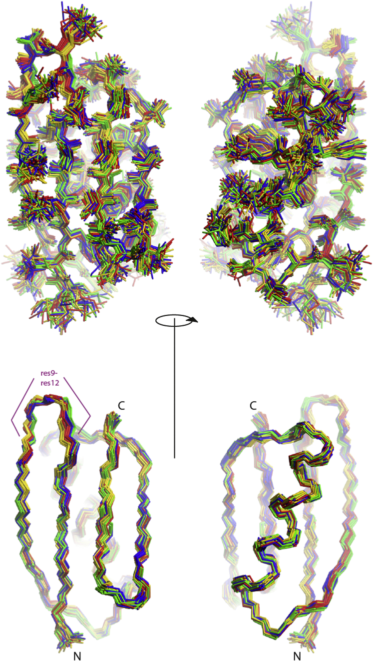
Four-state ensembles of GB3, showing the heavy-atom representations (top) and the backbone heavy-atom representations (bottom). The 20 ensembles with the lowest target-function values are selected and the four states colored gold, red, green, and blue are obtained by grouping the loop comprising residues 9–12. To see this figure in color, go online.

Figure 5.

Four-state ensembles of GB3, showing heavy-atom representations (top) and backbone heavy-atom representations (bottom). The 20 ensembles with the lowest target-function values are selected and the four states colored gold, red, green, and blue are obtained by grouping residues 45 and 46. To see this figure in color, go online.

In many structural segments, it is possible to manually identify the identical four states in all 20 ensembles. Apparently, some properties of the four obtained states are well defined by the input data in combination with the geometric constraints. In Figs. 4 and 5, the states were colored according to the segments comprising residues 9–12 and 45–46, respectively. Patterns of strong correlations in the immediate surroundings of these segments are present, but there are also long-range correlations within the β-sheet. To a lesser degree, the α-helix is also correlated with segment 45–46.

Information content of data sets

The very high density of eNOE, RDC, and J-coupling restraints is an excellent prerequisite to study the information content of these data. We wish to investigate the following. First, how much additional information is provided by RDCs and J couplings once the eNOE data set is collected? Second, how many additional data are provided by eNOEs when they replace a set of conventional NOEs? The first question is highly relevant for practical considerations, because it is a substantially smaller effort to collect an eNOE data set than the RDCs under multiple alignment conditions and J couplings. In practice, the preparation of eight alignment conditions is prohibitive for most systems, if it is possible at all (58). The second question is interesting in so much as the collection of an eNOE data set requires around four to five times more spectrometer time than conventional NOEs.

Backbone dihedral angles

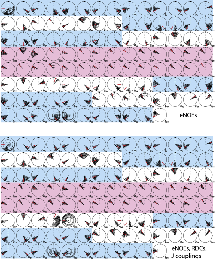
First, we investigated the impact on the backbone dihedral angles, φ and ψ, of supplementing the eNOE data with RDCs and J couplings. To that end, we plotted circle diagrams of φ and ψ sampled in four-state ensembles calculated from eNOEs only or from eNOEs, RDCs, and J couplings (see Fig. 6). The mean angles and the sampling are very similar in any kind of ensemble once eNOEs are employed (averaged over all residues, there is an 8.6° and 9.9° difference for the mean φ and ψ angles, respectively, whereas the standard deviation changes by −0.9° and +0.3° upon inclusion of the RDCs and J couplings, resulting in 16.1° and 17.3°). These relatively small changes are also reflected in minor changes of the backbone heavy-atom Cartesian RMSDs (from 0.47 Å to 0.45 Å). There are, however, some exceptions. Angles with increases of the standard deviation by >5° are ψ₇, ψ₉, φ₁₀, ψ₁₀, ψ₁₁, ψ₁₃, φ₁₅, ψ₁₆, ψ₂₄, φ₂₅, ψ₂₅, φ₂₆, ψ₃₈, φ₃₉, φ₄₀, φ₄₁, ψ₄₆, ψ₄₇, and φ₄₈, where the additional data apparently enforce a more distinct separation of states. None of the changes exceeds 20° except in the case of ψ₃₈ and φ₃₉ in the highly mobile loop comprised of residues 38–41, with +56.6° and +61.1°. Many of the more flexible angles are those of the four glycines at positions 9, 14, 38, and 41, which experience less steric hindrance due to the lack of a side chain. In both ensembles, the angles have generally a smaller standard deviation in the α-helix than in other secondary elements.

Figure 6.

Circle diagrams of backbone φ and ψ torsion angles. The four states of 20 ensembles are plotted from the center to the outer circle. Angles obtained from ensembles calculated from eNOEs exclusively are shown on the top, and ensembles calculated from eNOEs, RDCs, and J couplings on the bottom. The red bars indicate angles extracted from the high-resolution x-ray structure 1IGD (45). Diagrams of residues that are located in a β-strand and the α-helix are shaded in blue and pink, respectively. The figure was generated in MolMol (59). To see this figure in color, go online.

The angles of both ensembles also coincide very closely with those extracted from a high-resolution x-ray structure (45). Almost all x-ray-derived angles fall within the ranges sampled by the ensemble, the only exceptions being φ₂, φ₁₄, ψ₁₄, ψ₃₈, φ₃₉,ψ₄₀, and φ₄₁, all of which are located in the hinge regions of the two flexible loops or the N-terminus. Note, however, that the differences are small in all cases (<30°).

To see if a good definition of the ensemble is a general property of NOEs, we generated analogous plots for ensembles obtained from conventional NOEs with or without RDCs and J couplings (see Fig. S3). Here, the changes are significantly more pronounced. Although the means change only slightly more (15.8° and 17.1° for the φ and ψ angles, respectively), the standard deviations decrease by −11.2° and −10.3° upon inclusion of the RDCs and J couplings, resulting in 19.2° and 19.8°. First, this indicates that definition of the ensemble backbone by conventional NOEs is not as tight as that by eNOEs. This is also reflected in the overall backbone heavy-atom RMSD from the average of 0.77 Å of the ensembles obtained only from conventional NOEs. Furthermore, it demonstrates that even using the RDCs and J couplings, the backbone trace is not equally compact when conventional NOEs are used instead of eNOEs. Interestingly, this difference is not seen in the overall backbone heavy-atom RMSD that decreases to 0.43 Å, which is similar to what is seen for eNOE-based ensembles.

Side-chain χ¹ angles

Next, we investigate the impact of supplementing the eNOE data with RDCs and J couplings on the side chains. χ¹ dihedral angles are the ideal probes, because our data set contains a high density of RDCs and J-coupling restraints on χ¹. Although a single-state bundle calculation with eNOE restraints produces considerably smaller standard deviations from the mean values of χ¹ than one with conventional NOEs (averaged over all residues, the standard deviations are 19.6° versus 46.8°), the obtained rotamer states are identical in nearly all cases (see a circle diagram plot in Fig. S4). In the following, we investigate whether differences in the χ¹ means and standard deviations are obtained for the four-state ensembles calculated with different input data sets, where a higher information density is required.

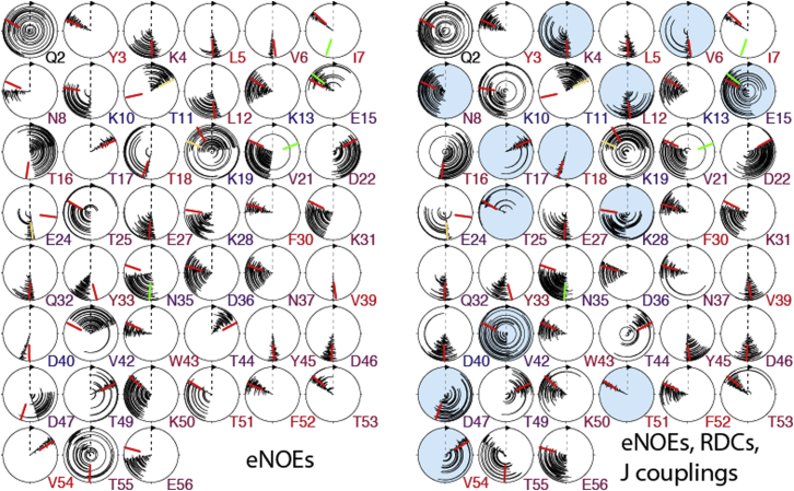
Fig. 7 shows a comparison of the χ¹ torsion angle sampling in the four-state ensembles calculated either from eNOEs only or from eNOEs, RDCs, and J couplings. On average, the complete data set changes the mean angles by 18.8° and the standard deviations by +7.7° for individual residues. These relatively small changes are similar to those observed for the backbone dihedral angles and are again reflected by minor changes of the overall heavy-atom RMSDs (from 0.83 Å to 0.88 Å). This observation indicates the high information content of the eNOE data set. However, some additional states appear, whereas others disappear, when RDCs and J couplings are added to the input data set. This is observed for about one-third of the χ¹ angles (residues 4, 6, 8, 12, 15, 17, 18, 25, 28, 42, 47, 51, and 54; Fig. 7, light blue circles). Angles extracted from high-resolution x-ray structures are also indicated (45). The few angles in the single-state structures from the conventional NOEs as well as the eNOEs that were not in agreement with the x-ray structure (see Fig. S4) have a significant population at the x-ray angles now. For residues 7 and 21, the original isotropic x-ray angle is in agreement with the ensemble value, but not the alternative state from anisotropic evaluation. For residues 11 and 24, the additional state is sampled, but not the isotropic one. For residue 35, both the original isotropic and the different states are sampled. Overall, there is a very good agreement between the NMR and x-ray data. Those non-alanine/glycine residues with a very low percentage of solvent-accessible surface area (<10% as calculated for the GB3 (PDB: 1IGD) (45) from MolMol with a solvent molecule of radius 1.4 Å (59)), residues 3, 5, 7, 30, 39, 52, and 54, have a single rotamer state with a very small standard deviation. For those with a higher percentage, no clear pattern emerges. For example, among the three residues with >50% solvent-accessible surface area, residue 40 has a narrow distribution, whereas residues 10 and 11 sample two states.

Figure 7.

Sufficiency of eNOEs in defining χ¹ angles. Angles obtained from ensembles calculated from eNOEs exclusively are shown on the left, and ensembles calculated from eNOEs, RDCs, and J couplings on the right. The four states of 20 ensembles are plotted from the center to the outer circle in the circle diagrams. The red bars indicate angles extracted from the high-resolution x-ray structure 1IGD (45), and the green and yellow bars different states and additional states from an anisotropic reevaluation. Angles for which an additional state is obtained or a state disappears are shaded in light blue. The single-letter amino acid codes and residue numbers are colored according to the solvent-accessible surface area of the residue (red for 0% and blue for 50% or more). The figure was generated in MolMol (59). To see this figure in color, go online.

We also compared the four-state ensemble calculated from eNOEs alone to the previously determined three-state ensemble based on a slightly smaller eNOE set but with 153 J couplings from the backbone and one H^N-N and one H^α-C^α RDC set (PDB: 2LUM) (35, 36). This ensemble yields results very similar to those of the four-state ensemble (see Fig. S5). Notable differences are only observed for residues 15 (minor population shifts from gauche+ (g+) to trans (tr)), 37 (slightly reduced minor state population), 42 (addition of tr state), 45 (less well defined), 50 (tr shifts to g+ rotamer), and 54 (addition of tr state). Interestingly, all these changes bring the ensemble closer to the four-state ensemble obtained from the complete data set.

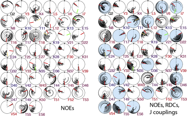
Fig. 8 shows a comparison analogous to the one in Fig. 7, where the eNOE set is replaced by the conventional NOE set. On average, the complete data set changes the mean angles by 33.8° and the standard deviations by +7.7° for individual residues. Again, some additional states appear, whereas others disappear. This is observed for approximately one-half of the angles, which is more than the one-third in the case of the eNOEs. These considerably larger changes compared to those for the eNOEs are also reflected in a relatively large change of overall heavy-atom Cartesian RMSDs (from 1.11 Å to 0.88 Å). Obviously, the RDC and J couplings contain more information that is not redundant with the NOEs than with the eNOEs.

Figure 8.

Sufficiency of conventional NOEs in defining χ¹ angles. Angles obtained from ensembles calculated from conventional NOEs exclusively are shown on the left, and ensembles calculated from conventional NOEs, RDCs, and J couplings on the right. The four states of 20 ensembles are plotted from the center to the outer circle in the circle diagrams. The red bars indicate angles extracted from the high-resolution x-ray structure 1IGD (45), and the green and yellow bars indicate different states and additional states from an anisotropic reevaluation. Angles for which an additional state is obtained or a state disappears are shaded in light blue. The single-letter amino acid codes and residue numbers are colored according to the solvent-accessible surface area of the residue (red for 0% and blue for 50% or more). The figure was generated in MolMol (59). To see this figure in color, go online.

The standard deviation of the eNOE-based angles is 3.5° smaller on average than those based on conventional NOEs. However, the residue-averaged change of the mean angles by 33.5° indicates that some states are different (compare Figs. 7, right, and 8, right). These may be grouped into the following categories. When going from conventional NOEs to eNOEs, we observe a new major state (residue 22, tr, and gauche− (g−)), loss of one or two minor states (residues 8, tr; 15, tr; 17, tr; 25, tr; 44, tr and g−; 47, g−), addition of a minor state (16, 0°; 21, tr), change of a minor state (10, g+ to tr; 19, tr to g+; 36, tr to g−; 42, tr to g+; 55, g− to g+), stronger distinction of two present states (12; 13; 31; 37), and narrower distributions (32; 40; 46; 53).

Structural correlations

Backbone and χ¹ dihedral angles

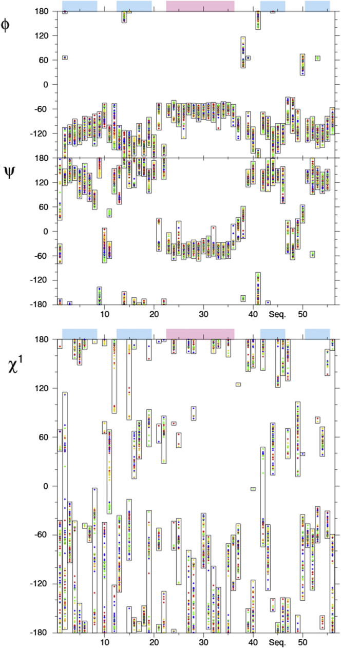
Multiple-state representations of molecular structures not only map motional amplitudes but can also reveal correlations between entities as they sample the conformational space. Here, we analyze the correlations in four-state ensembles for the φ, ψ, and χ¹ angles by bar plots of the states (see Figs. 9 and S6). The same color code as in Figs. 4 and 5 is used. Since manual grouping was carried out in the loop connecting β-strands 1 and 2, comprising residues 9–12 in the first case (Figs. 4 and 9), there is a high correlation between the identical states in the different ensembles in close proximity to this loop. This is particularly true for the ψ angles but is also propagated into the φ and χ¹ angles, and to a lesser degree into the peripheral side-chain angles χ², χ³, etc. For φ, ψ, and χ¹ (and even χ²), the correlation is somewhat conserved in the first two β-strands. Similar effects are observed when grouping residues 45 and 46 (see Figs. 5 and S6), where the highest correlation is present in the neighborhood of the corresponding residues. It is worth noting that one strength of the eNOE-based multistate ensemble is their sensitivity to translational correlations, in some cases of entire segments, rather than only angular correlations. Such correlations may be most easily visualized in the state representations of Figs. 4 and 5. In all ensembles, a strong correlation with the four states in the loop comprising residues 9–12 is present and propagates into β-strands 1, 2, and 4. When grouping the segment of residues 45 and 46, the correlations are strongest in the adjacent strands 3 and 4, but are present in the entire β sheet. To a lesser extent, the correlations also propagate into the α-helix.

Figure 9.

Correlations in four-state ensembles of GB3 calculated from eNOEs, RDCs, and J couplings. Shown are φ (top), ψ (middle), and χ¹ angles (bottom). The states are grouped in the loop comprising residues 9–12 and the colors are the same as in Fig. 4. β-strands and the α-helix are indicated by blue and pink shading, respectively, above the plots. The figure was generated in MolMol (59). To see this figure in color, go online

Principal component analysis

A more quantitative way to analyze the states in multiple-state ensembles may be by principal component analysis (PCA) (35, 60). We applied PCA to the 20 four-state ensembles (see Materials and Methods). Fig. S7 shows the 10 largest principal components. When the 20 four-state ensembles are projected into the first two principal components, they divide into groups with the 20 lowest (most negative), second lowest, second largest, and 20 largest (most positive) values for both principal components, and the four states per ensemble end up in the four different groups in most cases (Fig. S8). This indicates that the choice of four states in the ensemble calculation is not producing redundant structural representations. This double grouping along the first two principal components captures the two main spatial sampling features that are not correlated with each other. Interestingly, the principal modes do not coincide with the highly localized manual grouping of either the loop comprising residues 9–12 or the segment with residues 45 and 46. Instead, the modes reveal more subtle features distributed over the entire protein.

Conclusions

We have analyzed the information content of an extended eNOE data set of GB3 with respect to large sets of RDCs obtained under eight alignment conditions and J couplings defining backbone φ and side-chain χ¹ angles. To this purpose, we modified our previously established protocol for multiple-state ensemble determination to determine four-state ensembles of GB3. We justified the choice of four states by dissecting the contributions to the CYANA target function and by PCA. By omitting subsets of the input data in the structure calculation, we show that 1), eNOE distance restraints contain more information than those derived from conventional NOEs, and 2) eNOEs alone, as opposed to conventional NOEs, provide state representations similar to those of the complete input data set including the RDCs and J couplings.

These insights are of immediate significance, because the experimental effort to obtain eNOEs is substantially smaller than that required to collect RDCs under multiple alignment conditions and J couplings. In addition, we conclude that it is worth replacing conventional NOEs with eNOEs in structural analysis. The additional effort is minimal. The NOESY assignment has to be carried out only once in both cases. The more sophisticated evaluation procedure of eNOEs is largely automated in our latest software versions (to be published elsewhere). We believe that the four to five times longer measurement time is easily compensated for by the gain in information and the saved experimental effort (RDCs, J couplings).

Our method for multistate ensemble determination can be easily applied to other systems with masses up to 20 kDa. For example, we recently determined two states of cyclophilin A, an enzyme of 18 kDa (61). In one state, the binding loop is closed, whereas it is open in the other state while the active site is preorganized for ligand binding. As the NOE is sensitive to motions on timescales as slow as milliseconds, we expect the method to reveal further biologically relevant mechansims when applied to other proteins or nucleic acids.

Finally, the compiled data set consisting of eNOEs, RDCs, and J coupling of GB3 is one of the largest, most accurate, and most diverse for any protein. Therefore, we advocate this set to be an ideal test case for methods development in molecular dynamics simulations and structure calculations.

Author Contributions

B.V., S.O., P.G., and R.R. designed research; B.V., S.O., and P.G. performed research, analyzed data, and wrote the article.

Editor: Jeff Peng.

References

- 1.Gibbs A.C. Elements and modulation of functional dynamics. J. Med. Chem. 2014;57:7819–7837. doi: 10.1021/jm500325k. [DOI] [PubMed] [Google Scholar]
- 2.van den Bedem H., Fraser J.S. Integrative, dynamic structural biology at atomic resolution—it’s about time. Nat. Methods. 2015;12:307–318. doi: 10.1038/nmeth.3324. [DOI] [PMC free article] [PubMed] [Google Scholar]
- 3.Lipari G., Szabo A. Model-free approach to the interpretation of nuclear magnetic resonance relaxation in macromolecules. 1. Theory and range of validity. J. Am. Chem. Soc. 1982;104:4546–4559. [Google Scholar]
- 4.Kay L.E., Torchia D.A., Bax A. Backbone dynamics of proteins as studied by 15N inverse detected heteronuclear NMR spectroscopy: application to staphylococcal nuclease. Biochemistry. 1989;28:8972–8979. doi: 10.1021/bi00449a003. [DOI] [PubMed] [Google Scholar]
- 5.Meiler J., Prompers J.J., Brüschweiler R. Model-free approach to the dynamic interpretation of residual dipolar couplings in globular proteins. J. Am. Chem. Soc. 2001;123:6098–6107. doi: 10.1021/ja010002z. [DOI] [PubMed] [Google Scholar]
- 6.Salmon L., Bouvignies G., Blackledge M. Nuclear magnetic resonance provides a quantitative description of protein conformational flexibility on physiologically important time scales. Biochemistry. 2011;50:2735–2747. doi: 10.1021/bi200177v. [DOI] [PubMed] [Google Scholar]
- 7.Fenwick R.B., Esteban-Martín S., Salvatella X. Understanding biomolecular motion, recognition, and allostery by use of conformational ensembles. Eur. Biophys. J. 2011;40:1339–1355. doi: 10.1007/s00249-011-0754-8. [DOI] [PMC free article] [PubMed] [Google Scholar]
- 8.Ángyán A.F., Gáspári Z. Ensemble-based interpretations of NMR structural data to describe protein internal dynamics. Molecules. 2013;18:10548–10567. doi: 10.3390/molecules180910548. [DOI] [PMC free article] [PubMed] [Google Scholar]
- 9.Bouvignies G., Bernadó P., Blackledge M. Identification of slow correlated motions in proteins using residual dipolar and hydrogen-bond scalar couplings. Proc. Natl. Acad. Sci. USA. 2005;102:13885–13890. doi: 10.1073/pnas.0505129102. [DOI] [PMC free article] [PubMed] [Google Scholar]
- 10.Clore G.M., Schwieters C.D. Concordance of residual dipolar couplings, backbone order parameters and crystallographic B-factors for a small α/β protein: a unified picture of high probability, fast atomic motions in proteins. J. Mol. Biol. 2006;355:879–886. doi: 10.1016/j.jmb.2005.11.042. [DOI] [PubMed] [Google Scholar]
- 11.Lange O.F., Lakomek N.-A., de Groot B.L. Recognition dynamics up to microseconds revealed from an RDC-derived ubiquitin ensemble in solution. Science. 2008;320:1471–1475. doi: 10.1126/science.1157092. [DOI] [PubMed] [Google Scholar]
- 12.Fenwick R.B., Esteban-Martín S., Salvatella X. Weak long-range correlated motions in a surface patch of ubiquitin involved in molecular recognition. J. Am. Chem. Soc. 2011;133:10336–10339. doi: 10.1021/ja200461n. [DOI] [PMC free article] [PubMed] [Google Scholar]
- 13.Berlin K., Castañeda C.A., Fushman D. Recovering a representative conformational ensemble from underdetermined macromolecular structural data. J. Am. Chem. Soc. 2013;135:16595–16609. doi: 10.1021/ja4083717. [DOI] [PMC free article] [PubMed] [Google Scholar]
- 14.Olsson S., Vögeli B.R., Hamelryck T. Probabilistic determination of native state ensembles of proteins. J. Chem. Theory Comput. 2014;10:3484–3491. doi: 10.1021/ct5001236. [DOI] [PubMed] [Google Scholar]
- 15.Olsson S., Ekonomiuk D., Cavalli A. Molecular dynamics of biomolecules through direct analysis of dipolar couplings. J. Am. Chem. Soc. 2015;137:6270–6278. doi: 10.1021/jacs.5b01289. [DOI] [PubMed] [Google Scholar]
- 16.Clore G.M., Schwieters C.D. How much backbone motion in ubiquitin is required to account for dipolar coupling data measured in multiple alignment media as assessed by independent cross-validation? J. Am. Chem. Soc. 2004;126:2923–2938. doi: 10.1021/ja0386804. [DOI] [PubMed] [Google Scholar]
- 17.Clore G.M., Schwieters C.D. Amplitudes of protein backbone dynamics and correlated motions in a small α/β protein: correspondence of dipolar coupling and heteronuclear relaxation measurements. Biochemistry. 2004;43:10678–10691. doi: 10.1021/bi049357w. [DOI] [PubMed] [Google Scholar]
- 18.Clore G.M., Iwahara J. Theory, practice, and applications of paramagnetic relaxation enhancement for the characterization of transient low-population states of biological macromolecules and their complexes. Chem. Rev. 2009;109:4108–4139. doi: 10.1021/cr900033p. [DOI] [PMC free article] [PubMed] [Google Scholar]
- 19.Russo L., Maestre-Martinez M., Griesinger C. Interdomain dynamics explored by paramagnetic NMR. J. Am. Chem. Soc. 2013;135:17111–17120. doi: 10.1021/ja408143f. [DOI] [PubMed] [Google Scholar]
- 20.Brüschweiler R., Blackledge M., Ernst R.R. Multi-conformational peptide dynamics derived from NMR data: a new search algorithm and its application to antamanide. J. Biomol. NMR. 1991;1:3–11. doi: 10.1007/BF01874565. [DOI] [PubMed] [Google Scholar]
- 21.Lindorff-Larsen K., Best R.B., Vendruscolo M. Simultaneous determination of protein structure and dynamics. Nature. 2005;433:128–132. doi: 10.1038/nature03199. [DOI] [PubMed] [Google Scholar]
- 22.Richter B., Gsponer J., Vendruscolo M. The MUMO (minimal under-restraining minimal over-restraining) method for the determination of native state ensembles of proteins. J. Biomol. NMR. 2007;37:117–135. doi: 10.1007/s10858-006-9117-7. [DOI] [PubMed] [Google Scholar]
- 23.Hyberts S.G., Goldberg M.S., Wagner G. The solution structure of eglin c based on measurements of many NOEs and coupling constants and its comparison with x-ray structures. Protein Sci. 1992;1:736–751. doi: 10.1002/pro.5560010606. [DOI] [PMC free article] [PubMed] [Google Scholar]
- 24.Lindorff-Larsen K., Best R.B., Vendruscolo M. Interpreting dynamically-averaged scalar couplings in proteins. J. Biomol. NMR. 2005;32:273–280. doi: 10.1007/s10858-005-8873-0. [DOI] [PubMed] [Google Scholar]
- 25.Robustelli P., Kohlhoff K., Vendruscolo M. Using NMR chemical shifts as structural restraints in molecular dynamics simulations of proteins. Structure. 2010;18:923–933. doi: 10.1016/j.str.2010.04.016. [DOI] [PubMed] [Google Scholar]
- 26.Camilloni C., Cavalli A., Vendruscolo M. Assessment of the use of NMR chemical shifts as replica-averaged structural restraints in molecular dynamics simulations to characterize the dynamics of proteins. J. Phys. Chem. B. 2013;117:1838–1843. doi: 10.1021/jp3106666. [DOI] [PubMed] [Google Scholar]
- 27.Vögeli B., Orts J., Riek R. Discrete three-dimensional representation of macromolecular motion from eNOE-based ensemble calculation. Chimia (Aarau) 2012;66:787–790. doi: 10.2533/chimia.2012.787. [DOI] [PubMed] [Google Scholar]
- 28.Vögeli B., Orts J., Riek R. Towards a true protein movie: a perspective on the potential impact of the ensemble-based structure determination using exact NOEs. J. Magn. Reson. 2014;241:53–59. doi: 10.1016/j.jmr.2013.11.016. [DOI] [PubMed] [Google Scholar]
- 29.Vögeli B. The nuclear Overhauser effect from a quantitative perspective. Prog. Nucl. Magn. Reson. Spectrosc. 2014;78:1–46. doi: 10.1016/j.pnmrs.2013.11.001. [DOI] [PubMed] [Google Scholar]
- 30.Keepers J.W., James T.L. Theoretical study of distance determinations from NMR. Two-dimensional nuclear Overhauser effect spectra. J. Magn. Reson. 1984;57:404–426. [Google Scholar]
- 31.Boelens R., Koning T.M.G., Kaptein R. Determination of biomolecular structures from proton-proton NOE’s using a relaxation matrix approach. J. Mol. Struct. 1988;173:299–311. [Google Scholar]
- 32.Boelens R., Koning T.M.G., Kaptein R. Iterative procedure for structure determination from proton-proton NOEs using a full relaxation matrix approach. Application to a DNA octamer. J. Magn. Reson. 1969;82:290–308. [Google Scholar]
- 33.Vögeli B., Segawa T.F., Riek R. Exact distances and internal dynamics of perdeuterated ubiquitin from NOE buildups. J. Am. Chem. Soc. 2009;131:17215–17225. doi: 10.1021/ja905366h. [DOI] [PubMed] [Google Scholar]
- 34.Vögeli B., Friedmann M., Riek R. Quantitative determination of NOE rates in perdeuterated and protonated proteins: practical and theoretical aspects. J. Magn. Reson. 2010;204:290–302. doi: 10.1016/j.jmr.2010.03.009. [DOI] [PubMed] [Google Scholar]
- 35.Vögeli B., Kazemi S., Riek R. Spatial elucidation of motion in proteins by ensemble-based structure calculation using exact NOEs. Nat. Struct. Mol. Biol. 2012;19:1053–1057. doi: 10.1038/nsmb.2355. [DOI] [PubMed] [Google Scholar]
- 36.Vögeli B., Güntert P., Riek R. Multiple-state ensemble structure determination from eNOE spectroscopy. Mol. Phys. 2013;111:437–454. [Google Scholar]
- 37.Vögeli B., Olsson S., Güntert P. Complementarity and congruence between exact NOEs and traditional NMR probes for spatial decoding of protein dynamics. J. Struct. Biol. 2015;191:306–317. doi: 10.1016/j.jsb.2015.07.008. [DOI] [PubMed] [Google Scholar]
- 38.Vögeli B., Olsson S., Güntert P. Compiled data set of exact NOE distance limits, residual dipolar couplings and scalar couplings for the protein GB3. Data Brief. 2015;5:99–106. doi: 10.1016/j.dib.2015.08.020. [DOI] [PMC free article] [PubMed] [Google Scholar]
- 39.Strotz D., Orts J., Vögeli B. The experimental accuracy of the uni-directional exact NOE. J. Magn. Reson. 2015;259:32–46. doi: 10.1016/j.jmr.2015.07.007. [DOI] [PubMed] [Google Scholar]
- 40.Vögeli B., Yao L., Bax A. Protein backbone motions viewed by intraresidue and sequential HN-Hα residual dipolar couplings. J. Biomol. NMR. 2008;41:17–28. doi: 10.1007/s10858-008-9237-3. [DOI] [PMC free article] [PubMed] [Google Scholar]
- 41.Yao L., Vögeli B., Bax A. NMR determination of amide N-H equilibrium bond length from concerted dipolar coupling measurements. J. Am. Chem. Soc. 2008;130:16518–16520. doi: 10.1021/ja805654f. [DOI] [PMC free article] [PubMed] [Google Scholar]
- 42.Yao L., Vögeli B., Bax A. Simultaneous NMR study of protein structure and dynamics using conservative mutagenesis. J. Phys. Chem. B. 2008;112:6045–6056. doi: 10.1021/jp0772124. [DOI] [PubMed] [Google Scholar]
- 43.Miclet E., Boisbouvier J., Bax A. Measurement of eight scalar and dipolar couplings for methine-methylene pairs in proteins and nucleic acids. J. Biomol. NMR. 2005;31:201–216. doi: 10.1007/s10858-005-0175-z. [DOI] [PubMed] [Google Scholar]
- 44.Ottiger M., Bax A. How tetrahedral are methyl groups in proteins? A liquid crystal NMR study. J. Am. Chem. Soc. 1999;121:4690–4695. [Google Scholar]
- 45.Derrick J.P., Wigley D.B. The third IgG-binding domain from streptococcal protein G. An analysis by x-ray crystallography of the structure alone and in a complex with Fab. J. Mol. Biol. 1994;243:906–918. doi: 10.1006/jmbi.1994.1691. [DOI] [PubMed] [Google Scholar]
- 46.Vögeli B., Ying J., Bax A. Limits on variations in protein backbone dynamics from precise measurements of scalar couplings. J. Am. Chem. Soc. 2007;129:9377–9385. doi: 10.1021/ja070324o. [DOI] [PubMed] [Google Scholar]
- 47.Wang B., He X., Merz K.M. Quantum mechanical study of vicinal J spin-spin coupling constants for the protein backbone. J. Chem. Theory Comput. 2013;9:4653–4659. doi: 10.1021/ct400631b. [DOI] [PubMed] [Google Scholar]
- 48.Pérez C., Löhr F., Schmidt J.M. Self-consistent Karplus parametrization of 3J couplings depending on the polypeptide side-chain torsion χ1. J. Am. Chem. Soc. 2001;123:7081–7093. doi: 10.1021/ja003724j. [DOI] [PubMed] [Google Scholar]
- 49.Hu J.S., Grzesiek S., Bax A. Two-dimensional NMR methods for determining χ1 angles of aromatic residues in proteins from three-bond JCCγ and JNCγ couplings. J. Am. Chem. Soc. 1997;119:1803–1804. [Google Scholar]
- 50.Chou J.J., Case D.A., Bax A. Insights into the mobility of methyl-bearing side chains in proteins from 3JCC and 3JCN couplings. J. Am. Chem. Soc. 2003;125:8959–8966. doi: 10.1021/ja029972s. [DOI] [PubMed] [Google Scholar]
- 51.Chi C.N., Strotz D., Vögeli B. Extending the eNOE data set of large proteins by evaluation of NOEs with unresolved diagonals. J. Biomol. NMR. 2015;62:63–69. doi: 10.1007/s10858-015-9917-8. [DOI] [PubMed] [Google Scholar]
- 52.Orts J., Vögeli B., Güntert P. Stereospecific assignments in proteins using exact NOEs. J. Biomol. NMR. 2013;57:211–218. doi: 10.1007/s10858-013-9780-4. [DOI] [PubMed] [Google Scholar]
- 53.Güntert P. Automated NMR protein structure calculation. Prog. Nucl. Magn. Reson. Spectrosc. 2003;43:105–125. [Google Scholar]
- 54.Güntert P. Automated structure determination from NMR spectra. Eur. Biophys. J. 2009;38:129–143. doi: 10.1007/s00249-008-0367-z. [DOI] [PubMed] [Google Scholar]
- 55.Fletcher C.M., Jones D.N.M., Neuhaus D. Treatment of NOE constraints involving equivalent or nonstereoassigned protons in calculations of biomacromolecular structures. J. Biomol. NMR. 1996;8:292–310. doi: 10.1007/BF00410328. [DOI] [PubMed] [Google Scholar]
- 56.Brünger A.T., Clore G.M., Nilges M. Assessing the quality of solution nuclear magnetic resonance structures by complete cross-validation. Science. 1993;261:328–331. doi: 10.1126/science.8332897. [DOI] [PubMed] [Google Scholar]
- 57.Güntert P., Buchner L. Combined automated NOE assignment and structure calculation with CYANA. J. Biomol. NMR. 2015;62:453–471. doi: 10.1007/s10858-015-9924-9. [DOI] [PubMed] [Google Scholar]
- 58.Higman V.A., Boyd J., Redfield C. Residual dipolar couplings: are multiple independent alignments always possible? J. Biomol. NMR. 2011;49:53–60. doi: 10.1007/s10858-010-9457-1. [DOI] [PMC free article] [PubMed] [Google Scholar]
- 59.Koradi R., Billeter M., Wüthrich K. MOLMOL: a program for display and analysis of macromolecular structures. J. Mol. Graph. 1996;14:51–55. doi: 10.1016/0263-7855(96)00009-4. 29–32. [DOI] [PubMed] [Google Scholar]
- 60.Bahar I., Lezon T.R., Shrivastava I.H. Normal mode analysis of biomolecular structures: functional mechanisms of membrane proteins. Chem. Rev. 2010;110:1463–1497. doi: 10.1021/cr900095e. [DOI] [PMC free article] [PubMed] [Google Scholar]
- 61.Chi C.N., Vögeli B., Riek R. A structural ensemble for the enzyme cyclophilin reveals an orchestrated mode of action at atomic resolution. Angew. Chem. Int. Ed. Engl. 2015;54:11657–11661. doi: 10.1002/anie.201503698. [DOI] [PubMed] [Google Scholar]
Associated Data
This section collects any data citations, data availability statements, or supplementary materials included in this article.