Experimental Validation of Plastic Mandible Models Produced by a “Low-Cost” 3-Dimensional Fused Deposition Modeling Printer

Abstract

Background

The objective of this study was to investigate the accuracy of 3-dimensional (3D) plastic (ABS) models generated using a low-cost 3D fused deposition modelling printer.

Material/Methods

Two human dry mandibles were scanned with a cone beam computed tomography (CBCT) Accuitomo device. Preprocessing consisted of 3D reconstruction with Maxilim software and STL file repair with Netfabb software. Then, the data were used to print 2 plastic replicas with a low-cost 3D fused deposition modeling printer (Up plus 2^®). Two independent observers performed the identification of 26 anatomic landmarks on the 4 mandibles (2 dry and 2 replicas) with a 3D measuring arm. Each observer repeated the identifications 20 times. The comparison between the dry and plastic mandibles was based on 13 distances: 8 distances less than 12 mm and 5 distances greater than 12 mm.

Results

The mean absolute difference (MAD) was 0.37 mm, and the mean dimensional error (MDE) was 3.76%. The MDE decreased to 0.93% for distances greater than 12 mm.

Conclusions

Plastic models generated using the low-cost 3D printer UPplus2^® provide dimensional accuracies comparable to other well-established rapid prototyping technologies.

Validated low-cost 3D printers could represent a step toward the better accessibility of rapid prototyping technologies in the medical field.

Background

Rapid prototyping (RP) models obtained by additive manufacturing, which were initially described in the 1990s by Mankovich [1], are based on medical imaging (CT scans, CBCT, MRI, ultrasounds) and represent portions of human anatomy at a scale of 1:1 [2]. The 4 major RP technologies are stereolithography (SL), selective laser sintering (SLS), 3-dimensional printing (3DP), and fused deposition modelling (FDM) [3,4]. The current expansion of low-cost 3-dimensional (3D) printers is related to a recent transfer of RP patents into the public domain. As a result, more than 150 companies currently offer different types of low-cost 3D printers. The most commonly used thermoplastic materials in FDM technology are acrylonitrile butadiene styrene (ABS) and polylactic acid (PLA) filaments. Petropolis et al. [5] tested the accuracy of Cube 3D (3D Systems, Rock Hill, USA), which is a low-cost FDM printer using PLA as a thermoplastic raw material. Three 3D models of a skull and mandible were manufactured using 0.1 mm, 0.25 mm, and 0.50 mm layer heights [5]. A reference 3D model was also made with an industrial SLS printer for comparison [5]. Seven distances (5 distances on the skull and 2 transversal bony distances on the mandible) were measured by 1 observer 20 times with an electronic calliper [5]. Petropolis et al. [5] found that a dimensional error of 0.30% was observed for the SLS models and 0.44%, 0.52% and 1.1% for the 0.1 mm, 0.25 mm and 0.5 mm FDM models, respectively [5]. The authors warned about the use of ABS material as it may have some warping. However, this conclusion was not based on any experimental test but only on a literature reference from a textbook. On the other hand, Ernoult et al. [6] used a low-cost 3D printer (Up plus 2, Beijing, China) and ABS filament to manufacture 3 anatomic models and used them in 3 maxillofacial surgical cases. However, this case series article presenting clinical applications of a new technology failed to provide any: 1) ethics committee approval and informed patient consent obtained or 2) experimental validation and measurement of mean dimensional error (MDE) of 3D printed models [6].

Low-cost 3D printers need to be validated before they can be safely used in any medical applications. The first step of such validation requires testing of the accuracy of 3D models generated by low-cost 3D printers. Therefore, the aim of our study was to evaluate the accuracy of ABS models produced by a low-cost 3D FDM printer UPplus2^® by comparing the measurements obtained using original dry human mandibles with those of plastic replicas. Our hypothesis was that the accuracy of the 3D plastic replicas from a low-cost 3D FDM printer would be clinically acceptable. We also postulated that no warping would be present with Up plus 2 3D printed models.

Material and Methods

The overall methodological procedure is depicted in Figure 1.

Figure 1.

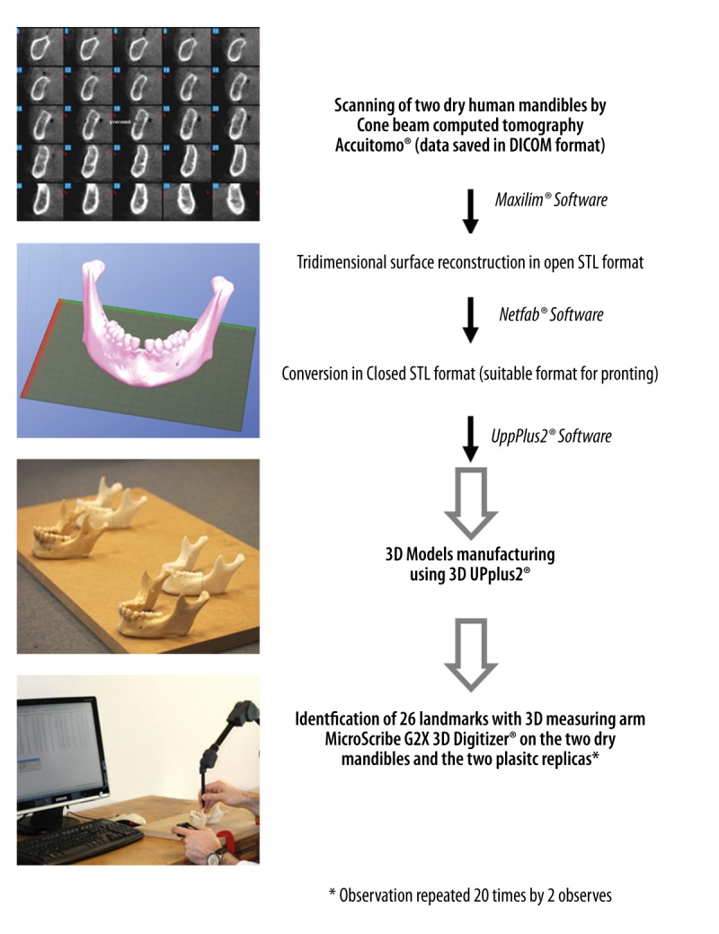
Sequence of methodological procedures.

Image preprocessing

Two dry human mandibles, named A and B, from the anatomical collection of Hasselt University, were scanned with a cone beam computed tomography (CBCT) device (Accuitomo^®, Morita, Kyoto, Japan). The radiological protocol was as follows: 90 kV, 5 mA, stereo mode, pixel size of 0.25 mm, slice thickness of 0.5 mm, and field of view of 140×100 mm. The scanning of dry mandibles was approved by the Ethics Committee of the University Hospitals of Leuven (authorization no. ML9593). The raw data were saved in DICOM format (Digital Imaging and Communications in Medicine). The 3D reconstruction of the 2 dry mandible surfaces was performed with Maxilim^® software (Medicim, Mechelen, Belgium), which also enables the conversion of the data to the STL format (Standard Template Library) and allows for a virtual model of surfaces consisting of a mesh of triangles. Then, Netfabb^® software version 4.9 (Netfabb GmbH, Lupburg, Germany) was used to repair the STL data and prepare it for use with the low-cost 3D printer UpPlus2^® software (Beijing TierTime Technology Co. Ltd., China).

3D model printing

The UPplus2^® 3D printer (Beijing TierTime Technology Co. Ltd., Beijing, China) is an RP machine based on a fused deposition modelling technique and uses ABS as a raw material. Three-dimensional models were created layer by layer with a 0.15-mm thickness, which is the minimal achievable thickness for that printer. The successive layers were composed of thermoplastic filament material that exited through a fine nozzle. The temperature of the printer nozzle for extruding ABS was 260–270°C. Three-dimensional printing is possible by the movement of the print-bed along the Z-axis associated with the movement of the print-head along the XY-axes. The printing of each model was performed in fine quality, which represents the most accurate printing option available for that printer. The model of mandible A was composed of 353 layers of 0.15 mm thickness (38.9 g of plastic), and 8 hours and 42 minutes were required to print the model in fine quality and with a lightweight filling modality. The model of mandible B was composed of 488 layers of 0.15 mm thickness (40 g of plastic), and the same time was required to print the model in fine quality and with a lightweight filling modality.

Measurements with 3D measuring arm

Two oral and maxillofacial surgeons with the same scientific background participated in this study as independent observers. A total of 26 anatomical landmarks were chosen for each mandible (Figure 2) to identify 13 anatomical distances. Each of the observers identified the osseous landmarks using the measuring arm MicroScribe G2X 3D Digitiser^® (Revware Systems Inc., USA). This arm possesses 6 degrees of freedom in 3D space and a precision of 0.30 mm. The identification of the 26 landmarks was performed by each observer on the surface of the 4 mandibles (2 dry mandibles and 2 replicas made of ABS) using the contact method of measuring. To decrease the potential error due to movements of the mandibles during the measurement process, the mandibles were fixed by means of metallic wires to a work plane, and the 3D measuring arm was fixed with clamps to the working plane. The 3D measuring arm and mandibles were positioned to obtain a 90° angle between the upper and the lower arm of the 3D measuring arm when the measurements were performed on 3D models, as is recommended by the manufacturer to achieve the optimal measurement accuracy. Moreover, the 3D measuring arm was provided with a self-calibration system that was used before each series of measurements. The system consisted of pressing a “home button” from a fixed point (“home position”) on the support of the 3D measuring arm. To decrease the involuntary movements of the observers, we used a joystick connected to the computer that provided a “copy and paste” option allowing immediate data collection on an Excel worksheet just by pressing a button.

Figure 2.

Landmark definitions. Mandible A (A) 1=Tooth#37: distal point, 2=Tooth#37: mesial point, 3=Tooth#36: distal point, 4=Tooth#36: mesial point, 5=Tooth#35: distal point, 6=Tooth#35: mesial point, 7=Tooth#32: distal point, 8=Tooth#32: mesial point, 9=Tooth#47: distal point, 10=Tooth#47: mesial point, 11=Tooth#46: distal point, 12=Tooth#46: mesial point, 13=Tooth#45: distal point; 14=Tooth#45: mesial point, 15=Tooth#42: distal point, 16=Tooth#42: mesial point, 17=Tooth#37: mesiolingual cusp, 18=Tooth#47: mesiolingual cusp, 19=Tooth#36: mesiolingual cusp, 20=Tooth#46: mesiolingual cusp, 21=Tooth#35: lingual cusp, 22=Tooth#45: lingual cusp, 23=Left lingual, 24=Right lingual, 25=Left coronoid, 26=Right coronoid. Mandible B (B) 1=Tooth#37: mesial point, 2=Tooth#37: distal point, 3=Tooth#36: distal point, 4=Tooth#36: mesial point; 5=Tooth#32: distal point, 6=Tooth#32: mesial point, 7=Tooth#31: distal point, 8=Tooth#31: mesial point, 9=Tooth#47: distal point, 10=Tooth#47: mesial point, 11=Tooth#46: distal point, 12=Tooth#46: mesial point, 13=Tooth#42: distal point, 14=Tooth#42: mesial point; 15=Tooth#41: distal point, 16=Tooth#4: mesial point, 17=Tooth#37: mesiolingual cusp; 18=Tooth#47: mesiolingual cusp, 19=Tooth#36: mesiolingual cusp, 20=Tooth#46: mesiolingual cusp, 21=Tooth#32: distal incisor angle, 22=Tooth#42: distal incisor angle, 23=Left Lingula, 24=Right Lingula, 25=Left coronoid, 26=Right coronoid.

To test intra- and inter-observer variability, 20 repeated measurements were recorded for each mandible and by 2 observers [4].

Microscribe Utility Software^® allowed each landmark to be located in the Cartesian coordinate system. Excel software was used to calculate the distances from the recorded coordinates (X, Y, Z) and enabled a comparison of the distances from dry mandibles measurements with those from plastic models. The distances were calculated using the formula below:

$$\text{Distance\hspace{0.17em}}1-2=\sqrt{{(X_{\mathit{1}}-X_{\mathit{2}})}^{\mathit{2}}+{(Y_{\mathit{1}}-Y_{\mathit{2}})}^{\mathit{2}}+{(Z_{\mathit{1}}-Z_{\mathit{2}})}^{\mathit{2}}}$$

Statistical analysis

The data were analyzed using descriptive statistics, and comparisons were performed with t tests for paired samples using SPSS software for Windows, version 16.0. According to the protocols of Choi et al. [3], Ibrahim et al. [4], and Silva et al. [7], we calculated the mean dimensional error (MDE) and mean absolute difference (MAD) for each linear distance using Excel software. The MAD was defined as the absolute difference (mm) between values obtained from the plastic replicas and the dry mandibles, as defined by the formula below:

$$\text{Absolute\hspace{0.17em}Difference}=Prototype\hspace{0.17em}Value-Dry\hspace{0.17em}Mandible\hspace{0.17em}Value$$

The MDE (%) was calculated as the absolute difference divided by the dry skull value ×100, as defined by the formula below:

$$\text{Mean\hspace{0.17em}Dimensional\hspace{0.17em}Error}=\text{Average\hspace{0.17em}}(\text{Mean\hspace{0.17em}Relative\hspace{0.17em}Difference})=\frac{Prototype\hspace{0.17em}Value-Dry\hspace{0.17em}Mandible\hspace{0.17em}Value}{Dry\hspace{0.17em}Mandible\hspace{0.17em}Value}\times \mathit{100}$$

To measure the inter- and intra-observer reproducibility, we performed a reliability analysis using SPSS software for Widows, version 16.0. Given that we used a fixed set of observers and population of observers (as opposed to a sample of observers), the analysis was performed using the 2-way mixed model based on absolute agreement for the group of measurements between the observer and type of material (mandible) [8,9].

Results

A larger number of observations obviously produces a superior platform for the statistical analysis of data and the identification of tangible patterns. While considering all the distances of the mandible to be similar, the entire data set of the observations was analyzed using paired t tests, and the values in Table 1 suggest that the data are statistically significant based on p-value of less than 0.05 (confidence interval of 95%).

Table 1.

Paired t test for the entire dataset of 13 distances of each mandible per observer.

Observer	Material	P Value	Statistically significant
1	A	0.045	Yes
1	B	0.000	Yes
2	A	0.032	Yes
2	B	0.000	Yes

Another approach to validate our analysis is to calculate the p-values for the observations of specific distances for each of the mandibles. The p-values are tabulated in Table 2. Paired t tests were performed for each of the distances, which resulted in 52 data sets, and the p-values for 80% of all data sets indicated statistical significance. Given the reasonably small number of observations for each of the data sets, and because approximately 62% of the datasets involved measurements less than 10 mm, we can infer that the overall data collection exercise and measurement techniques used are robust, with a negligible (very low) chance of a random error, which is a positive conclusion. The MAD and MDE values for each dataset are also provided in the tables for reference.

Table 2.

MAD (mm), MDE (%), P-value of the 13 distances.

Dry vs Plastic	MAD (mm)	MDE (%)	P-value
Mandible A – Observer 1
37 mesial-distal distance	0.088544423	1.035856057	0.048782295
36 mesial-distal distance	0.179550259	1.688349963	1.15257E-05
35 mesial-distal distance	0.103107493	1.560959009	0.005460712
32 mesial-distal distance	0.413485333	8.667998648	1.62667E-11
47 mesial-distal distance	−0.153230631	−1.708440182	0.001174151
46 mesial-distal distance	0.220184291	1.991622243	1.31471E-08
45 mesial-distal distance	−0.011072477	−0.12434094	0.769116977
42 mesial-distal distance	0.230619693	4.437794047	2.98411E-05
37ML37-47ML transversal distance	−0.054619646	−0.149171156	0.290251033
36ML36-46MLtransversal distance	0.132678587	0.437830862	0.01314919
35D-45D transversal distance	0.161291176	0.544774034	0.003426577
Left lingula-Right lingula transversal distance	0.230802644	0.321584293	4.32667E-05
Left coronoid-Right coronoid transversal distance	−0.942409206	−1.071435468	8.01392E-26
Total average	0.224738143	1.826165916
Mandible A – Observer 2
37 mesial-distal distance	−0.46310707	5.617506733	6.03759E-11
36 mesial-distal distance	0.104462422	−0.947094743	0.018191592
35 mesial-distal distance	−0.796754106	13.18756459	2.39918E-13
32 mesial-distal distance	−0.335507104	8.036458487	0.002715673
47 mesial-distal distance	−0.121180669	1.525808374	0.079627389
46 mesial-distal distance	0.053318111	−0.457813094	0.211062113
45 mesial-distal distance	−0.472058325	7.259261355	3.07802E-10
42 mesial-distal distance	−0.308208909	6.717292739	0.000518927
37ML37-47ML transversal distance	0.085807379	−0.231289614	0.344111282
36ML36-46MLtransversal distance	−0.51226346	1.711023727	2.77725E-06
35D-45D transversal distance	−0.300061336	1.019026177	0.260693121
Left lingula-Right lingula transversal distance	−0.785041711	1.090676192	0.31537105
Left coronoid-Right coronoid transversal distance	1.02554821	−1.163940712	1.75576E-12
Total average	0.412562986	3.766519734
Mandible B – Observer 1
37 mesial-distal distance	0.010497448	−0.072727022	0.804924784
36 mesial-distal distance	−0.047549022	0.404252321	0.043084928
32 mesial-distal distance	−0.500798967	9.480885407	1.60829E-13
31 mesial-distal distance	−0.354736665	6.831681084	1.782E-08
47 mesial-distal distance	−0.893234425	8.912647001	4.84733E-23
46 mesial-distal distance	0.544191829	−4.800088231	3.75898E-22
42 mesial-distal distance	−0.770122539	13.63726968	2.67664E-16
41 mesial-distal distance	−0.349362437	6.960800126	0.405030815
37ML37-47ML transversal distance	−0.280817054	0.723317659	2.60712E-06
36ML36-46MLtransversal distance	−0.328009609	0.997989394	2.91297E-08
32D-42D transversal distance	−0.332723444	1.326059812	7.73612E-08
Left lingula-Right lingula transversal distance	−0.32107201	0.423401457	1.79639E-09
Left coronoid-Right coronoid transversal distance	0.158228496	−0.17213352	0.00266376
Total average	0.376257227	4.21101944
Mandible B – Observer 2
37 mesial-distal distance	−0.162933121	1.522687392	0.207179604
36 mesial-distal distance	−0.808328805	11.09792384	0.251510188
32 mesial-distal distance	−0.873171721	18.38966191	2.34984E-09
31 mesial-distal distance	−0.392142608	8.460013379	0.001436505
47 mesial-distal distance	−0.785929443	7.99517563	4.97837E-14
46 mesial-distal distance	−0.01778071	0.170574757	0.739168776
42 mesial-distal distance	−0.623507819	11.9524075	6.99119E-09
41 mesial-distal distance	−0.053687496	1.406207697	0.657634945
37ML37-47ML transversal distance	−0.606414696	1.577931317	4.13583E-07
36ML36-46MLtransversal distance	−0.700146916	2.152745903	1.67848E-08
32D-42D transversal distance	−0.645382909	2.634619961	8.49803E-10
Left lingula-Right lingula transversal distance	−0.235399478	0.311644435	0.003052731
Left coronoid-Right coronoid transversal distance	0.592558138	−0.64153104	1.56204E-09
Total average	0.499798759	5.254855751

MAD – mean absolute difference; MDE – mean dimensional error.

Tables 3 and 4 list the intraclass correlation coefficient (ICC) values, which include single measurements as well as average measurements. Given that the data sets’ ICC values for the different materials are close to or equal to a value of 1, the results demonstrate an excellent degree of reproducibility and consistency for the ratings (measurements) obtained by the 2 observers.

Table 3.

ICC (intraclass correlation coefficient) values for Intra-observer reproducibility obtained from SPSS.

Intra-observer reproducibility (dry vs. plastic)
Observer 1 – Mandible A
Intraclass correlation		95% Confidence Interval
		Lower bound	Upper bound
Single measures	1.000	1.000	1.000
Average measures	1.000	1.000	1.000
Observer 1 – Mandible B
Intraclass correlation		95% Confidence Interval
		Lower bound	Upper bound
Single measures	1.000	1.000	1.000
Average measures	1.000	1.000	1.000
Observer 2 – Mandible A
Intraclass correlation		95% Confidence Interval
		Lower bound	Upper bound
Single measures	1.000	1.000	1.000
Average measures	1.000	1.000	1.000
Observer 2 – Mandible B
Intraclass correlation		95% Confidence Interval
		Lower bound	Upper bound
Single measures	1.000	1.000	1.000
Average measures	1.000	1.000	1.000

Table 4.

ICC (intraclass correlation coefficient) values for inter-observer reproducibility obtained from SPSS.

Inter-observer reproducibility
Mandible A – Material: Dry
Intraclass correlation		95% Confidence Interval
		Lower bound	Upper bound
Single measures	1.000	1.000	1.000
Average measures	1.000	1.000	1.000
Mandible A - Material: Plastic
Intraclass correlation		95% Confidence Interval
		Lower bound	Upper bound
Single measures	0.994	0.993	0.995
Average measures	0.997	0.996	0.998
Mandible B – Material: Dry
Intraclass correlation		95% Confidence Interval
		Lower bound	Upper bound
Single measures	0.999	0.999	1.000
Average measures	1.000	1.000	1.000
Mandible B – Material: Plastic
Intraclass correlation		95% Confidence Interval
		Lower bound	Upper bound
Single measures	1.000	1.000	1.000
Average measures	1.000	1.000	1.000

In our study, the MDE value was 3.76% because 8 of the 13 measured distances were smaller (less than 12 mm) than those of all other studies, which utilized linear distances that were 2 to 10 times longer (Table 5). Our findings were similar to those of Barker et al., who found that a higher MDE was associated with distances smaller than 25 mm [10]. A gross visual examination indicated that dental landmarks, such as the incisor angles (Figure 3), the cusps (Figure 4), and the interproximal dental contacts (Figure 5), exhibited different shapes in dry and plastic mandibles. This fact could also explain a more important MDE value that was calculated from short distances and based on dental landmarks. The MDE value decreased to 0.77% for mandible A and to 1.09% for mandible B when considering only the 5 transverse distances larger than 12 mm (Table 6). We can also note that observer no. 2 was less rigorous in using 3D measuring arm MicroScribe than the observer no. 1 (Table 6). In previous studies [3–5,7] only 1 observer performed measurements that were repeated 20 times. Our study shows that inter-observer variability may exist when working with a 3D measuring arm.

Table 5.

Comparison of material, methodology, and results of the present study (new low-cost 3D printer) and similar studies (standard high-cost 3D printing technologies) reported in the literature.

Author	RP technology, name 3D printer	Comparison	Radiological protocol	Software used	Measuring protocol (observers, landmark, distances)	Type of measuring device	MAD (mm)	MDE (%)
Barker et al. (1994) [10]	SL, SLA-250 (3D Systems Inc., CA, USA)	SL-1 dry skull	GE 9800 (GE Medical Systems, WI, USA) 70 mA, 120 kV, 1.5 mm slice thickness, interval of 1.5 mm, Table feed 1.5 mm	Analyze 5.0 (Biotechnology Computer Resource, Mayo Foundation, MN, USA) for bone segmentation and 3D reconstruction	19 landmarks (definitions not provided), 11 distances 1 observer, 5 times	Vernier calliper with dial gauge display (resolution ± 0.05 mm)	+0.85 mm (+4.62 mm maximum) to +0.1 mm (minimum)	Minimum of 0.6% to maximum of 3.6%
Ono et al. (1994) [13]	SL, SCS-1000 HD (Sony, Japan), layer thickness of 0.20 mm	CT-1 dry skull SL-1 dry skull	3D CT TCT-900S (Toshiba, Tokyo, Japan)	Not provided	10 distances (landmarks definitions not provided)	Not provided	Not provided	<3%
Kragskov et al. (1996) [14]	SL, SLA 250 (3-D-Systems, Valencia, CA, USA), layer thickness of 0.25 mm	3-D CT model-RP model (5 models)	Somatom DRH, Somatom plus (Siemens, Erlangen, Germany) 280 mA, 125 kV, 2mm section thickness, matrix size 512×512	Mimics, (Materialise, Leuven, Belgium) for bone segmentation Camra (ISG, Toronto, Canada) for 3D reconstruction	10 landmarks (definitions provided), 15 distances, comparison between measurements on 2D cephalograms and 3D SL model	Calliper	1.98 mm (minimum of −1.80 mm to 5.84 mm)	3.59% (minimum of −1.85% to maximum of 11.33%)
Berry et al. (1997) [15]	SLS (Sinterstation 2000) layer thickness of 0.1 mm	SLS-3D CT, 2 skulls	Siemens Somatom Plus SCT, 1 mm slice thickness	Analyze 7.0 (image segmentation)	Landmarks definitions not provided, 3 distances	Not provided	1.0 mm	0.64%
Bouyssié et al. (1997) [16]	SL, SLA 250 (3D-Systems, Valencia, USA), layer thickness of 0.125 mm, Somos epoxy resin	SL-2 dry mandibles	Elscint 2400 Elite CT scan, matrix size 512×512, 120 kv, 200 mAs, 1 mm interval, 1.2 mm slice thickness	Mimics (Materialize, Leuven, Belgium) bone segmentation at 1400 HU and 1254 HU CT-modeler software for interplane linear interpolation	9 landmarks, (definitions not provided), 12 linear distances, 3 observers (measured once)	Calliper	0.12 mm	Mean dimensional accuracy of 97.9%
Asaumi et al. (2001) [17]	SL (Desolite SCR 301, Japan Gum Co., Tokyo, Japan)	3D CT-1 dry mandible 1 SL-1 dry mandible	3DCT 900S scanner (Toshiba, Tokyo, Japan), 120 kV, 100 mA. 1 mm slice thickness, and 1 mm spacing, bone threshold value 200 HU	Not provided	27 landmarks, (definitions not provided), 17 measurement, 2 observers, repeated measurements after 1 week	Calliper for dry skull on 3D CT monitor for 3D imaging	Not provided	2.16 (−17.2% for alveolar width in the maxilla to 4.7% for upper facial width) 0.63% (−1.5% middle facial width to 1.1% between prosthion and basion)
Choi et al. (2002) [3]	SL (SLA 5000, 3D Systems, Valencia, CA, USA),	3D CT-1 dry skull and 1 mandible SL-1 dry skull and 1 mandible SL-3D CT	Somatom Plus 4 (Siemens, Erlangen, Germany) 1.5 mm section interval, 1 mm slice thickness, 512×512 matrix, pitch of 1.5, 200 mA, 120 KVP	V-works (CyberMed Inc., Seoul, Korea) for STL transformation	12 landmarks, (definitions provided), 16 distances, 1 observer, 20 times	Callipers (Mitutoyo, Japan) for dry skull Magicsview software (Materialise, Harislee, Belgium) for 3D imaging	0.49 mm (SD: 0.34) 0.62 mm (SD: 0.35) (minimum of −1.22 mm to maximum of +1.06 mm) 0.57 mm (SD: 0.62)	0.65% 0.56% (minimum of −1.89% to maximum of +0.86%) 0.82%
Chang et al. (2003) [18]	SL, (Z402 3-D Printer, Z Corporation, Burlington, MA)	SL-cadaver skulls (9 fresh cadavers)	CT (Highlight Advantage Scanner; GE Medical Systems, Waukesha, WI), slice spacing of 1.5 mm, field of view of 25 cm, with pixel resolution of 0.49 mm per pixel	Mimics and CTM software (Materialise USA, Ann Arbor, MI) for bone segmentation, 3D reconstruction, and STL transformation	19 osseous landmarks (definitions provided), 70 linear measurements per skull, 1 observer, measurements performed once on fresh skulls and corresponding SL replica	Precision (100-μm resolution) dial callipers (Mitutoyo America Corporation, Aurora, IL)	1.5 mm (range: 0–5.5 mm) for craniofacial measures, 1.2 mm (range: 0–4.8 mm) for skull base measures, 1.6 mm (range: 0–5.8 mm) for midface measures, 1.9 mm (range: 0–7.9 mm) for maxilla measures, 1.5 mm (range: 0–5.7 mm) for orbital measures	2.1% 2.0% 4.0% 4.3% 4.7%
Nizam et al. (2006) [19]	SL, (SLA Viper Si2, 3D Systems, Valencia, CA, USA).	SL-dry skulls (4 skulls)	Light Speed Plus (General Electric Medical System, U.S.A.), 1.25 mm Slice thickness in spiral mode and a 512 × 512 Matrix, a pitch of 1.5, 200 mA, 120 KVp	Mimics (Materialise, Leuven, Belgium) for bone segmentation	9 landmarks (definitions provided), 8 distances, 1 observer, repeats 5 times each measurement	Electronic digital calliper (Ultra Gold Pro-Max, Fowler-NSK, Japan)	0.23±1.37 mm	0.08±1.25%
Silva et al. (2008) [7]	SLS, Sinteristation 2000 (DTM, USA), thin polyamide powder (PA 2200, EOS, Munich, Germany), finishing with sandblasting 3DP, ZPrinter 310 System (MIT, MA, USA), plaster powder (zp102, Z Corporation, Burlington, USA) and a water-based binder. Finishing with application of a cyanoacrylate-based infiltration material (Z-Bond100, Z Corporation, Burlington, USA)	SLS-1 dry skull 3DP-1 dry skull	helical CT unit (Somatom Plus 4, Siemens, Munich, Germany) with 0_ gantry tilt; 1 mm slice thickness; 1.5 pitch; field of view (FOV) 20.8 cm; matrix 512×512; 120 kVp; and 130 mA	InVesalius software (CenPRA, Campinas, Brazil) to bone segmentation at 400–3300 HU threshold	14 landmarks (definitions provided), 10 distances, 1 observer, each measurement repeated 20 times by one observer	Starrett electronic calliper (Starrett Ind. e Com. Ltda, Sao Paulo, Brazil)	0.89 mm 1.07 mm	2.10% 2.67%
Ibrahim et al. (2009) [4]	SLS, Sinterstation 2000 3DP, ZPrinter 310 System Polyjet, EDEN 330 (ARTIS, Brasilia-DF, Brasilia)	SLS-1 dry mandible 3DP-dry mandible Polyjet-dry mandible	Not provided	InVesalius software STL model with 583468 triangles	8 anatomical landmarks (definitions provided), 13 linear measurement, each measurement repeated 20 times by one observer	Digital electronic calliper	0.90 mm 1.44 mm 1.23 mm	1.79% 3.14% 2.14%
El-Katatny et al. (2010) [20]	FDM, FDM 3000 (Stratasys), ABS plastic material and soluble support material, slice height 0.25 mm, finishing with support removal, cleaning and polishing	FDM-3D CT, 3 skulls FDM-3D CT, 3 mandibles	Not described	InVesalius software (2008), bone segmentation with threshold values of 1200 to 4000 Magics software for 3D reconstruction and STL repair	8 landmarks (definitions provided), 20 linear distances, measurements repeated 5 times	NSK MAX-Series Electronic Digital calliper Magics software for 3D measurements on screen	0.1mm (minimum 0.02 mm, maximum 0.25 mm) for skull 0.079 mm (minimum of 0.035mm and maximum of 0.2 mm) for mandible	0.24% 0.22%
Salmi et al. (2013) [12]	SLS (EOSINT P380 & SLS2200 (EOS GmbH, Munich, Germany), slice thickness 0.15mm 3DP, Zprinter 450 & ZP 150 (Z Corporation Burlington, USA), slice thickness 0.09mm Polyjet, Objet Eden 350 V & VeroWhite FullCure 830 (Objet Ltd, Rehovot, Israel), slice thickness 0.016mm	SLS-3D CT, (2 skull models) 3DP-3D CT (4 skull models) Polyjet-3D CT (2 skull models)	OsiriX DICOM sample image set CT machine and radiological protocol not provided)	OsiriX 2.7.5 (open source) software, bone segmentation at 500 HU STL model modification (original, moderate, worse models) with Viscamp RP 4.0 software (Marcam Engineering GmbH, Bremen, Germany)	6 measuring balls placed on virtual 3D CT model, 15 distances, contact with balls repeated automatically 12 times	3D coordinate measuring machine (CMM) ZEISS C 700 (Carl Zeiss AG, Oberkochen, Germany) with measuring tip of 4mm diameter (RENISHAW PH 1 (Renishaw Plc, New Mills, United Kingdom), measuring force was 68.7 mN Pro Engineer software for 3D CT models measurements	Not provided	0.79±0.26% (1st model), and 0.80±0.32% (2nd model) 0.67±0.43% (original model’s first measurement), 0.69±0.44% (original model’s second measurement), 0.38±0.22% (moderate model), and 0.55±0.37% (worse model) 0.18±0.12% (first measurement), and 0.18±0.13% (second measurement)
Present study (2015)	FDM low-cost (Up2 plus), plastic ABS, thickness of 0.1	FDM-dry mandible (2 mandibles)	CBCT (Accuitomo, Morita, Japan), with 90 kV, 5 mA, stereo mode; pixel size of 0.25 mm, 0.5 mm slice thickness, and field of view of 140×100	Maxilim (Medicim, Mechelen, Belgium) for bone segmentation, 3D reconstruction Netfabb Professional for STL repair Up2 plus software for 3D printing	26 landmarks (definition provided) 2 observers, each observer repeated 20 times the measurements	3D measuring arm (MicroScribe G2X 3D Digitizer® (Revware Systems Inc, USA)	For all distances: 0.37 mm For distances >12 mm: 0.42 mm	For all distances: 3.76% For distances >12 mm: 0.93%

MAD – mean absolute difference, MDE – mean dimensional error.

Figure 3.

Comparison between dry (A) and plastic mandible (B): Example of incisor angle and inter-dental distance.

Figure 4.

Comparison between dry (A) and plastic mandible (B): Example of molar cusps.

Figure 5.

Comparison between dry (A) and plastic mandible (B): Measuring tip positioning on interproximal dental contacts.

Table 6.

MDE (%) and MAD (mm) of the distances larger than 12 mm (transverse distances).

	MAD (mm)		MDE (%)
	Mandible A	Mandible B	Mandible A	Mandible B
Observer 1	0.3043	0.2841	0.5049	0.7285
Observer 2	0.5417	0.5559	1.0431	1.4636
Average	0.423	0.42	0.774	1.09

MAD – mean absolute difference, MDE – mean dimensional error.

Discussion

Three-dimensional RP replicas are used for almost every indication in craniomaxillofacial surgery [2,6]. The accuracy of 3D RP medical models has already been extensively tested for the main types of RP professional high-cost technologies, such as SL, SLS, 3DP, and FDM printing technologies (Table 5). The accuracy testing for low-cost 3D printers was initiated by Olszewski et al. [11] in 2014 with experimental validation of models from paper-based 3D printer (Mcor Technologies, Eire), and by Petropolis et al. in 2015 with low-cost FDM printer using PLA filament.

With the use of the Up plus 2 printer we found a similar range of values for MDE as Petropolis et al. [5]. However we found that modifications of MDE may be related to the: 1) range of chosen distances (more or less than 12 mm), 2) choice of landmarks on different types of anatomic areas (bone versus teeth areas); and 3) the individual anatomy of the bony piece to be replicated (difference of MDE between mandible A and B). We were also able to provide intra- and interobserver reproducibility, which was not performed in the Petropolis study [5].

Moreover, no methodological gold standard currently exists to validate the accuracy of 3D models from professional RP printers (Table 5) [12,13]. We found a great variability in methodological approaches when testing the accuracy of different types of 3D RP systems (Table 5). Diverse types of comparison were performed: 3D model versus dry skull/fresh cadaver, dry skull versus image modality (virtual 3D reconstruction), image modality (virtual 3D reconstruction) versus 3D model (Table 5). Different radiological protocols with various threshold values for bone segmentation were used. Multiple software were used for preprocessing the data and generating the final printable STL file. Numerous protocols/parameters were used to manufacture 3D RP models (type of raw material, slice thickness). Different post-processing and finishing steps were necessary to obtain a final model. Various types of accuracy measurements were performed with differences in the: 1) number of landmarks, 2) type of landmarks, 3) type of linear distances, 4) number of observers, 5) number of repetition of measurements, 6) type of measuring instrument used and its resolution (Table 5) [3,4,7,10,12,14–20].

Low-cost 3D printers represent a great opportunity in the medical field, as they could allow surgeons to use 3D models at a very low cost and, therefore, democratize the use of these 3D models in all previously described and new indications. However, efforts should be made to establish a unified validation protocol (which should be part of an international consensus) for low-cost RP 3D printed models, including accuracy, reproducibility, and repeatability tests (and reporting technical information in the same style). Asaumi et al. suggested that dimensional changes may not affect the success of surgical applications if such changes are within a 2% variation [17]. However, the proposed cut-off of 2% should be discussed, as the same accuracy may be not required for all types of indications [7]. Moreover, 3D RP low-cost models must also be clinically optimized, as models used in in vitro studies were done with the best-performing parameters for 3D printers. The use of different slice thicknesses, printing speeds, support table heating times, and methods of filling empty spaces should also be investigated and adapted for each specific indication.

The accuracy of a printed 3D model also greatly depends on the accuracy of the initial virtual model (Maxilim) [2]. Therefore, a further study should compare the virtual model of the mandible and teeth with the 3D CT or CBCT scan of the same 3D printed mandible. Such a study may explain why differences occur at the level of fine structures (on the teeth) when we compare the dry mandible to 3D printed models (Figures 3–5).

Another aspect that should also be investigated is possible methods to sterilize 3D RP FDM ABS models to allow their further use in the operating room without any harm to the patient. Additionally, the cytotoxicity of the raw material (ABS), which is provided by companies, must be tested. If 3D RP FDM models are to serve only as a preoperative diagnostic anatomical model or may serve to prebend plates, we need to determine only the accuracy of the specific 3D low-cost printer. However, when a 3D model is intended to be used in the operating room (for example, as a cutting guide) then accuracy, sterilization, and cytotoxicity tests are indispensable steps to convince any ethics committee of the safety of the product to be used.

Conclusions

Finally, our hypothesis that the accuracy of the 3D plastic replicas generated with a low-cost 3D FDM printer would be clinically acceptable appears to be correct for distances greater than 12 mm. Plastic ABS models printed by the low-cost 3D printer UPplus2^® provide dimensional accuracy comparable to other well-established high-cost professional RP technologies. We did not find any warping on printed and measured ABS models from the Up plus 2 3D FDM printer. Validated low-cost FDM printers could represent a next step toward better accessibility of RP technologies and their use in-house for most surgeons.

References

- 1.Mankovich NJ, Cheeseman AM, Stoker NG. The display of three-dimensional anatomy with stereolithographic models. J Digit Imaging. 1990;3:200–3. doi: 10.1007/BF03167610. [DOI] [PubMed] [Google Scholar]
- 2.Winder J, Bibb R. Medical rapid prototyping technologies: state of the art and current limitations for application in oral and maxillofacial surgery. J Oral Maxillofac Surg. 2005;63:1006–15. doi: 10.1016/j.joms.2005.03.016. [DOI] [PubMed] [Google Scholar]
- 3.Choi JY, Choi JH, Kim NK, et al. Analysis of errors in medical rapid prototyping models. Int J Oral Maxillofac Surg. 2002;31:23–32. doi: 10.1054/ijom.2000.0135. [DOI] [PubMed] [Google Scholar]
- 4.Ibrahim D, Broilo TL, Heitz C, et al. Dimensional error of selective laser sintering, three-dimensional printing and PolyJet models in the reproduction of mandibular anatomy. J Craniomaxillofac Surg. 2009;37:167–73. doi: 10.1016/j.jcms.2008.10.008. [DOI] [PubMed] [Google Scholar]
- 5.Petropolis C, Kozan D, Sigurdson L. Accuracy of medical models made by consumer-grade fused deposition modeling printers. Plast Surg (Oakv) 2015;23:91–94. doi: 10.4172/plastic-surgery.1000912. [DOI] [PMC free article] [PubMed] [Google Scholar]
- 6.Ernoult C, Bouletreau P, Meyer C, et al. Reconstruction assisted by 3D printing in maxillofacial surgery. Rev Stomatol Chir Maxillofac Chir Orale. 2015;116:95–102. doi: 10.1016/j.revsto.2015.01.010. [DOI] [PubMed] [Google Scholar]
- 7.Silva DN, Gerhardt de Oliveira M, Meurer E, et al. Dimensional error in selective laser sintering and 3D-printing of models for craniomaxillary anatomy reconstruction. J Craniomaxillofac Surg. 2008;36:443–49. doi: 10.1016/j.jcms.2008.04.003. [DOI] [PubMed] [Google Scholar]
- 8.Shrout PE, Fleiss JL. Intraclass correlations: uses in assessing rater reliability. Psychological Bulletin. 1979;86:420–42. doi: 10.1037//0033-2909.86.2.420. [DOI] [PubMed] [Google Scholar]
- 9.McGraw KO, Wong SP. Forming inferences about some intraclass correlation coefficients. Psychological Methods. 1996;1:30–46. [Google Scholar]
- 10.Barker TM, Earwaker WJS, Lisle DA. Accuracy of stereolithographic models of human anatomy. Australasian Radiology. 1994;38:106–11. doi: 10.1111/j.1440-1673.1994.tb00146.x. [DOI] [PubMed] [Google Scholar]
- 11.Olszewski R, Szymor P, Kozakiewicz M. Accuracy of three-dimensional, paper-based models generated using a low-cost, three-dimensional printer. J Craniomaxillofac Surg. 2014;42:1847–52. doi: 10.1016/j.jcms.2014.07.002. [DOI] [PubMed] [Google Scholar]
- 12.Salmi M, Paloheimo KS, Tuomi J, et al. Accuracy of medical models made by additive manufacturing (rapid manufacturing) J Craniomaxillofac Surg. 2013;41:603–9. doi: 10.1016/j.jcms.2012.11.041. [DOI] [PubMed] [Google Scholar]
- 13.Ono I, Gunji H, Suda K, Kaneko F. Method for preparing an exact-size model using helical volume scan computed tomography. Plast Reconstr Surg. 1994;93:1363–71. doi: 10.1097/00006534-199406000-00005. [DOI] [PubMed] [Google Scholar]
- 14.Kragskov J, Sindet-Pedersen S, Gyldensted C, Jensen KL. A comparison of three-dimensional computed tomography scans ad stereolithographic models for evaluation of craniofacial anomalies. J Oral Maxillofac Surg. 1996;54:402–11. doi: 10.1016/s0278-2391(96)90109-3. [DOI] [PubMed] [Google Scholar]
- 15.Berry E, Brown JM, Connell M, et al. Preliminary experience with medical applications of rapid prototyping by selective laser sintering. Med Eng Phys. 1997;19:90–96. doi: 10.1016/s1350-4533(96)00039-2. [DOI] [PubMed] [Google Scholar]
- 16.Bouyssié JF, Bouyssié S, Sharrock P, Duran D. Stereolithographic models derived from x-ray computed tomography. Reproduction accuracy. Surg Radiol Anat. 1997;19:193–99. [PubMed] [Google Scholar]
- 17.Asaumi J, Kawai N, Honda Y, et al. Comparison of three-dimensional computed tomography with rapid prototype models in the management of coronoid hyperplasia. Dentomaxillofac Radiol. 2001;30:330–35. doi: 10.1038/sj/dmfr/4600646. [DOI] [PubMed] [Google Scholar]
- 18.Chang PS, Parker TH, Patrick CW, Jr, Miller MJ. The accuracy of stereolithography in planning craniofacial bone replacement. J Craniofac Surg. 2003;14:164–70. doi: 10.1097/00001665-200303000-00006. [DOI] [PubMed] [Google Scholar]
- 19.Nizam A, Gopal RN, Naing L, et al. Dimensional accuracy of the skull models produced by rapid prototyping technology using stereolithography apparatus. Arch Orofac Sci. 2006;1:60–66. [Google Scholar]
- 20.El-Katatny I, Masood SH, Morsi YS. Error analysis of FDM fabricated medical replicas. Rapid Prototyping J. 2010;16:36–43. [Google Scholar]