Binomial mixture model-based association testing to account for genetic heterogeneity for GWAS

Abstract

Genome-wide association studies (GWASs) have confirmed the ubiquitous existence of genetic heterogeneity for common disease: multiple common genetic variants have been identified to be associated, while many more are yet expected to be uncovered. On the other hand, the single SNP-based trend test (or its variants) that has been dominantly used in GWASs is based on contrasting the allele frequency difference between the case and control groups, completely ignoring possible genetic heterogeneity. In spite of the widely accepted notion of genetic heterogeneity, we are not aware of any previous attempt to apply genetic heterogeneity-motivated methods in GWAS. Here, to explicitly account for unknown genetic heterogeneity, we applied a mixture model-based single SNP test to the WTCCC GWAS data with traits Crohn’s disease, bipolar disease, coronary artery disease and type 2 diabetes, identifying much larger numbers of significant SNPs and risk loci for each trait than those of the popular trend test, demonstrating potential power gain of the mixture model-based test.

1 Introduction

Genome-wide association studies (GWASs) have been extremely successful in identifying thousands of common genetic variants, mostly single nucleotide polymorphisms (SNPs), associated with common disease and complex traits (NHGRI Catalog: http://wwww.genome.gov/gwastudies/). Some important discoveries on the genetic architecture for complex traits are the following. First, genetic heterogeneity is everywhere: multiple SNPs and risk loci have been identified for many common disease and complex traits, suggesting the plausibility and even ubiquity of a polygenic model. Second, the effect sizes of most causal SNPs are estimated to be from moderate to small, many of which with smaller effect sizes are yet to be identified. Consequently, larger sample sizes and more powerful statistical tests are always needed in order to identify more risk loci. On the other hand, almost all GWASs have adopted single SNP-based analysis without explicitly accounting for (unknown) genetic heterogeneity, leading to possible loss of power as convincingly shown in simulation studies (Zhou and Pan 2009; Londono et al 2012; Qian and Shao 2013). Note here we consider unknown genetic heterogeneity here, rather than known phenotype heterogeneity as discussed in Darabi and Humphreys (2011). Based on a two-component binomial mixture model of Zhou and Pan (2009), if any given locus contains a causal SNP, then the patient population is decomposed into two subpopulations: the first subpopulation consists of the patients whose disease is associated with the disease allele at the locus, while the second includes those with disease caused by other unknown alleles at other unknown risk loci. In addition to contrasting the allele frequencies (i.e. means or first moments) between the control and case groups as targeted by the most popular 1df trend test, the proposed mixture model can capture some other distributional differences of the allele (i.e. second moments) between the two groups. For example, in an extreme case, even if there is barely any difference of the allele frequencies between the two groups, leading to no power of the trend test, if the mixture model assumption holds, then a mixture model-based likelihood ratio test (LRT-H) may still be able to detect the distributional differences of the allele between the two groups. Qian and Shao (2013) extended the two-component binomial mixture model to one with more than two components, for which an LRT-H statistic with a simple closed-form and an asymptotic null distribution was derived, facilitating its application to GWAS. Surprisingly, to our knowledge, it has not yet been applied to any GWAS. In fact, we are not aware of any other analyses of GWASs that explicitly account for genetic heterogeneity. Here we review the LRT-H and apply it to the WTCCC GWAS data. To ensure that our conclusion is not limited to any specific disease, we considered multiple diseases. We demonstrate that the LRT-H test can be much more powerful than the popular trend test in identifying a much larger number of associated SNPs and risk loci.

2 Methods

For each subject i, suppose X_i = 0, 1 or 2 is the number of the minor allele of a SNP to be tested, and Y_i = 0 or 1 is the disease indicator. The methods are all based on single SNP analysis by testing on each SNP individually and separately, hence we can focus on only one SNP. The goal is to test for possible association between the SNP and disease.

The trend test and related tests

Most of the existing association tests ignore possible genetic heterogeneity due to the disease. For example, the most popular Cochran-Armitage 1df trend test can be formulated as the Score test in a logistic regression model (Wellek and Ziegler 2011) (or more generally a GLM or Cox PHM for other types of traits)

$$\text{logit}(Pr(Y_i=1))={\beta }_0+{\beta }_1{X}_i$$ (1)

to test the null hypothesis H₀: β₁ = 0. It is well known (Clayton et al 2004) that the Score test is

$$T_S=\frac{{\overline{X}}^{(1)}-{\overline{X}}^{(2)}}{\sqrt{\widehat{\text{Var}}({\overline{X}}^{(1)}-{\overline{X}}^{(2)})}},$$

where X̄^(d) is the sample mean of X_i’s with Y_i = d for d = 0 or 1. The Score test is asymptotically equivalent to the Z-test for one SNP (and equivalent to Hotelling’s T² test for multiple SNPs (Xiong et al 2002; Fan and Knapp 2003)). Specifically, one can model the conditional distribution of X_i as binomial:

$$X_i\mid Y_i=0~\mathit{Bin}(2,{\theta }_0),X_i\mid Y_i=1~\mathit{Bin}(2,{\theta }^{\ast }),$$

for which we’d like to test the null hypothesis $H_0^{\prime }:{\theta }_0={\theta }^{\ast }$, which is equivalent to the original H₀. It is easy to see that, the Wald test for $H_0^{\prime }$ is

$$T_W=\frac{{\overline{X}}^{(1)}-{\overline{X}}^{(2)}}{\sqrt{\stackrel{\sim }{\text{Var}}({\overline{X}}^{(1)}-{\overline{X}}^{(2)})}},$$

which differs from T_S in the variance estimates used in the denominator, but nonetheless is asymptotically equivalent to T_S. Furthermore, the asymptotically equivalent likelihood ratio test (LRT) can be also applied:

$$T_L=2log(L_H{L}_D)-2log{L}_0$$

with

$$L_H=\prod _{g=0}^2{B}_2{(g,{\widehat{\theta }}_0)}^{m_g},L_D=\prod _{g=0}^2{B}_2{(g,{\widehat{\theta }}_1)}^{n_g},L_0=\prod _{g=0}^2{B}_2{(g,{\widehat{\theta }}_{01})}^{m_g+n_g},$$

where n_g and m_g are the genotype frequencies as summarized in Table 1, the maximum likelihood estimates (MLEs) of the minor allele frequencies (MAFs) under H₀ and H₁ are

Table 1.

The genotype frequencies for case-control data of a SNP.

	AA	Aa	aa	Total
Case	n0	n1	n2	n
Control	m0	m1	m2	m

$${\widehat{\theta }}_{01}=\frac{2n_2+2m_2+n_1+m_1}{2n+2m},{\widehat{\theta }}_0=\frac{2m_2+m_1}{2m},{\widehat{\theta }}_1=\frac{2n_2+n_1}{2n},$$

and

$$B_2(g,p)=Pr(X=g)=\left(\begin{array}{c}2\\ g\end{array}\right)p^g{(1-p)}^{2-g}$$

is the probability mass function for a binomial distribution X ~ Bin(2, p).

The above three tests all share the same (asymptotic) null distribution as a chi-squared distribution ${\chi }_1^2$ with 1 df.

Rather than using a trend test based on the additive genetic model for X_i, a more general 2df test can be formulated by fitting an expanded regression model:

$$\text{logit}(Pr(Y_i=1))={\beta }_0+{\beta }_1{X}_i+{\beta }_2{X}_i^2,$$ (2)

and we test $H_0^{″}:{\beta }_1={\beta }_2=0$ with one of the three asymptotically equivalent Score test, Wald test and LRT, all with an asymptotically null distribution of ${\chi }_2^2$ with df=2. Interestingly, as pointed out by Kim et al (2010), β₂ measures the difference of Hardy-Weinberg coefficients in the disease and control groups, hence a 2df test can be regarded as testing on both allele frequency difference and Hardy-Weinberg coefficient difference between the two groups. In this paper, we used R function glm() to fit a logistic regression model and applied the Wald test.

Hardy-Weinberg Equilibrium (HWE) exact test

A Hardy-Weinberg Equilibrium (HWE) test can be applied to the case group (with notation shown in Table 1) for association analysis (Nielsen et al 1998). Given that the total number of observed minor allele is n_a = 2n₂ + n₁, under the assumption of HWE, the probability of observing n₁ heterozygotes:

$$P(N_1=n_1\mid n,n_a)=\frac{2^{n_1}n!}{n_2!n_1!n_0!}\times \frac{n_a!(2n-n_a)!}{(2n)!},$$ (3)

and the p-value is calculated as

$$P_{\mathit{HWE}}=\sum _{n_1^{\ast }}I[P(N_1=n_1\mid n,n_a)\ge P(N_1=n_1^{\ast }\mid n,n_a)]\times P(N_1=n_1^{\ast }\mid n,n_a).$$ (4)

We conducted the HWE exact test of Wigginton et al (2005) as implemented in function hwexact() from R package hwde.

Association testing under genetic heterogeneity

To fully and explicitly account for genetic heterogeneity, Zhou and Pan (2009) proposed a binomial mixture model for the disease group while using a usual binomial model for the control group:

$$X_i\mid Y_i=0~\mathit{Bin}(2,{\theta }_0),X_i\mid Y_i=1~\pi \mathit{Bin}(2,\theta )+(1-\pi )\mathit{Bin}(2,{\theta }_0),$$ (5)

where θ₀ is the background MAF for the controls. In contrast, for the case group, we assume θ is the probability of having the minor allele on a chromosome for a subpopulation of cases with disease caused by (or associated with) the minor allele, while for other subpopulations of cases the disease is caused by (unknown) variants at other unlinked loci, and thus for them the probability of having the minor allele at the locus of interest is the same as that for the controls. We test H₀ : θ = θ₀ or π = 0. Zhou and Pan (2009) considered more general scenarios with different θ₀’s for cases and controls, or with more than one non-null component for cases, but recommended the above two-component mixture model due to the non-identifiability issues with the more general models.

There are several important implications from the mixture model. First, the mixture model differs from the usual (implicit) assumption of $X_i^{\ast }\mid Y_i=1~\mathit{Bin}(2,{\theta }^{\ast })$ with θ^* = πθ + (1 − π)θ₀ for cases. Although E(X) = E(X^*), it is shown (Zhou and Pan 2009) that

$$E(X_i^2\mid Y_i=1)-E(X_i^{\ast 2}\mid Y_i=1)=\pi (1-\pi ){(\theta -{\theta }_0)}^2\ge 0,$$

where the strict inequality holds for the non-degenerated case with θ^* ≠ θ₀, π ≠ 0 and π ≠ 1. Hence, the binomial mixture model introduces an overdispersion of the minor allele as compared to a binomial distribution with the same MAF. While the most popular 1df trend test compares the mean difference of the genotype scores between the control and case groups, it ignores the possible genetic heterogeneity in the case group and thus possible differences in high moments of the genotype scores between the two groups. Hence, taking advantage of the existing genetic heterogeneity (as modeled by the mixture model), an association test can gain power in detecting differences in both the means (i.e. first moments) and higher-order moments (e.g. second moments) between the control and case groups, which is closely related to the expanded regression model (2). Second, as shown by Zhou and Pan (2010), the mixture model also implies that HWE is violated in the case group under genetic heterogeneity, suggesting its connection to the HWE test.

Since complex diseases can be caused by a large number of genetic variants, it may be desirable to use a mixture model with more than two components to capture the complex heterogeneity. Qian and Shao (2013) extended the two-component mixture model to a more general form for the disease group as follows:

$$X_i\mid Y_i=1~\sum _{j=1}^J{\pi }_j\mathit{Bin}(2,{\theta }_j),$$ (6)

with J ≥ 2, 0 < θ_j < 1 and π_j ≥ 0 for any j = 1, …, J, and ${\sum }_{j=1}^J{\pi }_j=1$. Note that J ≥ 2 is unknown and does not need to be specified.

To test the null hypothesis H₀: θ₁ = θ₂ = ··· = θ_J (or π_j = 1 and π_k = 0 ∀k ≠ j), Qian and Shao (2013) developed a likelihood ratio test under genetic heterogeneity (LRT-H). The likelihoods L_H and L₀ are the same as before except

$$L_D=\{\begin{array}{ll}{\prod }_{g=0}^2{B}_2{(g,{\widehat{\theta }}_1)}^{n_g},\hfill & \text{if}4n_0{n}_2\le n_1^2;\hfill \\ {\prod }_{g=0}^2{(n_g/n)}^{n_g},\hfill & \text{if}4n_0{n}_2>n_1^2.\hfill \end{array}$$ (7)

Under H₀, the LRT-H statistic T_LRT-H = 2 log(L_DL_H) − 2 log L₀ asymptotically follows a mixture of two chi-squared distributions with 1 and 2 dfs respectively, i.e. $0.5{\chi }_1^2+0.5{\chi }_2^2$. Note that since the model (5) is not equivalent to the model (6), the asymptotic null distribution of the LRT-H statistics for the two models may be different.

3 Application to the WTCCC data

Quality control

We applied the methods to the Wellcome Trust Case Control Consortium (WTCCC) data (Burton et al 2007). The data include two control groups, called the National UK Blood Services (NBS) and 1958 British Birth Cohort (58C). To illustrate that a conclusion is not limited to a specific disease, we considered four traits: Bipolar disorder (BD), coronary artery disease (CAD), Crohn’s disease (CD), and type 2 diabetes (T2D).

We followed the quality control procedures of Burton et al (2007) to screen for subjects and SNPs. In addition, we removed any SNP with a p-value < 5.7×10⁻⁷ by the LRT-H test contrasting the two control groups (58C vs NBS) or (NBS vs 58C); the same cutoff 5.7×10⁻⁷ was used by Burton et al (2007) for the HWE test applied to the combined control group to remove SNPs. After QC, the genotyping rates were greater than 99.9% for all the four datasets (each with a combined case and control sample). The numbers of subjects in the control group (i.e. NBS+58C) before and after QC were 3,004 and 2,938 respectively. The numbers of autosomal SNPs and subjects for each disease group before and after QC are summarized as in Table 2.

Table 2.

The QC summary. For each disease study group, both case and two control groups are included. The number of subjects for the two control groups (i.e. NBS+58C) were before and after QC were 3,004 and 2,938, respectively.

		CD	BD	CAD	T2D
Before QC	# of Subjects	2,005	1,998	1,988	1,999
After QC	# of Subjects	1,748	1,868	1,926	1,924
	# of SNPs	356,589	356,011	355,881	356,075

GWAS results

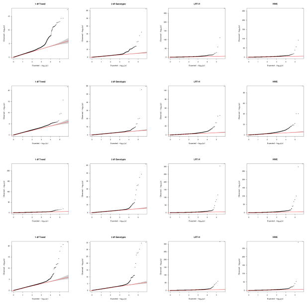
A genome-wide scan was conducted for each dataset with each of the four tests applied to each SNP. The corresponding Q-Q plots are shown in Figure 1, confirming no obvious population structures, as supported by the estimated inflation factors all close to 1 (Table 3).

Figure 1.

Q-Q plots of various tests for CD (first row), BD (2nd row), CAD (3rd row) and T2D (bottom row).

Table 3.

The inflation factors of various tests.

	CD	BD	CAD	T2D
1 df GLM	1.11	1.12	1.07	1.08
2 df GLM	1.09	1.10	1.07	1.07
LRT-H	1.13	1.13	1.09	1.10
HWE	0.96	0.97	0.98	0.97

After identifying significant SNPs at the usual genome-wide significance level of 5 × 10⁻⁸, we applied the method of Psychiatric Genomics Consortium (PGC, 2014) to define LD-independent (index) SNPs and risk loci. Briefly, first, among all significant SNPs, an SNP is defined to be an LD-independent SNP if it is in weak LD with r² < 0.1 with a more significant SNP within a 0.5Mb window; second, a risk locus is defined as a basepair (BP) interval including all the SNPs with r² > 0.6 to an LD-independent SNP, and any two risk loci within the distance of 0.25Mb are merged.

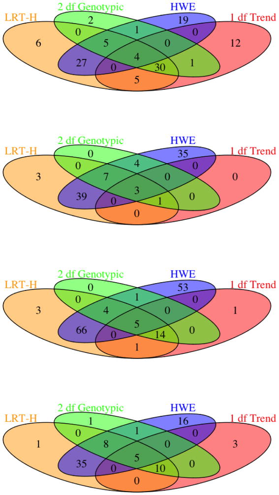
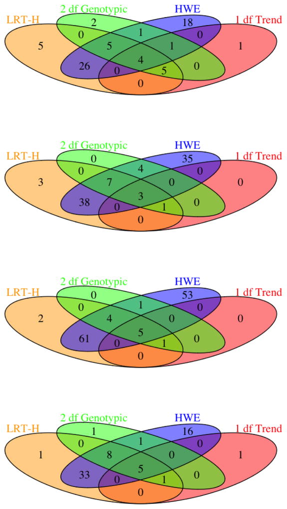
The numbers of significant SNPs and risk loci identified by each test are shown in Figures 2 and 3. It is clear that HWE test identified the largest numbers of significant SNPs and risk loci, most of which overlapped with those of the LRT-H test; this can be explained by the close connection between the two tests: a binomial mixture model implies the Hardy-Weinberg disequilibrium. Second, by the close relationship between the binomial mixture model and the expanded regression model (2), most of the significant SNPs and risk loci identified by the 2df test were also uncovered by the LRT-H test. Third, perhaps most importantly, since the LRT-H test also contrasts the allele frequency differences between the case and control groups as does the 1df trend test, the significant SNPs and risk loci identified by the popular trend test were almost all recovered by the LRT-H test. Finally, the LRT-H test also discovered some unique significant SNPs and risk loci.

Figure 2.

Venn-diagrams of the significant SNPs at the genome-wide significance level of 5 × 10⁻⁸ identified by each test for traits CD, BD, CAD and T2D (from the top to the bottom).

Figure 3.

Venn-diagrams of the significant risk loci identified by each test for traits CD, BD, CAD and T2D (from the top to the bottom).

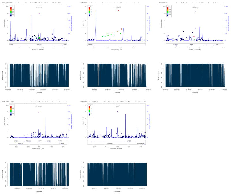
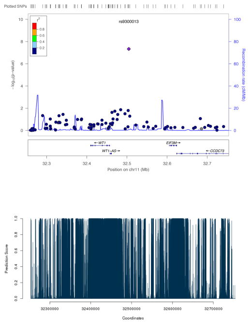
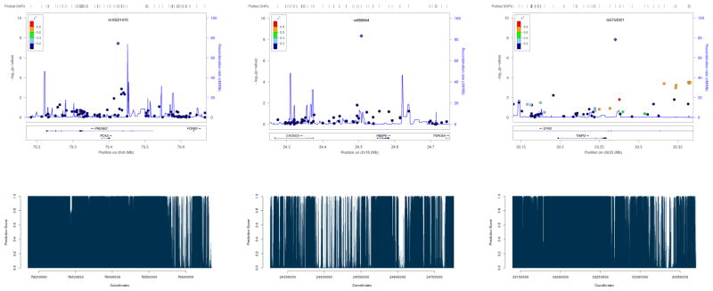
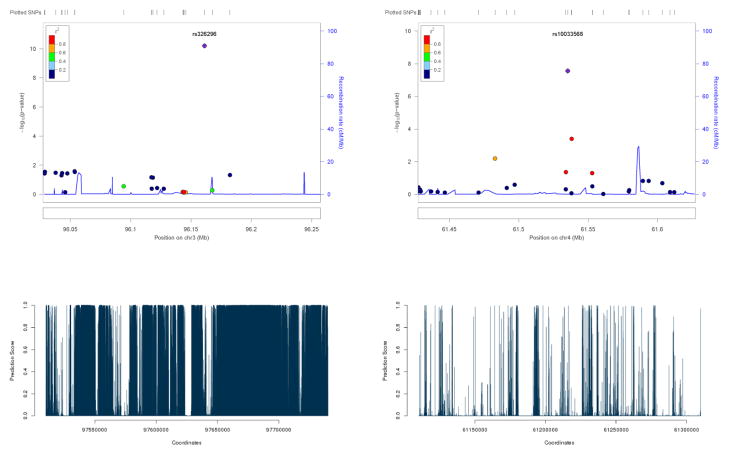
Some example SNPs identified to be significant by LRT-H, but not by other tests, are shown in Table 4. Some significant risk loci identified by the LRT-H or HWE test, but not by the other two tests, are confirmed to be within 0.25 Mb of some previously identified SNPs or risk loci, as shown in Table 5. The LocusZoom plots (Pruim et al 2010) for the significant risk loci uniquely identified by LRT-H are shown in Figures 4 – 7. To facilitate interpretation, we also added their predicted GenoCanyon scores (Lu et al 2015); a higher score predicts a higher likelihood of the SNP’s being functional. As GenoCanyon only supports hg19 while the original WTCCC data were all based on hg18, we lifted the annotation for the WTCCC data to hg19 using the UCSC web interface (http://genome.ucsc.edu/cgi-bin/hgLiftOver) before generating LocusZoom and GenoCanyon plots. We can see that some of the significant risk loci are in the regions with high functional scores.

Table 4.

Example SNPs which are identified to be significant by LRT-H, but not by HWE, 1 df Trend or 2 df Genotypic test.

Disease	SNP	CHR	BP	LRT-H	1 df Trend	2 df Genotypic	HWE
CD	rs6677092	1	238239905	1.35e-08	2.50e-04	9.51e-07	4.45e-06
BD	rs5754321	22	31600461	1.49e-08	5.31e-03	4.51e-03	2.47e-07
CAD	rs326296	3	97643917	6.28e-11	1.40e-05	2.39e-06	4.87e-07
T2D	rs9300013	11	32461118	4.62e-08	7.16e-03	2.58e-02	6.35e-07

Table 5.

Some significant risk loci identified by HWE or LRT-H, but not by the other two tests. Each risk locus is within 250 Kb of some previously identified SNPs or loci. For each risk locus, the LD-independent SNP along with the MAF in the control group and the p-values of LRT-H (P_LRT-H) and the HWE exact test (P_HWE) are reported.

Disease	CHR	SNP	BP (in Mb)	MAFcontrol	PLRT-H	PHWE	Reported genes	Ref
CD	3	rs12714959	18.59–18.62	0.304	4.04e-05	1.51e-09	-	Franke et al (2010)
	21	rs2252931	33.61–33.63	0.266	3.07e-01	3.41e-09	IFNGR2	Jostins et al (2012)
BD	6	rs7771567	97.81–98.01	0.301	7.41e-12	1.86e-11	MIR2113/POU3F2	Mühleisen et al (2014)
T2D	3	rs2377104	185.942570	0.491	9.57e-09	2.25e-09	IGF2BP2	Hara et al (2014)
	9	rs7030479	4.202347	0.066	1.28e-12	2.26e-13	GLIS3	Mahajan et al (2014)
	11	rs1002227	17.35–17.36	0.302	3.70e-08	1.29e-08	KCNJ11	Mahajan et al (2014)
	16	rs1350889	81.342–81.345	0.478	4.79e-10	1.16e-10	CMIP	Cho et al (2012)

Figure 4.

LocusZoom plots of the risk loci for trait CD, uniquely identified by LRT-H. The GenoCanyon scores for the LD-independent (index) SNPs are 2.71e-05, 5.3e-04, 1.00, 2.4e-03 and 5.5e-03 respectively.

Figure 7.

LocusZoom plot of the risk locus for trait T2D, uniquely identified by LRT-H. The GenoCanyon score for the LD-independent (index) SNP is 5.34e-05.

4 Discussion

We have shown possible power gain of the proposed LRT-H test which is closely related to the Hardy-Weinberg equilibrium (HWE) test. Briefly speaking, when applied to the WTCCC GWAS data, we found that the HWE test on the case group could identify the largest number of associated SNPs and risk loci for each of the four diseases considered, most of which overlapped with those of LRT-H, though LRT-H could uniquely detect some risk loci too. Although the HWE test has long been proposed as a possible choice for association testing (Nielsen et al 1998; Wittke-Thompson et al 2005), it has seldom been used and “often under-exploited” (Balding 2006) for such a purpose but most widely used only for SNP genotyping quality control. It is likely that some of the significant SNPs identified by the HWE test and LRT-H are due to genotyping errors, but some may be true positives. A challenge is to validate and interpret them as for any new discovery in GWAS.

R code will be available on the corresponding author’s website (http://www.biostat.umn.edu/~weip/prog.html).

Figure 5.

LocusZoom plots of the risk loci for trait BD, uniquely identified by LRT-H. The GenoCanyon scores for the LD-independent (index) SNPs are 0.999, 0.888 and 0.972 respectively.

Figure 6.

LocusZoom plots of the risk loci for trait CAD, uniquely identified by LRT-H. The GenoCanyon scores for the LD-independent (index) SNPs are 3.35e-06 and 1.24e-06 respectively.

References

- Balding DJ. A tutorial on statistical methods for population association studies. Nature Reviews Genetics. 2006;7:781–791. doi: 10.1038/nrg1916. [DOI] [PubMed] [Google Scholar]
- Burton PR, Clayton DG, Cardon LR, Craddock N, Deloukas P, Duncanson A, Kwiatkowski PD, McCarthy IM, Ouwehand HW, Samani JN, Todd AJ, Donnelly P. Genome-wide association study of 14,000 cases of seven common diseases and 3,000 shared controls. Nature. 2007;447(7145):661–678. doi: 10.1038/nature05911. [DOI] [PMC free article] [PubMed] [Google Scholar]
- Cho YS, Chen CH, Hu C, Long J, Ong RTH, Sim X, … McCarthy MI. Meta-analysis of genome-wide association studies identifies eight new loci for type 2 diabetes in east Asians. Nature Genetics. 2012;44(1):67–72. doi: 10.1038/ng.1019. [DOI] [PMC free article] [PubMed] [Google Scholar]
- Clayton D. In: Handbook of Statistical Genetics. Balding DJ, Bishop M, Cannings C, editors. Wiley; New York: 2003. pp. 939–960. [Google Scholar]
- Clayton D, Chapman J, Cooper J. Use of unphased multilocus genotype data in indirect association studies. Genetic Epidemiology. 2004;27(4):415–428. doi: 10.1002/gepi.20032. [DOI] [PubMed] [Google Scholar]
- Darabi H, Humphreys K. Single- and multi-locus association tests incorporating phenotype heterogeneity. Human Heredity. 2011;71(1):11–22. doi: 10.1159/000323750. [DOI] [PubMed] [Google Scholar]
- Erdmann J, Großhennig A, Braund PS, König IR, Hengstenberg C, Hall AS, … Meisinger C. New susceptibility locus for coronary artery disease on chromosome 3q22.3. Nature Genetics. 2009;41(3):280–282. doi: 10.1038/ng.307. [DOI] [PMC free article] [PubMed] [Google Scholar]
- Fan R, Knapp M. Genome association studies of complex diseases by case-control designs. American Journal of Human Genetics. 2003;72:850–868. doi: 10.1086/373966. [DOI] [PMC free article] [PubMed] [Google Scholar]
- Franke A, McGovern DP, Barrett JC, Wang K, Radford-Smith GL, Ahmad T, … Parkes Miles. Genome-wide meta-analysis increases to 71 the number of confirmed Crohn’s disease susceptibility loci. Nature Genetics. 2010;42(12):1118–1125. doi: 10.1038/ng.717. [DOI] [PMC free article] [PubMed] [Google Scholar]
- Galvan A, Ioannidis JP, Dragani TA. Beyond genome-wide association studies: genetic heterogeneity and individual predisposition to cancer. Trends in Genetics. 2010;26(3):132–141. doi: 10.1016/j.tig.2009.12.008. [DOI] [PMC free article] [PubMed] [Google Scholar]
- Hara K, Fujita H, Johnson TA, Yamauchi T, Yasuda K, Horikoshi M, … Kadowaki T. Genome-wide association study identifies three novel loci for type 2 diabetes. Human Molecular Genetics. 2014;23(1):239–246. doi: 10.1093/hmg/ddt399. [DOI] [PubMed] [Google Scholar]
- Jostins L, Ripke S, Weersma RK, Duerr RH, McGovern DP, Hui KY, … Hart A. Host-microbe interactions have shaped the genetic architecture of inflammatory bowel disease. Nature. 2012;491(7422):119–124. doi: 10.1038/nature11582. [DOI] [PMC free article] [PubMed] [Google Scholar]
- Kathiresan S, Voight BF, Purcell S, Musunuru K, Ardissino D, Mannucci PM, … Ramos R. Genome-wide association of early-onset myocardial infarction with single nucleotide polymorphisms and copy number variants. Nature Genetics. 2009;41(3):334–341. doi: 10.1038/ng.327. [DOI] [PMC free article] [PubMed] [Google Scholar]
- Kim S, Morris NJ, Won S, Elston RC. Single-marker and two-marker association tests for unphased casecontrol genotype data, with a power comparison. Genetic Epidemiology. 2010;34(1):67–77. doi: 10.1002/gepi.20436. [DOI] [PMC free article] [PubMed] [Google Scholar]
- Londono D, Buyske S, Finch SJ, Sharma S, Wise CA, Gordon D. TDT-HET: a new transmission disequilibrium test that incorporates locus heterogeneity into the analysis of family-based association data. BMC Bioinformatics. 2012;13(1):13. doi: 10.1186/1471-2105-13-13. [DOI] [PMC free article] [PubMed] [Google Scholar]
- Lu Q, Hu Y, Sun J, Cheng Y, Cheung KH, Zhao H. A statistical framework to predict functional non-coding regions in the human genome through integrated analysis of annotation data. Scientific Reports. 2015;5 doi: 10.1038/srep10576. [DOI] [PMC free article] [PubMed] [Google Scholar]
- Mahajan A, Go MJ, Zhang W, Below JE, Gaulton KJ, Ferreira T, … Chidambaram M. Genome-wide trans-ancestry meta-analysis provides insight into the genetic architecture of type 2 diabetes susceptibility. Nature Genetics. 2014;46(3):234–244. doi: 10.1038/ng.2897. [DOI] [PMC free article] [PubMed] [Google Scholar]
- McClellan J, King MC. Genetic heterogeneity in human disease. Cell. 2010;141(2):210–217. doi: 10.1016/j.cell.2010.03.032. [DOI] [PubMed] [Google Scholar]
- Mühleisen TW, Leber M, Schulze TG, Strohmaier J, Degenhardt F, Treutlein J, Alda M. Genome-wide association study reveals two new risk loci for bipolar disorder. Nature Communications. 2014;5 doi: 10.1038/ncomms4339. [DOI] [PubMed] [Google Scholar]
- Nielsen DM, Ehm MG, Weir BS. Detecting marker-disease association by testing for Hardy-Weinberg disequilibrium at a marker locus. American Journal of Human Genetics. 1998;63(5):1531–1540. doi: 10.1086/302114. [DOI] [PMC free article] [PubMed] [Google Scholar]
- Pan W. Asymptotic tests of association with multiple SNPs in linkage disequilibrium. Genetic Epidemiology. 2009;33(6):497. doi: 10.1002/gepi.20402. [DOI] [PMC free article] [PubMed] [Google Scholar]
- Pruim RJ, Welch RP, Sanna S, Teslovich TM, Chines PS, Gliedt TP, Boehnke M, Abecasis GR, Willer CJ. LocusZoom: regional visualization of genome-wide association scan results. Bioinformatics. 2010;26(18):2336–2337. doi: 10.1093/bioinformatics/btq419. [DOI] [PMC free article] [PubMed] [Google Scholar]
- Qian M, Shao Y. A likelihood ratio test for genomewide association under genetic heterogeneity. Annals of Human Genetics. 2013;77(2):174–182. doi: 10.1111/ahg.12005. [DOI] [PMC free article] [PubMed] [Google Scholar]
- Samani NJ, Erdmann J, Hall AS, Hengstenberg C, Mangino M, Mayer B, … Schunkert H. Genomewide association analysis of coronary artery disease. New England Journal of Medicine. 2007;357(5):443–453. doi: 10.1056/NEJMoa072366. [DOI] [PMC free article] [PubMed] [Google Scholar]
- Schizophrenia Working Group of the Psychiatric Genomics Consortium. Biological insights from 108 schizophrenia-associated genetic loci. Nature. 2014;511(7510):421–427. doi: 10.1038/nature13595. [DOI] [PMC free article] [PubMed] [Google Scholar]
- Scott LJ, Mohlke KL, Bonnycastle LL, Willer CJ, Li Y, Duren WL, … Boehnke M. A genome-wide association study of type 2 diabetes in Finns detects multiple susceptibility variants. Science. 2007;316(5829):1341–1345. doi: 10.1126/science.1142382. [DOI] [PMC free article] [PubMed] [Google Scholar]
- Schunkert H, König IR, Kathiresan S, Reilly MP, Assimes TL, Holm H, … Samani NJ. Large-scale association analysis identifies 13 new susceptibility loci for coronary artery disease. Nature Genetics. 2011;43(4):333–338. doi: 10.1038/ng.784. [DOI] [PMC free article] [PubMed] [Google Scholar]
- Sasieni PD. From genotypes to genes: doubling the sample size. Biometrics. 1997:1253–1261. [PubMed] [Google Scholar]
- Wellek S, Ziegler A. Cochran-Armitage test versus logistic regression in the analysis of genetic association studies. Human Heredity. 2012;73(1):14–17. doi: 10.1159/000334085. [DOI] [PubMed] [Google Scholar]
- Wigginton JE, Cutler DJ, Abecasis GR. A note on exact tests of Hardy-Weinberg equilibrium. American Journal of Human Genetics. 2005;76:887–93. doi: 10.1086/429864. [DOI] [PMC free article] [PubMed] [Google Scholar]
- Wittke-Thompson JK, Pluzhnikov A, Cox NJ. Rational inferences about departures from Hardy-Weinberg equilibrium. American Journal of Human Genetics. 2005;76:967–986. doi: 10.1086/430507. [DOI] [PMC free article] [PubMed] [Google Scholar]
- Zhou H, Pan W. Binomial mixture model-based association tests under genetic heterogeneity. Annals of Human Genetics. 2009;73(6):614–630. doi: 10.1111/j.1469-1809.2009.00542.x. [DOI] [PMC free article] [PubMed] [Google Scholar]
- Xiong M, Zhao J, Boerwinkle E. Generalized T2 test for genome association studies. American Journal of Human Genetics. 2002;70:1257–1268. doi: 10.1086/340392. [DOI] [PMC free article] [PubMed] [Google Scholar]