RACOG and wRACOG: Two Probabilistic Oversampling Techniques

Abstract

As machine learning techniques mature and are used to tackle complex scientific problems, challenges arise such as the imbalanced class distribution problem, where one of the target class labels is under-represented in comparison with other classes. Existing oversampling approaches for addressing this problem typically do not consider the probability distribution of the minority class while synthetically generating new samples. As a result, the minority class is not well represented which leads to high misclassification error. We introduce two Gibbs sampling-based oversampling approaches, namely RACOG and wRACOG, to synthetically generating and strategically selecting new minority class samples. The Gibbs sampler uses the joint probability distribution of attributes of the data to generate new minority class samples in the form of Markov chain. While RACOG selects samples from the Markov chain based on a predefined lag, wRACOG selects those samples that have the highest probability of being misclassified by the existing learning model. We validate our approach using five UCI datasets that were carefully modified to exhibit class imbalance and one new application domain dataset with inherent extreme class imbalance. In addition, we compare the classification performance of the proposed methods with three other existing resampling techniques.

1 Introduction

With a wide spectrum of industries drilling down into their data stores to collect previously unused data, data are being treated as the “new oil”. Social media, healthcare, and e-commerce companies are refining and analyzing data with the goal of creating new products and/or adding value to existing ones. As machine learning techniques mature and are used to tackle scientific problems in the current deluge of data, a variety of challenges arise due to the nature of the underlying data. One well-recognized challenge is the imbalanced class distribution problem, where one of the target classes (the minority class) is under-represented in comparison with the other classes (the majority class or classes).

While many datasets do not contain a perfectly uniform distribution among class labels, some distributions contain less than 10% minority class data samples, which is considered imbalanced. Because the goal of supervised learning algorithms or classifiers is to optimize prediction accuracy for the entire data set, most approaches ignore performance on the individual class labels. Therefore, a random classifier that labels all data samples from an imbalanced class dataset as members of the majority class would become the highest performing algorithm despite incorrectly classifying all minority class samples. However, in many problem domains such as cancerous cell identification [1], oil-spill detection [2], fraud detection [3], keyword extraction [4], and text classification [5], identifying members of the minority class is critical, sometimes more so than achieving optimal overall accuracy for the majority class.

The imbalance class distribution problem has vexed researchers for over a decade and has thus received focused attention. The common techniques that have been investigated include: Resampling, which balances class priors of training data by either increasing the number of minority class data samples (oversampling) or decreasing the number of majority class data samples (undersampling); cost-sensitive learning, which assigns higher misclassfication cost for minority class samples than majority class; and, kernel-based learning methods, which make the minority class samples more separable from the majority class by mapping the data to a high dimensional feature space. Among these techniques, resampling methods remain at the forefront due to their ease of implementation. Liu et al. [6] articulate a number of reasons to prefer resampling to other methods. First, because resampling occurs during preprocessing, the approach can be combined with others such as cost-sensitive learning, without changing the algorithmic anatomy [7]. Second, theoretical connections between resampling and cost-sensitive learning indicate that resampling can alter the misclassification costs of data points [8]. Third, empirical evidence demonstrates nearly identical performance between resampling and cost-sensitive learning techniques [9], [10].

Although both under- and over-sampling techniques have been improving over the years, we focus our attention on oversampling because it is well suited for the application that motivates our investigation. Because many class imbalance problems involve an absolute rarity of minority class data samples [11], undersampling of majority class examples is not advisable. However, we use an undersampling method, RUSBoost [12], as a proof of concept to compare with the proposed Gibbs sampling-based oversampling techniques: RACOG and wRACOG.

Existing oversampling approaches [13], [14] that add synthetic data to alleviate class imbalance problem typically rely on spatial location of minority class samples in the Euclidean feature space. These approaches harvest local information of minority class samples to generate new synthetic samples that are also assumed to belong to the minority class. Although this approach may be acceptable for data sets where a crisp decision boundary exists between the classes, spatial location-based synthetic oversampling is not suitable for data sets that have overlap between the minority and majority classes. Therefore, a better idea is to exploit global information of minority class samples, which can be done by considering the probability distribution of minority class while synthetically generating new minority class samples.

In this paper, we exploit advances in the area of Markov chain Monte Carlo (MCMC) methods to introduce two Gibbs sampling-based oversampling approaches, called RACOG and wRACOG, to generating and strategically selecting new minority class data points. Specifically, the proposed algorithms generate new minority class data points via Gibbs sampling by exploiting the joint probability distribution and interdependencies of attributes. While RACOG selects samples from the Markov chain generated by the Gibbs sampler using a predefined lag, wRACOG selects those samples that have the highest probability of being misclassified by the existing learning model.

We validate our approach using five UCI datasets, carefully modified to exhibit class imbalance, and one new application domain dataset² with inherent extreme class imbalance. The proposed methods, RACOG and wRACOG are compared with two existing oversampling techniques, SMOTE [13] and SMOTEBoost [14] and an undersampling technique RUSBoost [12]. We evaluate the alternative approaches using the performance measures Sensitivity, G-mean, and Area Under ROC Curve (AUC-ROC).

2 Related Work

Learning from class imbalanced datasets is a niche, yet critical area in supervised machine learning due to its increased prevalence in real world problem applications [15], [16], [17], [18]. Due to the pervasive nature of the imbalanced class problem, a wide spectrum of related techniques has been proposed. One of the most common solutions that has been investigated is cost sensitive learning (CSL). CSL methods counter the underlying assumption that all errors are equal by introducing customized costs for misclassifying data points. By assigning a sufficiently high cost to minority sample points, the algorithm may devote sufficient attention to these points to learn an effective class boundary. The effectiveness of CSL methods has been validated theoretically [8], [10] and empirically [9], [19], although other studies indicate that there is no clear winner between CSL and other methods such as resampling [20]. In addition, CSL concepts have been coupled with existing learning methods to boost their performance [21], [22], [23]. CSL approaches do have drawbacks that limit their application. First, the misclassification costs are often unknown or need to be painstakingly determined for each application. Second, not all learning algorithms have cost sensitive implementation.

A second direction is to adapt the underlying classification algorithm to consider imbalanced classes, typically using kernel-based learning methods. Since kernel-based methods provide state-of-the-art techniques for many machine learning applications, using them to understand the imbalanced learning problem has attracted increased attention. The kernel classifier construction algorithm proposed by Hong et al. [24] is based on orthogonal forward selection and a regularized orthogonal weighted least squares (ROWLSs) estimator. Wu et al. [25] propose a kernel-boundary alignment (KBA) algorithm for adjusting the SVM class boundary. KBA is based on the idea of modifying the kernel matrix generated by a kernel function according to the imbalanced data distribution. Another interesting kernel modification technique is the k-category proximal support vector machine (PSVM) [26] proposed by Fung et al. This method transforms the soft-margin maximization paradigm into a simple system of k-linear equations for either linear or nonlinear classifiers.

Probably the most common approach, however, is to resample, or modify the dataset in a way that balances the class distribution. Determining the ideal class distribution is an open problem [21] and in most cases it is handled empirically. Naive resampling methods include oversampling the minority class by duplicating existing data points and undersampling the majority class by removing chosen data points. However, random over-sampling and under-sampling increases the possibility of overfitting and discarding useful information from the data, respectively.

An intelligent way of oversampling is to synthetically generate new minority class samples. Synthetic minority class oversampling technique, or SMOTE [13], has shown a great deal of success in various application domains. SMOTE oversamples the minority class by taking each minority class data point and introducing synthetic examples along the line segments joining any or all of the k-minority class nearest neighbors. In addition, adaptive synthetic sampling techniques have been introduced that take a more strategic approach to selecting the set of those minority class samples on which synthetic oversampling should be performed. For example, Borderline-SMOTE [27] generates synthetic samples only for those minority class examples that are “closer” to the decision boundary between the two classes. ADASYN [28], on the other hand, uses the density distribution of the minority class samples as a criterion to automatically decide the number of synthetic samples that need to be generated for each minority example by adaptively changing the weights of different minority examples to compensate for the skewed distribution. Furthermore, class imbalance problems associated with intra-class imbalanced distribution of data in addition to inter-class imbalance can be handled by cluster-based oversampling (CBO) proposed by Jo et al. [29].

The information loss incurred by random under-sampling can be overcome by methods to strategically remove minority class samples. Liu et al. [30] proposed two informed undersampling techniques that use ensembles to learn from majority class subsets. For data sets that have overlapping minority and majority classes [31], data cleansing is used to minimize unwanted overlapping between classes by removing pairs of minimally distanced nearest neighbors of opposite classes, popularly known as Tomek links [32], [33], [34]. Because removing Tomek links changes the distribution of the data, it might not be beneficial in situations when there is a dense overlap between the classes, because this approach might lead to overfit. There are additionally ensemble learning approaches [35] that combine the powers of resampling and ensemble learning. These approaches include, but are not restricted to, SMOTEBoost [14], RUSBoost [12], IVotes [36] and SMOTE-Bagging [37].

Empirical studies [20] have shown that approaches such as cost sensitive learning or kernel-based learning are not quite suitable for class imbalanced data sets that have “rare” minority class samples. Also, any form of under-sampling witnesses the same problem. We are interested in applying supervised learning techniques to a dataset that includes rare minority class samples. While oversampling is a natural solution to this problem, existing oversampling techniques such as SMOTE, Borderline-SMOTE and SMOTEBoost generate new data samples that are spatially close to existing minority class examples in the Euclidean feature space. Ideally new data samples should be representative of the entire minority class and not just be drawn from local information. Therefore, in this paper we focus on satisfying the criteria of global representation of the minority class by generating multivariate samples from the joint probability distribution of the underlying random variables or attributes.

3 Application Domains

We are motivated to pursue this challenge by a problem in pervasive computing. Specifically, we are designing smart environments that perform health monitoring and assistance. Studies have shown that smart environment technologies can detect errors in activity completion and might be utilized to extend independent living in one’s own home without compromising safety [38], [39]. One type of intervention that is valuable for individuals with cognitive impairment is automated prompts that aid with activity initiation and completion.

Rule-based approaches to prompting individuals for activity initiation or completion have been developed by gerontechnology researchers [40], [41]. However, cognitive rehability theory indicates that combining prompting technology with knowledge of activity and cognitive context are valuable for effective health promotion [40], [42]. We postulate that prompt timing can be automated by incorporating contextual information provided by a smart home.

To determine the ability of a machine learning algorithm to generate appropriate activity-aware prompts, we performed a study in our smart home with 128 volunteer participants, aged 50+, who are healthy older adults or individuals with mild cognitive impairment. The smart home is a two-story apartment equipped with sensors that monitor motion, door open/shut status, and usage of water, burner, and specific items throughout the apartment.

Clinically-trained psychologists watch over a web camera as the participants perform 8 different activities. The psychology experimenter remotely issues a prompt when they determine that the individual is having difficulty initiating or completing an activity. Sensor events, denoted by the event date, time, sensor identifier, and message, are collected continuously, along with the prompt timings. A human annotator annotates the sensor events with corresponding activity and a sub-step that act as the ground truth. Table 1 shows a snippet of annotated events. On the basis of ground truth information, the feature vector for every activity sub-step present in the database is generated that consists of temporal, spatial and contextual features. We can view automated prompting as a supervised learning problem in which each activity step is mapped to a “Prompt” or “No-prompt” class label. Thus, automated prompting emulates natural interventions provided by a caregiver.

TABLE 1.

Human Annotated Sensor Events

Date	Time	SensorID	Status	Annotation	Prompt
2009-05-11	14:59:54	D010	CLOSE	cook-3	prompt
2009-05-11	14:59:55	M017	ON	cook-4	no-prompt
2009-05-11	15:00:02	M017	OFF	none	no-prompt
2009-05-11	15:00:17	M017	ON	cook-8	no-prompt
2009-05-11	15:00:34	M018	ON	cook-8	no-prompt
2009-05-11	15:00:35	M051	ON	cook-8	no-prompt
2009-05-11	15:00:43	M016	ON	cook-8	no-prompt
2009-05-11	15:00:43	M015	ON	cook-9	no-prompt
2009-05-11	15:00:45	M014	ON	cook-9	no-prompt

The prompting dataset, as we would like to call it, has 3980 examples with 17 features. Out of the 17 features, 4 are categorical and the rest are numeric. The difficulty that is faced for the prompting problem is that the majority of activity steps are “no-prompt” cases and standard machine learning algorithms will likely map all data points to this class, which defeats the purpose of the intervention. Our goal is to design solutions to the class imbalance problem that improve sensitivity for this prompting application.

We evaluate the applicability of our algorithm for other datasets by evaluating them on five additional real-world datasets from the UCI repository that exhibit the class imbalance problem: abalone, car, nursery, letter, and connect-4. Characteristics of these datasets are summarized in Table 2. The real-valued attributes were transformed into discrete sets by using a simple binning technique. The multi-class datasets were converted into binary class by choosing a particular class label as minority class and the rest of the class labels together as majority class.

TABLE 2.

Description of selected datasets

Dataset	Size	Dim	% Min. Class	Description
Prompting	3,980	17	3.7437	Description in Section 3.
Abalone	4,177	8	6.2006	Predicting age of large sea snails, abalone, from its physical measurements.
Car	1,728	6	3.9931	Evaluating car acceptability based on price, technology and comfort.
Nursery	12,960	8	2.5463	Nursery school application evaluation based on financial standing, parents’ education and social health.
Letter	20,000	16	3.7902	Classifying English alphabets using image frame features.
Connect-4	5000	42	10.0000	Predicting first player’s outcome in connect-4 game given 8-ply positions information.

4 Proposed Approaches: RACOG and wRACOG

Our proposed approaches to oversampling for imbalanced class distribution is based upon Gibbs sampling. Gibbs sampling is rooted in image processing and was introduced by Geman and Geman (1984). The family of Markov chain Monte Carlo (MCMC) methods, of which Gibbs sampling is a type, originated with the Metropolis algorithm [43], [44]. Before discussing about Gibbs sampling and the way we have used it to design RACOG and wRACOG, it is useful to give a brief introduction to Markov chains which forms the basis of any MCMC technique.

A first-order Markov chain is defined to be a series of random variables z⁽¹⁾, …, z^(M), such that the conditional independence property given in Equation 1 holds true for m ∈ {1, .., M − 1}.

$$P(z^{(m+1)}\mid z^{(1)},\mathrm{..},z^{(m)})=P(z^{(m+1)}\mid z^{(m)})$$ (1)

This can be represented as a directed graph in the form of a chain as shown in Figure 1. The Markov chain can then be specified by giving the probability distribution of the initial variable P (z⁽⁰⁾) and the conditional probabilities of the subsequent variables (transition probabilities).

Fig. 1.

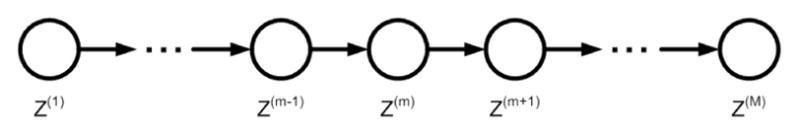
A Markov chain

Thus, the marginal probability of a variable of interest can be expressed in terms of the marginal probability of the previous variable and the transition probability from the previous variable to the current variable (see Equation 2).

$$P(z^{(m+1)})=\sum _{z^{(m)}}P(z^{(m+1)}\mid z^{(m)})P(z^{(m)})$$ (2)

4.1 Standard Gibbs Sampler

The goal of a Gibbs sampler is to generate a Markov chain, sometimes referred as Gibbs sequence in Gibbs sampling context, whose samples converge to the target distribution. The approach is applicable in situations where the random variable Z has at least two dimensions (z =< z₁, .., z_k >, k > 1). At each sampling step, the algorithm considers univariate conditional distributions where each of the dimensions but one is assigned a fixed value. Rather than picking the entire collection of attribute values at once, a separate probabilistic choice is made for each of the k dimensions, where each choice depends on the values of the other k − 1 dimensions and the previous value of the same dimension. Such conditional distributions are easier to model than the full joint distribution. Figure 2 shows the algorithm for the standard Gibbs sampler. As we would find later in this section, we exploit the univariate conditional distribution of each dimension, represented by $P\left(Z_i\mid z_1^{(t+1)},\dots ,z_{i-1}^{(t+1)},z_{i+1}^{(t)},\dots ,z_k^{(t)}\right)$ to probabilistically choose attribute values that form a new synthetically generated sample.

Fig. 2.

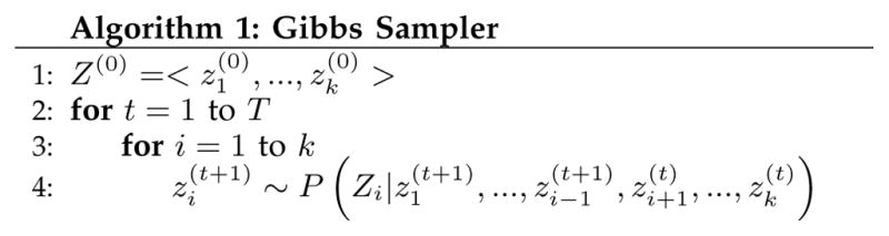
Gibbs Sampling

Implementations of Gibbs samplers are traditionally dependent on two factors. The first is the number of sample generation iterations that are needed for the samples to reach a stationary distribution (i.e., when the marginal distribution of Z⁽ⁿ⁾ is independent of n). In order to avoid the estimates being contaminated by values at iterations before this point (referred to as the burn-in), earlier samples are discarded. The second factor is that a sample generated during one iteration is highly dependent on the previous sample. This correlation between successive values, or autocorrelation, is avoided by defining a suitable lag, or number of consecutive samples to discard from the Markov chain following each accepted generated sample.

4.2 The RACOG Algorithm

The RApidy COnverging Gibbs sampler (RACOG) uses Gibbs sampling at its core to generate new minority class samples from the distribution of the minority class. RACOG enhances standard Gibbs sampling by offering an alternative mechanism for choosing the initial values of the random variable Z (denoted by Z⁽⁰⁾), that help generate samples which rapidly converge to the target (minority class) distribution, and by imposing dependencies among the attributes which form the k dimensions of the random variable.

Conventionally, the initial values of the random variable to “ignite” the Gibbs sampler are randomly chosen value in the state space of the attributes. This approach takes a high burn-in period and an extremely large number of iterations for the sampler to converge with the target distribution. On the other hand, RACOG chooses the minority class data points as the set of initial samples and runs the Gibbs sampler for every minority class example. The total number of iterations for the Gibbs sampler is restricted by the desired minority:majority class distribution. Thus, RACOG produces multiple Markov chains, each starting with a different minority class sample, instead of one very long chain as done in conventional Gibbs sampling. As the initial samples of RACOG are chosen directly from the minority class samples, it helps in achieving faster convergence of the generated samples with the minority class distribution. This claim is validated with the help of a convergence test performed in Section 6.

There are arguments in the literature about the pros and cons of single long Markov chain and multiple shorter chain approaches. Geyer [45] argues that a single long chain is a better approach because, if long burn-in periods are required, or if the chains have high autocorrelations, using a number of shorter chains may result in chains that are not long enough to be of any value in representing the minority class. However, single long chain requires very high number or iterations to converge with the target distribution. Our experiments show that the argument made by Geyer does not hold when multiple chains are generated with the minority class data points as the initial samples of the Gibbs sampler.

The last stumbling block in successful usage of Gibbs sampling is the conditional distribution mentioned in Step 4 of the algorithm (Figure 2) which is used to probabilistically determine attribute values for the new sample. Simplified version of the conditional distribution (see Equation 3) represents a ratio between joint probability of all attributes values of the random variable and a normalizing factor.

$$\frac{P\left(Z_i\mid z_1^{(t+1)},\dots ,z_{i-1}^{(t+1)},z_{i+1}^{(t)},\dots ,z_k^{(t)}\right)=P\left(z_1^{(t+1)},\dots ,z_{i-1}^{(t+1)},z_i^{(t)},z_{i+1}^{(t)},\dots ,z_k^{(t)}\right)}{P\left(z_1^{(t+1)},\dots ,z_{i-1}^{(t+1)},z_{i+1}^{(t)},\dots ,z_k^{(t)}\right)}$$ (3)

However, datasets which have extremely rare minority class samples and sufficiently high dimensional random variable, the probability of joint occurrences of other attribute values is extremely low due to insufficient number of such minority class samples. Because standard Gibbs Sampling algorithm does not impose dependencies on attributes of the random variables, sampling performed in Step 4 of the algorithm disallows exploration of the entire space of attributes and is therefore less likely to generate points that are consistent with such minority class distribution. On the other hand, considering a full joint distribution will be prone to error because there are insufficient minority points to accurately estimate the probabilities that are used in Equation 3.

The RACOG algorithm explores the state space of attributes more thoroughly by factoring the large-dimensional joint distribution into a directed acyclic graph (DAG) that imposes explicit dependencies between attributes. Thus, the probability of a particular data sample, x, represented as a collection of attributes {x_i : 1 ≤ i ≤ M}, is be computable as:

$$P(x)=\prod _{i}P(x_i\mid x_{\mathit{parents}(i)})$$ (4)

Traditionally, the DAG is constructed by learning a Bayesian network which uses search techniques, such as hill climbing or simulated annealing. An alternative, less computationally expensive approach, is to employ the Chow-Liu algorithm (1968) described in Figure 3, to construct a Bayesian tree of dependencies by reducing the problem of constructing a maximum likelihood tree to that of finding a maximal weighted spanning tree in a graph. RACOG employs this approach to finding a Bayesian tree among attribute dependencies. This allows each attribute (but the root) to have exactly one parent on which its value depends [46]. Figure 4 shows Bayesian trees formed from the abalone and car datasets. Attributes length and lug boot are chosen as the roots of the Bayesian trees for abalone and car, respectively. The number of children for the nodes gives us an insight into the importance of those attributes in the dataset. In other words, the greater branching factor of a node, the greater its importance. Equation 3 is now represented as:

$$P\left(Z_i\mid z_1^{(t+1)},\dots ,z_{i-1}^{(t+1)},z_{i+1}^{(t)},\dots ,z_k^{(t)}\right)=\frac{P\left(z_{\mathit{root}}{\prod }_{x}P(z_x\mid z_{\mathit{parents}(x)})\right)}{P\left(z_1^{(t+1)},\dots ,z_{i-1}^{(t+1)},z_{i+1}^{(t)},\dots ,z_k^{(t)}\right)}$$ (5)

Fig. 3.

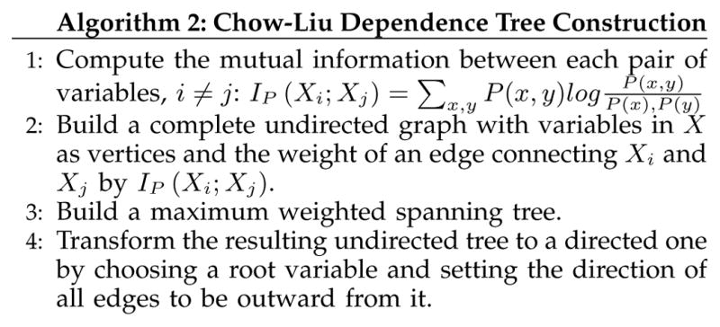
Chow-Liu Dependence Tree Construction

Fig. 4.

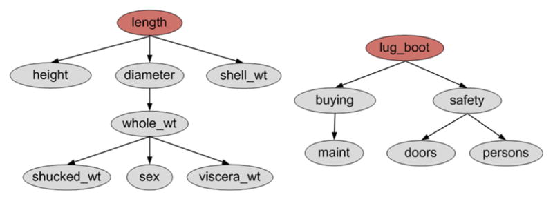
Trees for (left) abalone and (right) car datasets

Finally, to generate a new minority class sample, value of an attribute i represented by $z_i^{(t+1)}$ is determined by randomly sampling from the distribution of the state space (all possible values) of attribute i represented by $P\left(Z_i\mid z_1^{(t+1)},\dots ,z_{i-1}^{(t+1)},z_{i+1}^{(t)},\dots ,z_k^{(t)}\right)$. Figure 5 summarizes the RACOG algorithm.

Fig. 5.

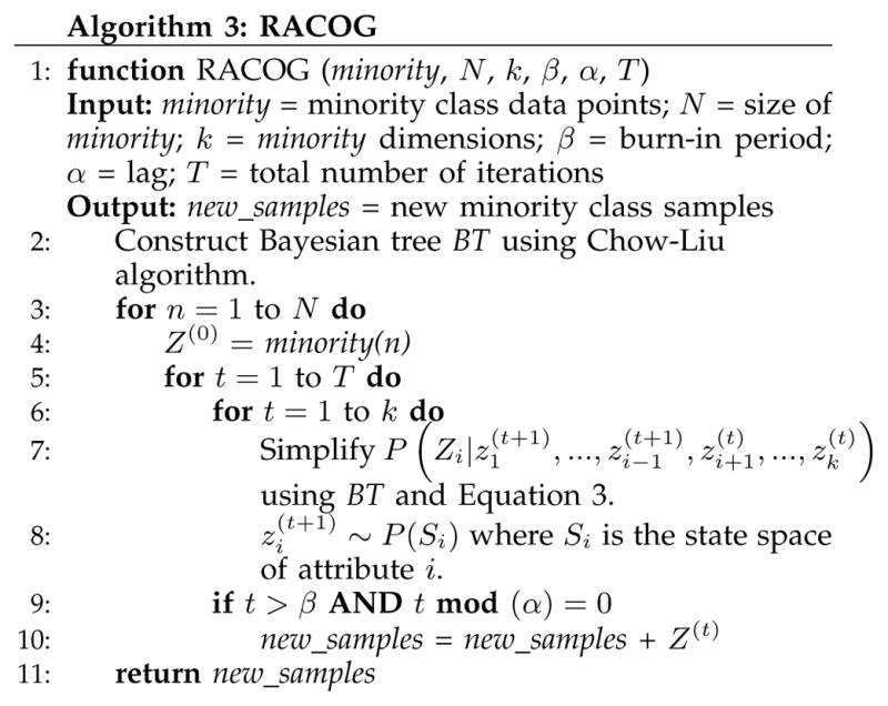
The RACOG Algorithm

While the RACOG algorithm enhances traditional Gibbs sampler by making it suitable for class imbalanced data, this approach does not take into account the usefulness of the generated samples. Thus, RACOG might add minority class samples that are redundant and have no contribution towards constructing a better hypothesis. In the next section, we introduce a wrapper enhancement to the RACOG algorithm that addresses this issue.

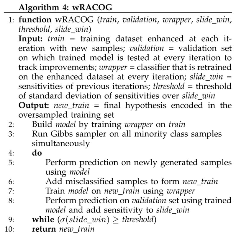
4.3 The wRACOG algorithm

The enhanced RACOG algorithm, named wRACOG, is a wrapper-based technique over RACOG utilizing Gibbs sampling as the core data sampler. However, the purpose of introducing wRACOG is to decouple the concept of burn-in and lag associated with sample selection from conventional Gibbs sampling. By performing iterative training on the dataset with newly generated samples, wRACOG selects those samples from the Markov chain that have the highest probability of being misclassified by the learning model generated from the previous version of the dataset.

While the RACOG algorithm generates minority class samples for a fixed (predefined) number of iterations, the wRACOG algorithm keeps on fine tuning its hypothesis at every iteration by adding new samples until there is no further improvement with respect to a chosen performance measure. As our goal is to improve the performance of classifiers on the minority class, wRACOG keeps on adding new samples until there is no further improvement in sensitivity (true positive rate) of the wrapper classifier (the core classifier that retrains at every iteration) of wRACOG. This process acts as the “stopping criterion” for the wRACOG algorithm. However, the choice of performance measure for the stopping criterion is application dependent.

At each iteration of wRACOG, new minority class samples are generated by the Gibbs sampler. The model learned by the wrapper classifier on the enhanced set of samples produced in the previous iteration is used to make predictions on the newly generated set of samples. Those samples that are misclassified by the model are added to the existing set of data samples and a new model is trained using the wrapper classifier. At each iteration, the trained model performs prediction on a held out validation set and the sensitivity of the model is recorded. Generation of new samples stops once the standard deviation of sensitivities over the past iterations falls below a threshold. As the wRACOG algorithm might end up running many iterations, the standard deviation of sensitivities is calculated over a fixed number of most recent iterations (slide win). We use the values slide win=10 and threshold=0.02 for our experiments, determined by performing an empirical study on the datasets described in this paper. The wRACOG algorithm is summarized in Figure 6.

Fig. 6.

The wRACOG Algorithm

Although wRACOG is similar to existing boosting techniques (such as AdaBoost) in the way misclassified samples are assigned higher weights to ensure they get selected during random sampling in the next boosting iteration, there are a number of major distinctions. Firstly, while in traditional boosting, both training and prediction are performed on the same set of data samples, wRACOG trains the current hypothesis on the data samples from the previous iteration and performs prediction only on the newly generated samples from the Gibbs sampler. Secondly, there is no concept of changing weights of the samples before resampling, as the newly generated samples are directly added to the existing set of samples. Thirdly, wRACOG does not use weighted voting of multiple hypotheses learned at every iteration. Instead, it employs multiple iterations to fine tune a single hypothesis. We hypothesize that by applying this approach we can reduce the generation of redundant samples to converge more closely to the true distribution of the minority class, and also reduce the overhead of generating multiple hypotheses as is employed by traditional boosting techniques.

Thus, usage of Gibbs sampler as the core component helps RACOG and wRACOG exploit global properties of the minority class and not just local distance between specific data points.

5 Experimental Setup

The goal of the current work is to design algorithms that effectively classify data points from all classes, even with imbalanced class distribution. We hypothesize that Gibbs sampling, particularly with additional modeling of attribute dependencies, will yield improved results for problems that exhibit class imbalance. To validate our hypothesis, we compare the results for alternative sampling algorithms using the datasets summarized in Table 2.

5.1 Alternative Sampling Approaches

While reporting the results for the experiments, six different methods are evaluated in order to validate the proposed hypothesis. The first method, named Baseline, relies upon the baseline dataset without any sampling or preprocessing. The evaluation is performed using the classifiers discussed in Section 5.2. Rest of the methods discussed in this section preprocess the baseline dataset.

5.1.1 SMOTE [13]

SMOTE is an oversampling approach in which the minority class is oversampled by creating “synthetic” examples based on spatial location of the data points in the Euclidean feature space. Oversampling is performed by considering each minority class data point and introducing synthetic examples along the line segments joining any or all of the k-minority class nearest neighbors. The k-nearest neighbors are randomly chosen depending upon the amount of oversampling required. Synthetic data points are generated in the following way: First, the difference between the data point under consideration and its nearest neighbor is computed. This difference is multiplied by a random number between 0 and 1, and it is added to the data point under consideration. This results in the selection of a random point in the Euclidean space, along the line segment between two specific data points. Consequently, by adding diversity to the minority class, this approach forces the decision boundary between the two regions to be crisper. However, as SMOTE does not rely on the probability distribution of the minority class as a whole, there is no guarantee that the generated samples belong to the minority class, especially when the samples from the majority and minority classes overlap [31].

In our experiments, we have used the publicly available implementation of SMOTE available with the Weka API. Although there is no ideal class distribution for effective classification of examples from all classes, we use SMOTE to oversample the minority class and attain a 50:50 class distribution, which is considered near optimal [47].

5.1.2 SMOTEBoost [14]

By using a combination of SMOTE and a standard boosting procedure, SMOTEBoost tries to better model the minority class by providing the learner not only with the minority class examples that were misclassified in the previous boosting iteration but also with a broader representation of those instances achieved by SMOTE. The inherent skewness in the updated distribution towards majority class points at every iteration of the boosting procedure is rectified by introducing SMOTE to increase the number of minority class points according to the distribution learned from the previous iteration. Thus, introduction of SMOTE increases the number of minority class samples for the learner and focuses on these cases in the distribution at each boosting round. In addition to maximizing the margin for the skewed class dataset, this procedure also increases the diversity among the classifiers in the ensemble because at each iteration a different set of synthetic samples is produced.

Due to unavailability of SMOTEBoost implementation, we implemented it in MATLAB and is available on MATLAB CENTRAL File Exchange³. This implementation considers 10 boosting iterations as the experiments performed by Seiffert et al. [12] suggest that there is no significant improvement between 10 and 50 iterations of AdaBoost. However, unlike original SMOTEBoost, the classifiers used for evaluating sampling techniques, as mentioned in Section 5.2, are used a weak learners.

Although iterative learning of the weak learner by the boosting procedure attempts to form a hypothesis which better classifies minority class data points, the quality of the generated samples is still dependent on the spatial location of minority class samples in the Euclidean feature space, as is done by SMOTE. Moreover, SMOTEBoost executes SMOTE 10 times (for 10 boosting iterations), generating 10×(#majority class samples − #minority class samples) samples and thus making it computationally expensive.

5.1.3 RUSBoost [12]

RUSBoost is very similar to SMOTEBoost, but claims to achieve better classification performance on the minority class data points by random under-sampling (RUS) of majority class examples. Although this method results in a simpler algorithm with a faster model training time, it is not able to achieve favorable performance (explained later in Section 6) as claimed by Seiffert et al., especially when the datasets have an absolute rarity of minority class examples. RUSBoost is used as an example of an under-sampling technique for comparing the performance of under-sampling approaches with the oversampling techniques, which is the primary focus of this paper.

We also implemented RUSBoost in MATLAB and made it available at the MATLAB CENTRAL File Exchange website⁴. The number of boosting iterations and types of weak learners used for the boosting procedure are same as that of the SMOTEBoost implementation. However, as most of the data sets under consideration have an absolute rarity of minority class examples, the class imbalance ratio has been set to 35:65 (minority:majority). The choice of class distribution is based on the empirical investigations performed by Khoshgoftaar et al. [48] which verifies that a 35:65 class distribution would result in better classification performance than a 50:50 class distribution when examples from one class are extremely rare as compared to others.

The proposed approaches, RACOG and wRACOG are compared with the aforementioned alternative sampling techniques. RACOG oversamples the minority class to achieve a 50:50 class distribution. Therefore, the total number of iterations is fixed and is determined on the basis of (#majority class samples − #minority class samples), burn-in and lag. A burn-in period of 100 and a lag of 20 iterations is chosen as the convention in the literature [49] to avoid autocorrelation among the samples generated by the Gibbs sampler. As mentioned, wRACOG adds samples to the minority class until the standard deviation of sensitivity over the 10 recent iterations fall below an empirically determined threshold. The classifiers presented in Section 5.2 are used as wrapper classifiers and are trained on an enhanced dataset at every iteration of wRACOG.

5.2 Classifiers for Performance Evaluation

We choose four most common classifiers in machine learning to evaluate the performance of the proposed methods and other sampling approaches: decision tree, SVM, k-nearest neighbor and logistic regression. We performed parameter tuning of the chosen classifiers on the baseline data before pre-processing. The parameter values of the classifiers that performed best on the baseline datasets are used in conducting experiments with the existing and proposed sampling approaches. Table 3 lists parameter values of the corresponding classifiers. The Weka implementations of these classifiers found with the Weka Java API are integrated into our implementations in MATLAB.

TABLE 3.

Classifiers and parameter values

Classifier	Parameter Values
C4.5 Decision Tree	Confidence factor = 2, Minimum # instances per leaf = 2
SVM	Kernel = RBF, RBF kernel γ = 0.01
k-Nearest Neighbor	k =5, Distance measure = Euclidean
Logistic Regression	Log likelihood ridge value = 1 × 10(−8)

All the experiments are performed using 5-fold cross validation where prediction is performed on held-out data that is not resampled.

5.3 Performance Measures

Traditionally, the most frequently-used performance measure is Accuracy. Referring to the minority class as positive and the majority class as negative, Accuracy is defined as follows:

$$\mathit{Accuracy}=\frac{TP+TN}{TP+TN+FP+FN};\mathit{Error}\mathit{Rate}=1-\mathit{Accuracy}$$ (6)

Accuracy and Error Rate (1 − Accuracy) give a high-level idea about the classifier’s performance. However, in a class imbalance scenario this can be deceiving. Accuracy and Error Rate are ineffective for evaluating classifier performance in a class imbalanced dataset as they consider different types of classification errors as equally important. For example, in an imbalanced dataset with 5% minority class, a random prediction of all the test instances being negative will yield an accuracy of 95%. However, in this case the classifier could not correctly predict any of the minority class points. Therefore, in order to provide comprehensive assessment of the imbalanced learning problem, we need to either consider metrics that can report the performance of classifier on two classes separately or not let the effect of class imbalance get reflected in the metric. As a result, we also report performance in terms of the following measures:

Sensitivity

The portion of the positive class examples that were predicted correctly.

$$\mathit{Sensitivity}=\frac{TP}{TP+FN}$$ (7)

Specificity

The portion of the negative class examples that were predicted correctly.

$$\mathit{Specificity}=\frac{TN}{TN+FP}$$ (8)

G-mean

The degree of inductive bias in terms of a ratio of positive accuracy (Sensitivity) and negative accuracy (Specificity).

$$\begin{array}{l}G-\mathit{mean}=\sqrt{\frac{TP}{TP+FN}\times \frac{TN}{TN+FP}}\\ =\sqrt{\mathit{Sensitivity}\times \mathit{Specificity}}\end{array}$$ (9)

ROC Curves

A visualization of the benefits (TP Rate) and costs (FP Rate) of the classifier.

$$TP\mathit{Rate}=\frac{TP}{TP+FN};FP\mathit{Rate}=\frac{FP}{FP+TN}$$ (10)

The area under ROC curve (AUC-ROC) [50] gives a single measure of a classifier’s performance for evaluating which model is better on average.

6 Results and Discussion

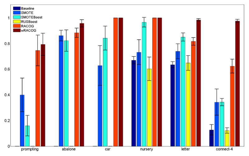
The primary limitation of classifiers that model imbalanced class datasets is in achieving desirable prediction accuracy for minority class instances. That is, the sensitivity is typically low assuming that the minority class is represented as the positive class. The proposed approaches place emphasis on boosting the sensitivity of the classifiers while maintaining a strong prediction performance for both of the classes, which is measured by G-mean. However, we understand that the choice of performance measure that needs to be boosted when dealing with class imbalanced dataset is tightly coupled with the application domain. Moreover, finding a trade-off between improving classifier performance on the minority class in isolation and on the overall dataset should ideally be left at the discretion of the domain expert.

We compare the sensitivity of this C4.5 decision tree on all six approaches in Figure 7. From the figure it is quite evident that both RACOG and wRACOG perform better than the other methods. Also, there is not too much performance variability for RACOG and wRACOG over the five cross validation. RUSBoost fails by performing nowhere close to the oversampling techniques. The poor performance of RUSBoost can be attributed to the rarity of minority class samples in the datasets under consideration. When the minority class samples are already rare, random under-sampling of majority class to achieve a 35:65 class distribution (as done by RUSBoost) at each iteration of RUSBoost, makes the majority class samples rare as well. Thus, the weak leaner of RUSBoost does not learn anything on the majority class which increases the error rate of the hypothesis at every iteration. Both SMOTE and SMOTEBoost are good contenders, although SMOTEBoost outperforms SMOTE in most of the cases. Although wRACOG performs better than RACOG on four datasets, they perform equally well for the car and nursery datasets. We verify the statistical significance of these improvements using a Student’s t test. RACOG and wRACOG do exhibit significant (p < 0.05) performance improvement over SMOTEBoost. The statistical significance of the performance improvements of RACOG and wRACOG over SMOTEBoost for alternative classifiers are reported in bold in Tables 5, 6 and 7.

Fig. 7.

Sensitivity for C4.5 Decision Tree

TABLE 5.

Results for SVM

Sensitivity
Dataset	Baseline	SMOTE	SMOTEBoost	RUSBoost	RACOG	wRACOG
prompting	0.0000 ± 0.0000	0.6667 ± 0.0667	0.2600 ± 0.0641	0.0000 ± 0.0000	0.5600 ± 0.1011	0.5400 ± 0.0723
abalone	0.0000 ± 0.0000	0.9462 ± 0.0251	0.8462 ± 0.0769	0.0000 ± 0.0000	0.9385 ± 0.0161	0.9846 ± 0.0161
car	0.0000 ± 0.0000	1.0000 ± 0.0000	0.9000 ± 0.1195	0.0000 ± 0.0000	1.0000 ± 0.0000	1.0000 ± 0.0000
nursery	0.0000 ± 0.0000	0.9939 ± 0.0136	0.9848 ± 0.0186	0.7091 ± 0.0529	1.0000 ± 0.0000	1.0000 ± 0.0000
letter	0.4645 ± 0.0430	0.9026 ± 0.0409	0.9092 ± 0.0388	0.6487 ± 0.0396	0.9289 ± 0.0220	0.9364 ± 0.0166
connect-4	0.0000 ± 0.0000	0.6233 ± 0.0473	0.5680 ± 0.0383	0.0000 ± 0.0000	0.7880 ± 0.0390	0.9867 ± 0.0153

G-mean
Dataset	Baseline	SMOTE	SMOTEBoost	RUSBoost	RACOG	wRACOG
prompting	0.0000 ± 0.0000	0.7653 ± 0.0419	0.5008 ± 0.0587	0.0000 ± 0.0000	0.7184 ± 0.0612	0.7053 ± 0.0430
abalone	0.0000 ± 0.0000	0.8049 ± 0.0079	0.8087 ± 0.0324	0.0000 ± 0.0000	0.8020 ± 0.0096	0.7850 ± 0.0140
car	0.0000 ± 0.0000	0.9629 ± 0.0028	0.9278 ± 0.0633	0.0000 ± 0.0000	0.9632 ± 0.0076	0.9660 ± 0.0075
nursery	0.0000 ± 0.0000	0.9742 ± 0.0065	0.9817 ± 0.0095	0.8403 ± 0.0320	0.9660 ± 0.0020	0.9760 ± 0.0042
letter	0.6804 ± 0.0316	0.9341 ± 0.0223	0.9484 ± 0.0195	0.8034 ± 0.0244	0.9351 ± 0.0115	0.9395 ± 0.0046
connect-4	0.0000 ± 0.0000	0.7306 ± 0.0282	0.7135 ± 0.0221	0.0000 ± 0.0000	0.8007 ± 0.0210	0.8269 ± 0.0351

AUC-ROC
Dataset	Baseline	SMOTE	SMOTEBoost	RUSBoost	RACOG	wRACOG
prompting	0.5000 ± 0.0000	0.7734 ± 0.0384	0.8620 ± 0.0170	0.5000 ± 0.0000	0.7437 ± 0.0490	0.7332 ± 0.0316
abalone	0.5000 ± 0.0000	0.8156 ± 0.0100	0.8792 ± 0.0339	0.5000 ± 0.0000	0.8121 ± 0.0074	0.8054 ± 0.0102
car	0.5000 ± 0.0000	0.9636 ± 0.0027	0.9772 ± 0.0132	0.5000 ± 0.0000	0.9639 ± 0.0073	0.9666 ± 0.0073
nursery	0.5000 ± 0.0000	0.9744 ± 0.0065	0.9958 ± 0.0006	0.8530 ± 0.0264	0.9665 ± 0.0020	0.9763 ± 0.0041
letter	0.7315 ± 0.0213	0.9348 ± 0.0214	0.9915 ± 0.0050	0.8222 ± 0.0194	0.9351 ± 0.0114	0.9396 ± 0.0045
connect-4	0.5000 ± 0.0000	0.7402 ± 0.0238	0.8503 ± 0.0081	0.5000 ± 0.0000	0.8010 ± 0.0204	0.8210 ± 0.0203

TABLE 6.

Results for k-Nearest Neighbor

Sensitivity
Dataset	Baseline	SMOTE	SMOTEBoost	RUSBoost	RACOG	wRACOG
prompting	0.0533 ± 0.0298	0.6333 ± 0.0471	0.4667 ± 0.2055	0.0600 ± 0.0435	0.7533 ± 0.0767	0.6600 ± 0.0760
abalone	0.0000 ± 0.0000	0.8885 ± 0.0498	0.8308 ± 0.0896	0.0000 ± 0.0000	0.8846 ± 0.0360	0.9423 ± 0.0136
car	0.0429 ± 0.0639	0.7571 ± 0.1644	0.9286 ± 0.0505	0.0286 ± 0.0391	1.0000 ± 0.0000	1.0000 ± 0.0000
nursery	0.3121 ± 0.0409	0.9364 ± 0.0561	0.9727 ± 0.0166	0.3303 ± 0.0046	1.0000 ± 0.0000	1.0000 ± 0.0000
letter	0.7566 ± 0.0372	0.9118 ± 0.0374	0.8987 ± 0.0253	0.7250 ± 0.0225	0.9211 ± 0.0186	0.9189 ± 0.0166
connect-4	0.0360 ± 0.0134	0.7133 ± 0.0586	0.4940 ± 0.0654	0.0380 ± 0.0110	0.6100 ± 0.0436	0.8833 ± 0.0651

G-mean
Dataset	Baseline	SMOTE	SMOTEBoost	RUSBoost	RACOG	wRACOG
prompting	0.2243 ± 0.0607	0.7547 ± 0.0268	0.6449 ± 0.1423	0.2144 ± 0.1318	0.8272 ± 0.0418	0.7798 ± 0.0405
abalone	0.0000 ± 0.0000	0.8301 ± 0.0198	0.8177 ± 0.0367	0.0000 ± 0.0000	0.8311 ± 0.0192	0.7841 ± 0.0127
car	0.1290 ± 0.1810	0.8093 ± 0.0729	0.9193 ± 0.0244	0.1069 ± 0.1464	0.8916 ± 0.0187	0.9471 ± 0.0071
nursery	0.5578 ± 0.0358	0.9262 ± 0.0206	0.9670 ± 0.0105	0.5741 ± 0.0309	0.9171 ± 0.0040	0.9832 ± 0.0025
letter	0.8683 ± 0.0213	0.9361 ± 0.0198	0.9366 ± 0.0122	0.8503 ± 0.0130	0.9350 ± 0.0102	0.9431 ± 0.0099
connect-4	0.1869 ± 0.0358	0.7097 ± 0.0295	0.6596 ± 0.0445	0.1932 ± 0.0276	0.7153 ± 0.0250	0.6911 ± 0.0184

AUC-ROC
Dataset	Baseline	SMOTE	SMOTEBoost	RUSBoost	RACOG	wRACOG
prompting	0.8707 ± 0.0225	0.8670 ± 0.0228	0.8168 ± 0.0197	0.5290 ± 0.0214	0.8854 ± 0.0307	0.8905 ± 0.0168
abalone	0.8819 ± 0.0179	0.8760 ± 0.0338	0.8783 ± 0.0243	0.5000 ± 0.0000	0.8812 ± 0.0210	0.8725 ± 0.0089
car	0.9930 ± 0.0035	0.9543 ± 0.0129	0.9724 ± 0.0112	0.5143 ± 0.0196	0.9932 ± 0.0035	0.9941 ± 0.0043
nursery	0.9999 ± 0.0003	0.9875 ± 0.0073	0.9949 ± 0.0016	0.6652 ± 0.0173	0.9994 ± 0.0002	0.9990 ± 0.0004
letter	0.9872 ± 0.0051	0.9818 ± 0.0074	0.9808 ± 0.0077	0.8613 ± 0.0110	0.9860 ± 0.0062	0.9887 ± 0.0018
connect-4	0.7744 ± 0.0426	0.7732 ± 0.0185	0.7844 ± 0.0235	0.5183 ± 0.0054	0.8262 ± 0.0241	0.7824 ± 0.0349

TABLE 7.

Results for Logistic Regression

Sensitivity
Dataset	Baseline	SMOTE	SMOTEBoost	RUSBoost	RACOG	wRACOG
prompting	0.0867 ± 0.0447	0.5667 ± 0.0850	0.2933 ± 0.1657	0.1533 ± 0.0380	0.4667 ± 0.1179	0.4867 ± 0.1043
abalone	0.0000 ± 0.0000	0.9154 ± 0.0258	0.8962 ± 0.0322	0.0000 ± 0.0000	0.8923 ± 0.0421	0.9308 ± 0.0586
car	0.3429 ± 0.1174	0.9571 ± 0.0639	0.8714 ± 0.0782	0.3286 ± 0.1481	1.0000 ± 0.0	1.0000 ± 0.0000
nursery	0.7394 ± 0.0127	0.9424 ± 0.0628	0.9515 ± 0.0392	0.7576 ± 0.0557	1.0000 ± 0.0000	1.0000 ± 0.000
letter	0.6171 ± 0.0482	0.9000 ± 0.0471	0.9197 ± 0.0086	0.6566 ± 0.0205	0.9184 ± 0.0231	0.9518 ± 0.0249
connect-4	0.2920 ± 0.0785	0.6300 ± 0.0361	0.5600 ± 0.0543	0.3040 ± 0.0439	0.8120 ± 0.0327	1.0000 ± 0.0000

G-mean
Dataset	Baseline	SMOTE	SMOTEBoost	RUSBoost	RACOG	wRACOG
prompting	0.2845 ± 0.0782	0.7186 ± 0.0503	0.5141 ± 0.1537	0.3861 ± 0.0497	0.6596 ± 0.0784	0.6722 ± 0.0778
abalone	0.0000 ± 0.0000	0.8441 ± 0.0184	0.8264 ± 0.0245	0.0000 ± 0.0000	0.8290 ± 0.0197	0.7971 ± 0.0496
car	0.5746 ± 0.0979	0.9543 ± 0.0322	0.9092 ± 0.0410	0.5556 ± 0.1362	0.9747 ± 0.0050	0.9716 ± 0.0040
nursery	0.8573 ± 0.0066	0.9600 ± 0.0309	0.9655 ± 0.0189	0.8679 ± 0.0319	0.9860 ± 0.0017	0.9887 ± 0.0013
letter	0.7826 ± 0.0305	0.9243 ± 0.0252	0.9329 ± 0.0076	0.8082 ± 0.0122	0.9270 ± 0.0114	0.9286 ± 0.0100
connect-4	0.5293 ± 0.0778	0.7383 ± 0.0234	0.7051 ± 0.0317	0.5438 ± 0.0409	0.8046 ± 0.0164	0.8142 ± 0.0451

AUC-ROC
Dataset	Baseline	SMOTE	SMOTEBoost	RUSBoost	RACOG	wRACOG
prompting	0.8714 ± 0.0173	0.8643 ± 0.0371	0.8404 ± 0.0246	0.5691 ± 0.0192	0.8269 ± 0.0482	0.8222 ± 0.0124
abalone	0.8914 ± 0.0082	0.8900 ± 0.0167	0.8756 ± 0.0191	0.4999 ± 0.2852	0.8914 ± 0.0149	0.8832 ± 0.0304
car	0.9778 ± 0.0031	0.9758 ± 0.0039	0.9652 ± 0.0054	0.6562 ± 0.0754	0.9731 ± 0.0080	0.9741 ± 0.0065
nursery	0.9954 ± 0.0007	0.9948 ± 0.0010	0.9923 ± 0.0009	0.8764 ± 0.0279	0.9956 ± 0.0007	0.9948 ± 0.0010
letter	0.9817 ± 0.0025	0.9782 ± 0.0055	0.9756 ± 0.0066	0.8258 ± 0.0096	0.9810 ± 0.0048	0.9787 ± 0.0065
connect-4	0.8769 ± 0.0086	0.8538 ± 0.0088	0.8320 ± 0.0157	0.6403 ± 0.0238	0.8742 ± 0.0276	0.8840 ± 0.0066

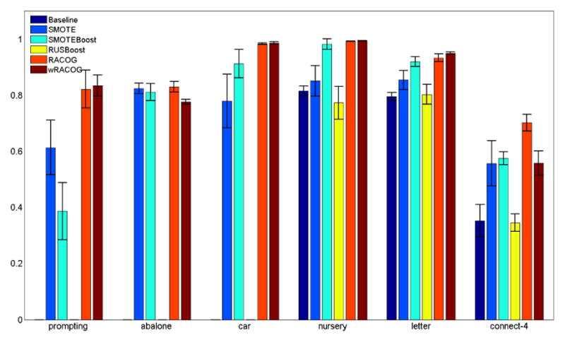
Because the sampling techniques boost the minority class, there is a tendency for the false positive rate to increase. However, the increase in false positive rate is not very significant and therefore it does not affect the G-mean scores. Figure 8 reports the G-mean scores of C4.5 decision tree on all the methods when tested with the six datasets. Clearly, RACOG and wRACOG result in a superior performance over SMOTE and SMOTEBoost. However, SMOTEBoost is a very strong contender.

Fig. 8.

G-mean for C4.5 Decision Tree

In Figure 9, we plot the ROC curves produced by the different approaches on each of the 6 datasets when evaluated with a C4.5 decision tree. For the prompting, abalone and car datasets, Baseline and RUS-Boost do not perform any better than random prediction. The performance of RACOG and wRACOG are clearly better than SMOTE and SMOTEBoost for the prompting dataset. However, there is no clear winner among them for the abalone, car and nursery datasets. The AUC-ROCs are reported in Table 4. For the letter and connect-4 datasets, the AUC-ROC for SMOTEBoost is higher than RACOG and wRACOG. However, no statistically significant improvement of RACOG and wRACOG was found over SMOTEBoost based on AUC-ROC. Also, as there is no clear winner between RACOG and wRACOG on any of the performance measures we do not conduct any statistical significance test between them.

Fig. 9.

ROC curves produced by C4.5 Decision Tree

TABLE 4.

AUC-ROC for C4.5 Decision Tree

Dataset	Baseline	SMOTE	SMOTEBoost	RUSBoost	RACOG	wRACOG
prompting	0.5000 ± 0.0000	0.8681 ± 0.0359	0.8546 ± 0.0334	0.5000 ± 0.0000	0.8851 ± 0.0207	0.8717 ± 0.0404
abalone	0.5000 ± 0.0000	0.8693 ± 0.0272	0.8718 ± 0.0262	0.5000 ± 0.0000	0.8646 ± 0.0233	0.8727 ± 0.0208
car	0.5000 ± 0.0000	0.9595 ± 0.0320	0.9957 ± 0.0025	0.5000 ± 0.0000	0.9879 ± 0.0027	0.9904 ± 0.0067
nursery	0.9849 ± 0.0077	0.9515 ± 0.0219	0.9999 ± 0.0001	0.7999 ± 0.0456	0.9968 ± 0.0005	0.9967 ± 0.0005
letter	0.8745 ± 0.0056	0.9340 ± 0.0153	0.9865 ± 0.0080	0.8226 ± 0.0286	0.9659 ± 0.0102	0.9707 ± 0.0026
connect-4	0.6215 ± 0.0310	0.6907 ± 0.0335	0.8317 ± 0.0140	0.5552 ± 0.0092	0.7333 ± 0.0181	0.7115 ± 0.0282

Convergence Diagnostic Test

In the current work we explore the strengths of Markov chain Monte Carlo techniques, specifically Gibbs sampling, to generate new minority class samples. A major issue for the successful implementation of any MCMC technique is to determine the number of iterations required for the generated samples to converge to the target distribution.

Researchers in econometrics [51] use formal methods such as the Raftery-Lewis test [49] to make this determination. Given outputs from a Gibbs sampler, the Raftery-Lewis test provides the answer to: how long to monitor the chain of samples? Here, one specifies a particular quantile q of the distribution of interest (typically 2.5% and 97.5%, to give a 95% confidence interval), an accuracy σ of the quantile, and a power 1 − β for achieving this accuracy on the specified quantile. These parameters are used to determine the burn-in (M), the total number of iterations required to achieve the desired accuracy for the posterior (N), the appropriate lag (k), and the number of iterations(N_min) that would be needed if the samples represented an independent and identically distributed (iid)⁵ chain, which is not true in our case because of the autocorrelation structure present in the Markov chain of generated samples.

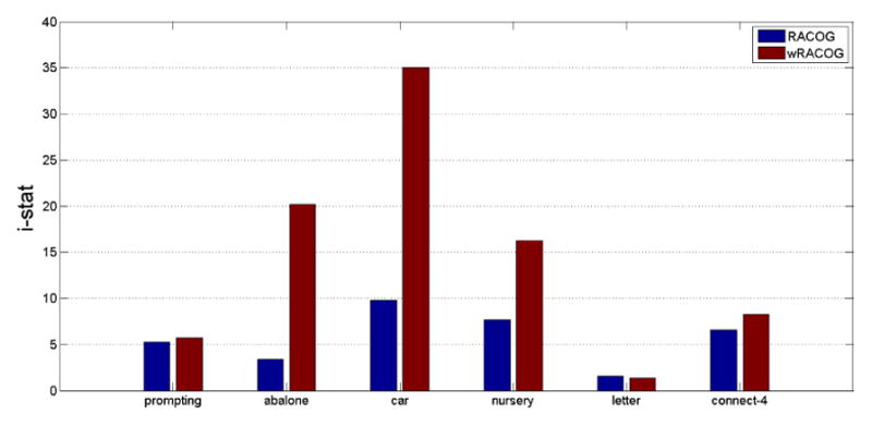
The diagnostic was designed to test the number of iterations and burn-in needed, by first running and testing a shorter pilot chain. In practice, it is also used to test any normal Markov chain generated by a Gibbs sampler to see if it satisfies the results that the diagnostic suggests. These output values can be combined to calculate i-stat defined as follows:

$$i-\mathit{stat}=\frac{M+N}{N_{\mathit{min}}}$$ (11)

i-stat measures the increase in the number of iterations due to dependence in the sequence (Markov chain). Raftery and Lewis indicate that i-stat is indicative of a convergence of the sampler if the value does not exceed 5.

From Figure 10 it is evident that convergence is almost achieved by both RACOG and wRACOG for the prompting and letter datasets. However, the wRACOG i-stat value is greater than the RACOG value for the remainder of the datasets. Although this indicates that wRACOG could not converge to the target minority class distribution for the abalone, nursery and car datasets, we have seen that the wRACOG sensitivity and G-mean are better or at par with RACOG. Therefore, one explanation is that convergence here (not necessarily probabilistic) is subjective as it is tightly coupled with the application.

Fig. 10.

i-stat values for RACOG and wRACOG

We further analyze the convergence of RACOG and wRACOG in terms of the number of iterations the Gibbs sampler undergoes to achieve the i-stat value reported in Figure 10. From Figure 11 we notice that wRACOG generates a much fewer (except for connect-4 dataset) number of iterations (~ 63%) than RACOG. This explains the poor performance of wRACOG in terms of probabilistic convergence on the Raftery-Lewis test. However, the sensitivity and G-mean score are not affected by the reduction in the number of iterations.

Fig. 11.

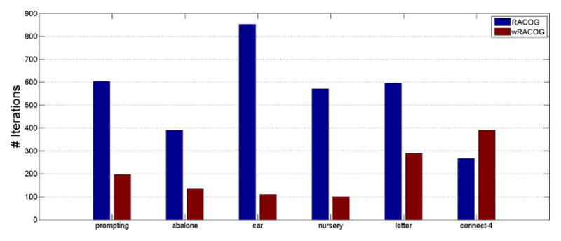
Comparison of total number of iterations required by different methods to achieve given i-stat

The number of samples added to the baseline datasets by the different oversampling algorithms for achieving the reported performance is also an important parameter to analyze. Ideally, we would want to obtain a high performance by adding as less number of samples as possible. Figure 12 illustrates the number of samples added by the different approaches. As the number of samples added by SMOTEBoost is far higher than other methods, we present log₁₀ values of the number of added samples so that the comparison could be better represented in the plot. SMOTE and RACOG try to achieve a 50:50 class distribution and thus add samples accordingly. SMOTEBoost requires ten boosting iterations to produce ten hypotheses on which weighted voting is performed while prediction. The hypothesis learned at each iteration of SMOTE-Boost has the form: h_t : X × Y → [0, 1], and therefore stores the instances generated by SMOTE at every iteration. Hence, SMOTEBoost adds ten times the number of samples added by SMOTE. On the other hand, wRACOG requires a fraction (~ 56%) of the number of samples generated by SMOTE and RACOG, and (~ 5.6%) of the number of samples generated by SMOTEBoost, to obtain superior performance. We attribute this behavior to wRACOG’s sample selection methodology which ensures the diversity in the samples that are added.

Fig. 12.

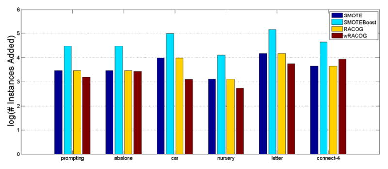
Comparison of log(number of instances added) by different methods

7 Conclusion

In this paper, we propose two Gibbs sampling-based algorithms for generating new minority class samples for class imbalanced datasets. While conventional Gibbs sampling uses joint probability distribution of data attributes to generate samples, we do not find this approach to be suitable for class imbalanced datasets which (mostly) contains rare minority class samples. As a solution, we use a Bayesian tree-based approach to impose dependencies among attributes. Both the proposed approaches, RACOG and wRACOG, use Gibbs sampling at their core. However, they differ in the sample selection strategy. RACOG runs the Gibbs sampler for a predetermined number of iterations and selects samples from the Markov chain generated by the Gibbs sampler using predefined burn-in and lag. On the other hand, wRACOG selects samples that have the highest probability of being misclassified by the existing learning model. It keeps on adding samples unless there is no further improvement in sensitivity over a predefined number of most recent iterations.

Experiments with RACOG and wRACOG on a wide variety of datasets and classifiers indicate that the algorithm is able to attain higher sensitivity than other methods, while maintaining higher G-mean. This supports our hypotheses that generating new samples by considering the global distribution of minority class points is a good approach for dealing with class imbalance. The motivation to focus mainly on improving sensitivity comes from the our application domain in pervasive computing. However, we ensure that the performance of the classifiers on both the classes is not hampered.

In the future, we want to experiment with alternative methods to the Bayesian tree to see if attribute dependencies could be captured more accurately. As the current Bayesian tree approach is computationally lightweight, we would ensure that this property is preserved while experimenting with alternative approaches. Also, we would propose RACOGBoost by combining the advantages of boosting with that of RACOG.

Biographies

Barnan Das is a PhD candidate in Computer Science at Washington State University. He received his Bachelor of Technology degree in Computer Science and Engineering from West Bengal University of Technology, Kolkata, India in 2009. His research interests include machine learning, data mining, artificial intelligence and smart environments. Including IEEE, Mr. Das is also Student Member with ACM SIGKDD and SIAM.

Narayanan C. Krishnan completed his PhD in Computer Science in December 2010 from Arizona State University. He is currently working as Assistant Research Professor at Washington State University. Narayanan received his Bachelors and Masters in Science majoring in Mathematics from Sri Sathya Sai Institute of Higher Learning in 2000 and 2002 respectively. He then went on to complete his Masters in Technology (Computer Science) also from the same university in 2004. His research interests are in the area of activity recognition, pattern recognition and machine learning for pervasive computing applications

Diane J. Cook is a Huie-Rogers Chair Professor in the School of Electrical Engineering and Computer Science at Washington State Univeristy. Dr. Cook received a B.S. degree in Math/Computer Science from Wheaton College in 1985, a M.S. degree in Computer Science from the University of Illinois in 1987, and a Ph.D. degree in Computer Science from the University of Illinois in 1990. Her research interests include artificial intelligence, machine learning, graph-based relational data mining, smart environments, and robotics. Dr. Cook is an IEEE Fellow.

References

- 1.Woods K, Doss C, Bowyer K, Solka J, Priebe C, KW Comparative evaluation of pattern recognition techniques for detection of microcalcifications in mammography. International Journal of Pattern Recognition and Artificial Intelligence. 1993;7(6):1417–1436. [Google Scholar]
- 2.Kubat M, Holte R, Matwin S. Machine learning for the detection of oil spills in satellite radar images. Machine learning. 1998;30(2):195–215. [Google Scholar]
- 3.Phua C, Alahakoon D, Lee V. Minority report in fraud detection: classification of skewed data. ACM SIGKDD Explorations Newsletter. 2004;6(1):50–59. [Google Scholar]
- 4.Turney P, et al. Learning algorithms for keyphrase extraction. Information Retrieval. 2000;2(4):303–336. [Google Scholar]
- 5.Lewis D, Gale W. A sequential algorithm for training text classifiers. Proceedings of the 17th Annual International ACM SIGIR Conference on Research and Development in Information Retrieval; Springer-Verlag New York, Inc; 1994. pp. 3–12. [Google Scholar]
- 6.Liu A, Ghosh J, Martin C. Generative oversampling for mining imbalanced datasets. Proceedings of the 2007 International Conference on Data Mining, DMIN; 2007; pp. 25–28. [Google Scholar]
- 7.Zadrozny B, Langford J, Abe N. Cost-sensitive learning by cost-proportionate example weighting. Third IEEE International Conference on Data Mining, 2003. ICDM 2003; IEEE; 2003. pp. 435–442. [Google Scholar]
- 8.Elkan C. International Joint Conference on Artificial Intelligence. 1. Vol. 17. Lawrence Erlbaum Associates Ltd; 2001. The foundations of cost-sensitive learning; pp. 973–978. [Google Scholar]
- 9.McCarthy K, Zabar B, Weiss G. Does cost-sensitive learning beat sampling for classifying rare classes?. Proceedings of the 1st international workshop on Utility-based data mining; ACM; 2005. pp. 69–77. [Google Scholar]
- 10.Maloof M. Learning when data sets are imbalanced and when costs are unequal and unknown. ICML-2003 Workshop on Learning from Imbalanced Data Sets II; 2003. [Google Scholar]
- 11.Weiss G. Mining with rarity: a unifying framework. SigKDD Explorations. 2004;6(1):7–19. [Google Scholar]
- 12.Seiffert C, Khoshgoftaar T, Van Hulse J, Napolitano A. RUSBoost: A hybrid approach to alleviating class imbalance. Systems Man and Cybernetics Part A: Systems and Humans IEEE Transactions on. 2010;40(1):185–197. [Google Scholar]
- 13.Chawla N, Bowyer K, Hall L, Kegelmeyer W. SMOTE: synthetic minority over-sampling technique. Journal of Artificial Intelligence Research. 2002 Jun;16:321–357. [Google Scholar]
- 14.Chawla N, Lazarevic A, Hall L, Bowyer K. SMOTE-Boost: Improving prediction of the minority class in boosting. Knowledge Discovery in Databases: PKDD 2003. 2003:107–119. [Google Scholar]
- 15.Chawla N, Japkowicz N, Kotcz A. Editorial: special issue on learning from imbalanced data sets. ACM SIGKDD Explorations Newsletter. 2004;6(1):1–6. [Google Scholar]
- 16.He H, Garcia E. Learning from imbalanced data. IEEE Transactions on Knowledge and Data Engineering. 2009;21(9):1263–1284. [Google Scholar]
- 17.Sun Y, Wong A, Kamel M. Classification of imbalanced data: A review. International Journal of Pattern Recognition and Artificial Intelligence. 2009;23(4):687. [Google Scholar]
- 18.Chawla N. Data mining for imbalanced datasets: An overview. Data Mining and Knowledge Discovery Handbook. 2010:875–886. [Google Scholar]
- 19.Liu X, Zhou Z. The influence of class imbalance on cost-sensitive learning: an empirical study. Data Mining, 2006. ICDM’06. Sixth International Conference on; IEEE; 2006. pp. 970–974. [Google Scholar]
- 20.Weiss G, McCarthy K, Zabar B. Cost-sensitive learning vs. sampling: Which is best for handling unbalanced classes with unequal error costs. International Conference on Data Mining; 2007; pp. 35–41. [Google Scholar]
- 21.Provost F, Fawcett T, Kohavi R. The case against accuracy estimation for comparing induction algorithms. Proceedings of the Fifteenth International Conference on Machine Learning; 1998. [Google Scholar]
- 22.Drummond C, Holte R. Exploiting the cost (in) sensitivity of decision tree splitting criteria. Machine Learning-International Workshop then Conference; 2000; pp. 239–246. [Google Scholar]
- 23.Kukar M, Kononenko I. Cost-sensitive learning with neural networks. Proceedings of the 13th European Conference on Artificial Intelligence (ECAI-98); Citeseer. 1998; pp. 445–449. [Google Scholar]
- 24.Hong X, Chen S, Harris C. A kernel-based two-class classifier for imbalanced data sets. IEEE Transactions on Neural Networks. 2007;18(1):28–41. doi: 10.1109/TNN.2006.882812. [DOI] [PubMed] [Google Scholar]
- 25.Wu G, Chang E. Kba: Kernel boundary alignment considering imbalanced data distribution. IEEE Transactions on Knowledge and Data Engineering. 2005;17(6):786–795. [Google Scholar]
- 26.Fung G, Mangasarian O. Multicategory proximal support vector machine classifiers. Machine Learning. 2005;59(1):77–97. [Google Scholar]
- 27.Han H, Wang W, Mao B. Borderline-SMOTE: A new over-sampling method in imbalanced data sets learning. Advances in Intelligent Computing. 2005:878–887. [Google Scholar]
- 28.He H, Bai Y, Garcia E, Li S. ADASYN: Adaptive synthetic sampling approach for imbalanced learning. IEEE International Joint Conference on Neural Networks, 2008 (IEEE World Congress on Computational Intelligence); IEEE; 2008. pp. 1322–1328. [Google Scholar]
- 29.Jo T, Japkowicz N. Class imbalances versus small disjuncts. ACM SIGKDD Explorations Newsletter. 2004;6(1):40–49. [Google Scholar]
- 30.Liu X, Wu J, Zhou Z. Exploratory undersampling for class-imbalance learning. Systems Man and Cybernetics Part B: Cybernetics, IEEE Transactions on. 2009;39(2):539–550. doi: 10.1109/TSMCB.2008.2007853. [DOI] [PubMed] [Google Scholar]
- 31.García V, Mollineda R, Sánchez J. On the k-nn performance in a challenging scenario of imbalance and overlapping. Pattern Analysis & Applications. 2008;11(3):269–280. [Google Scholar]
- 32.Tomek I. Two modifications of cnn. IEEE Transaction on Systems, Man and Cybernetics. 1976;6:769–772. [Google Scholar]
- 33.Kubat M, Matwin S. Machine Learning-International Workshop then Conference. Morgan Kaufmann Publishers, Inc; 1997. Addressing the curse of imbalanced training sets: one-sided selection; pp. 179–186. [Google Scholar]
- 34.Batista G, Prati R, Monard M. A study of the behavior of several methods for balancing machine learning training data. ACM SIGKDD Explorations Newsletter. 2004;6(1):20–29. [Google Scholar]
- 35.Galar M, Fernández A, Barrenechea E, Bustince H, Herrera F. A review on ensembles for the class imbalance problem: Bagging-, boosting-, and hybrid-based approaches. IEEE Transactions on Systems Man and Cybernetics-Part : Applications and Reviews. 2012 Jul;42(4):463–484. [Google Scholar]
- 36.Błaszczyński J, Deckert M, Stefanowski J, Wilk S. Rough Sets and Current Trends in Computing. Springer; 2010. Integrating selective pre-processing of imbalanced data with ivotes ensemble; pp. 148–157. [Google Scholar]
- 37.Wang S, Yao X. Diversity analysis on imbalanced data sets by using ensemble models. Computational Intelligence and Data Mining, 2009. CIDM’09. IEEE Symposium on; IEEE; 2009. pp. 324–331. [Google Scholar]
- 38.Cook D, Schmitter-Edgecombe M, et al. Assessing the quality of activities in a smart environment. Methods of Information in Medicine. 2010;48(5):480. doi: 10.3414/ME0592. [DOI] [PMC free article] [PubMed] [Google Scholar]
- 39.Doctor F, Hagras H, Callaghan V. A fuzzy embedded agent-based approach for realizing ambient intelligence in intelligent inhabited environments. IEEE Transactions on Systems Man and Cybernetics Part A: Systems and Humans. 2005;35(1):55–65. [Google Scholar]
- 40.Lawton M, Nahemow L. In: Environment and aging theory: A focus on aging. Scheidt R, Windley P, editors. Greenwood Press; 1998. [Google Scholar]
- 41.Mihailidis A, Fernie G, Barbenel J. The use of artificial intelligence in the design of an intelligent cognitive orthosis for people with dementia. Assistive Technology. 2001;13(1):23–39. doi: 10.1080/10400435.2001.10132031. [DOI] [PubMed] [Google Scholar]
- 42.Seelye AM, Das S-EMB, Cook DJ. Using cognitive rehabilitation theory to inform the development of smart prompting technologies. Reviews in Biomedical Engineering. 2012 doi: 10.1109/RBME.2012.2196691. to appear. [DOI] [PMC free article] [PubMed] [Google Scholar]
- 43.Meteopolis N, Ulam S. The monte carlo method. Journal of the American statistical association. 1949;44(247):335–341. doi: 10.1080/01621459.1949.10483310. [DOI] [PubMed] [Google Scholar]
- 44.Metropolis N, Rosenbluth A, Rosenbluth M, Teller A, Teller E. Equation of state calculations by fast computing machines. The Journal of Chemical Physics. 1953;21:1087. [Google Scholar]
- 45.Geyer C. Practical markov chain monte carlo. Statistical Science. 1992;7(4):473–483. [Google Scholar]
- 46.Friedman N, Geiger D, Goldszmidt M. Bayesian network classifiers. Machine learning. 1997;29(2):131–163. [Google Scholar]
- 47.Weiss G, Provost F. Learning when training data are costly: The effect of class distribution on tree induction. Journal of Artificial Intelligence Research (JAIR) 2003;19:315–354. [Google Scholar]
- 48.Khoshgoftaar T, Seiffert C, Van Hulse J, Napolitano A, Folleco A. Learning with limited minority class data. Machine Learning and Applications, 2007. ICMLA 2007. Sixth International Conference on; IEEE; 2007. pp. 348–353. [Google Scholar]
- 49.Raftery A, Lewis S. How many iterations in the gibbs sampler. Bayesian statistics. 1992;4(2):763–773. [Google Scholar]
- 50.Huang J, Ling C. Using auc and accuracy in evaluating learning algorithms. IEEE Transactions on Knowledge and Data Engineering. 2005;17(3):299–310. [Google Scholar]
- 51.LeSage J, Pace R. Introduction to spatial econometrics. Vol. 196 Chapman & Hall/CRC; 2009. [Google Scholar]