Abstract
We present the software CDpal that is used to analyze thermal and chemical denaturation data to obtain information on protein stability. The software uses standard assumptions and equations applied to two‐state and various types of three‐state denaturation models in order to determine thermodynamic parameters. It can analyze denaturation monitored by both circular dichroism and fluorescence spectroscopy and is extremely flexible in terms of input format. Furthermore, it is intuitive and easy to use because of the graphical user interface and extensive documentation. As illustrated by the examples herein, CDpal should be a valuable tool for analysis of protein stability.
Keywords: protein stability, thermal denaturation, chemical denaturation, circular dichroism, fluorescence, curve fitting, protein stability software, protein denaturation software
Introduction
Analysis of stability is important in biophysical characterization of proteins and involves determination of differences in thermodynamic parameters between the native and denatured states. Stability can however have several definitions and may for instance be defined as stability against changes in temperature or against presence of chaotropic agents. To determine these parameters one employs a method that gives distinct signals for the native and denatured states.
A common method for assaying thermal stability is to use circular dichroism (CD) spectroscopy and monitor the temperature dependence of the signal at a fixed wavelength. In the classic work by Greenfield and Fasman, 222 and 217 nm were reported as CD signal extremums for α‐helices and β‐strands,1 respectively, and consequently these wavelengths are good choices. For the analysis of chemical stability, fluorescence spectroscopy, where the change in environment of tryptophan residues commonly is used as a proxy for denaturation, is often the method of choice. The CD or fluorescence signal for a protein is the population weighted sum of the signals for all states present and since populations can be calculated from equilibrium constants it follows that thermodynamic parameters can be determined by fits of CD or fluorescence profiles as functions of temperature or denaturant concentration.
In addition to software developed by the manufacturers of spectrometers there are graphical packages that can be used to evaluate protein stability data. Examples include:
GraphPad (http://www.graphpad.com), Psi‐Plot (http://www.polysoftware.com/aboutpsi.htm), Origin (http://www.originlab.com), and SigmaPlot (http://www.systat.com). Despite this, analysis of protein stability is often oversimplified and frequently done without proper fitting. The reason for this may be that existing applications are not versatile enough or sufficiently user‐friendly. Our software CDpal is intended to fill this gap. The primary aim of the software was fast, accurate and versatile curve fitting in a user‐friendly environment. Thus, curve fitting of thermal or chemical stability data and interpretation of the results are straightforward and aided by a detailed help section. The fits are shown graphically and images as well as thermodynamic parameters can be exported. CDpal can fit data to the standard two‐state model but also to models involving intermediate states. CDpal was developed with Qt 5.4.1 (http://www.qt.io) together with the Qt C++ widget QCustomPlot (Emanuel Eichhammer, http://www.qcustomplot.com) for Linux, OS X and Windows.
The fitting in CDpal is based on the two main assumptions that measurements are performed at thermal equilibrium and that the signal for a particular state is a linear function of temperature or concentration of denaturant. In the following we use the denotations N and D for native and denatured protein states, respectively, and I for intermediate states. The four different models for protein denaturation described in Figure 1 and explained below are implemented in CDpal.
Figure 1.
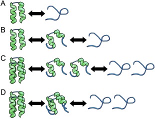
Illustration of different models for protein denaturation. (A) Denaturation is described as a two‐state, , process. (B) Unfolding proceeds via an intermediate state, . (C, D) Denaturation of a dimer where the intermediate state consists of partially denatured monomers, , or a partially denatured dimer, , respectively.
For two‐state denaturation, with equilibrium constant K, the second assumption implies
| (1) |
where f N and f D are the fractional populations of the two states, ξ is temperature or concentration of denaturant and is the signal for state i at temperature or concentration of denaturant ξ. The equilibrium constant is given by:
| (2) |
where ΔG 0, ΔH 0, and ΔS 0 are the standard changes in free energy, enthalpy, and entropy, respectively, T is the temperature and R is the universal gas constant. Provided that the difference in heat capacity, ΔC p, between the two states is independent of temperature, an alternative way of writing the equilibrium constant is:
| (3) |
where ΔH m is the change in enthalpy at the denaturation midpoint, T m, and is often referred to as the van't Hoff enthalpy. ΔH m, ΔC p, and T m can be used to calculate ΔH and ΔS at arbitrary temperatures if desired. Similarly, if the difference in free energy between the two states depends linearly on the concentration of denaturant, the equilibration constant at denaturant concentration C is
| (4) |
where C m is the denaturant concentration at the denaturation midpoint and m is the rate of change in free energy difference, which is assumed to be constant. If m and C m are known it is trivial to calculate the free energy difference between the native and denatured states in the absence of denaturants, ΔG H2O. The fractional populations of the two states are trivially
| (5a) |
| (5b) |
If denaturation proceeds via a stable intermediate I according to the scheme , with equilibrium constants K I and K D, the fractions of the three states are given by:
| (6a) |
| (6b) |
| (6c) |
For homodimers where denaturation also may proceed as or we get:
| (7a) |
| (7b) |
| (7c) |
where P 0 is the protein concentration (moles of monomers per unit volume) for the first case.2 The second case yields2
| (8a) |
| (8b) |
| (8c) |
In all these cases, the measured signal is written in full analogy with Eq. (1).
The Levenberg–Marquardt method3, 4 is used for optimization of the model parameters. This algorithm smoothly varies between the steepest descent method (far from minimum) and the inverse Hessian method (close to minimum) to update the parameters until convergence. Since there is no guarantee that the algorithm converges to the global minimum it must be supplemented with a suitable method for providing starting parameters. To estimate errors in the parameters we use the robust jackknife method.5
Results
Opening and displaying data
When CDpal is launched, the application automatically searches for newer versions online and notifies the user of available updates. After the user has selected thermal or chemical denaturation mode, the main user interface appears (Figure 2). It consists of a toolbar with the most common functions, a plot area for displaying graphs, a widget containing a table for data points and results for the data fitting and a widget for selecting which model to fit data to.
Figure 2.
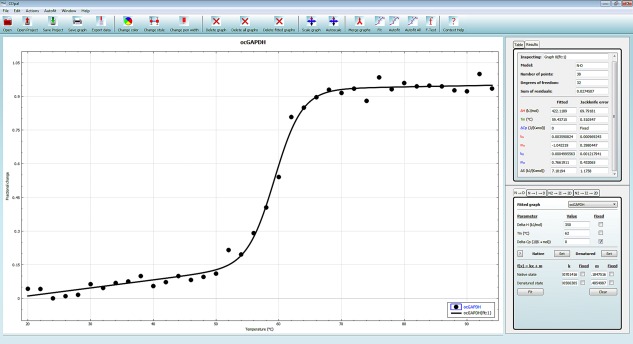
The main user interface of CDpal. The most common functions can be accessed from the toolbar at the top of the window. Input data and fitted curves are displayed in the interactive plot area where the appearance of graphs, titles, axes, and legends may be modified. Top right there is a widget containing a tab used for inspecting and selecting data points from a table and a tab for viewing results of curve fits. The lower right widget is the curve fitting interface, with separate tabs for the implemented denaturation models. Here, the user can enter initial estimates for the model parameters if automated fitting fails and can also fix certain parameters at these values rather than to optimize them.
Import of data in text format is performed by clicking Open, which brings up a file browser. If several files are selected, all are opened at once. At present only data in text format can be imported. To emphasize this and to avoid confusion, the extension. txt is required for data files. Since the format of such files differs among manufacturers of spectrometers and may even vary for different versions from the same manufacturer, CDpal allows the user to specify custom formats that can be saved as presets. The custom file format allows the user to specify which columns that correspond to temperature or concentration of denaturant and signal, respectively. It is also possible to select the number of header lines to skip or to scan the input file for a certain keyword that signals the start of the data section. The custom format is displayed as a template to clarify how data is imported. Data will be imported until end‐of‐file, a line of incorrect format is encountered or the values for temperature or concentration of denaturant start to decrease. The user can choose to normalize the signal to values between zero and one for each individual data set. After import, the data sets are immediately displayed graphically in the plot area. If desired, the user may change symbols, colors, and size of data points for a selected data set. The titles of the plot, axes, and legend items can also be changed by double clicking them. It is also possible to delete anomalous data points before fitting data. At any time, the state of a project can be saved by Save Project and the session can be reconvened at a later time point by Open Project. This is useful for adding additional data sets to an existing project.
Fitting procedure
The user must first choose which model to fit data to and usually the two‐state is adequate. To simplify the fitting procedure, CDpal includes an automated mode that is very robust for the two‐state model. By clicking Autofit or Autofit All an attempt to automatically estimate good start parameters followed by fitting the selected data set or all data sets, respectively, is performed. For thermal denaturation, the data is then fitted to a model where ΔH m and T m are optimized while ΔC p is fixed to zero. For chemical stability data the same procedure fits m and C m. If the fit converges, the fitted curve is displayed in the plot area and the fitted parameters and their associated uncertainties are shown in the result tab.
In the unlikely event of no convergence, fitting can be repeated using manually entered initial estimates. The temperature or denaturant concentration midpoint is often easy to estimate by eye and an approximate ΔH m can be estimated from protein size.6 We recommend not optimizing ΔC p but fixing it by checking the Fixed box after entering its value. For chemical denaturation, m typically ranges from 2 to 30 kJ mol−1 M−1 for GdHCl and is a factor two to three lower for urea.7 Slopes and intercepts of the native, intermediate, and denatured regions can be estimated by performing linear regression for a selected region of a data set. Clicking Fit, fits the data using manually entered starting estimates. If no combination of start parameters gives a satisfactory fit, one of the more complex models can be used in a similar fashion. If two models appear to fit the data well, F‐tests can be performed to choose the appropriate model.
Exporting the results
All results from CDpal can be exported. The graphs representing experimental data and fitted curves can be saved as publication quality images in TIFF format or images of lower quality but with smaller file sizes in JPEG or PNG format by using Save graph. The aspect ratio of the images can be modified by simply adjusting the size of the window before exporting the graphs. If the user prefers a different plotting program, e.g., with PostScript functionality, it is possible to export the data sets and fitted curves as text files with Export data. Also the model parameters may be saved to a text file.
Performance
There is no fixed upper limit on the amount of data that can be analyzed simultaneously. However, as the graphical user interface gets cramped at a certain point and visual clutter limits the clarity of graphs, it is rarely useful to analyze more than ten data sets at once. Time is generally not an issue since automated curve fitting of several data sets with satisfactory results usually is perceived as instantaneous. Indeed, an entire session in CDpal, from opening the data to exporting the results, is typically conducted in minutes or less.
In our experience automated fitting is very robust for the N⇄D model and for routine applications, there is seldom anything gained from manually providing initial values for the parameters. Automated fitting can also be attempted for the N⇄I⇄D model but likelihood of success is lower. For the models describing denaturation of dimers, automated fitting is not implemented.
The performance of CDpal has been tested for a variety of thermal and chemical denaturation data and a few representative examples are presented below. The examples are chosen to illustrate important applications, principles, difficulties, and limitations, rather than to provide textbook examples of ideal denaturation profiles.
The first example shows a typical application, the comparison of the stability for the same protein from different species. In this case, thermal stability of glyceraldehyde 3‐phosphate dehydrogenase (GAPDH) from Formica exsecta (narrow‐headed ant) and Oryctolagus cuniculis (European rabbit) was compared. From Figure 3, it is clear that the stabilities differ greatly and accordingly the fitted T m is 11.0°C larger for feGAPDH than for ocGAPDH. Despite the fact that the proteins are homotetramers, the data could be well fitted to an apparent two‐state process, which is in line with our experience that it rarely is needed to invoke the more complex models.
Figure 3.
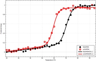
Thermal stability of GAPDH from Formica exsecta (black) and Oryctolagus cuniculis (red). The lines represent the best fit to a two‐state model with ΔC p fixed to zero. The thermodynamic parameters are T m = 70.4 ± 0.4°C, ΔH m = 390 ± 40 kJ mol−1 and T m = 59.4 ± 0.5°C, ΔH m = 420 ± 70 kJ mol−1, respectively. The image was exported from CDpal.
Our next example concerns comparison of stability between apo and ligand bound forms of the same protein, here, apo and calcium bound forms of the N‐terminal lobe of the regulatory domain of calcium dependent protein kinase 3 (CDPK3) from Plasmodium falciparum (malaria parasite).8 As can be seen in Figure 4, the profiles are quite different and while a precise estimate of T m is possible for the apo form, this is not the case for the calcium bound form and the complete absence of a post‐transition baseline makes it hard to gauge whether the automatically fitted T m = 90 ± 3°C is reliable. Indeed, this value changes significantly for other choices of starting parameters and yet the appearance of such fitted curves is essentially the same.
Figure 4.
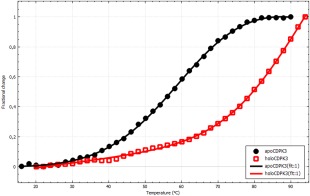
Thermal stability of apo (black) and calcium loaded (red) N‐terminal lobe of the regulatory domain of CDPK3 from Plasmodium falciparum. The data was fitted to a two‐state model with ΔC p fixed to zero. The midpoint temperature and change in enthalpy were determined to T m = 64.4 ± 0.4°C and ΔH m = 82 ± 2 kJ mol−1 and T m = 90 ± 3°C and ΔH m = 95 ± 6 kJ mol−1 for the apo and holo forms, respectively. The image was exported from CDpal.
Another common application is analysis of the stability of variants of a polymorphous protein, in this case, two variants of thiopurine methyltransferase (TMPT),9 TPMT*1 and TPMT*3C. TPMT is a marginally stable protein and various mutations have been shown to reduce stability even further.10 Additionally, the protein aggregates irreversibly at high temperature, violating the assumption of equilibrium denaturation. This is the reason for the declining post‐transition baseline in Figure 5. Since the study concerns similar systems we argue that the relative stabilities still can be compared and the conclusion is that the mutation TPMT*3C decreases T m by 8°C.
Figure 5.
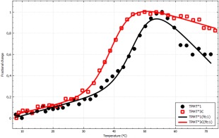
Thermal stability of human TPMT*1 (black) and TPMT*3C (red). The data was fitted to a two‐state model where ΔC p was fixed to zero. The thermodynamic parameters are T m = 47.7 ± 0.9°C, ΔH m = 250 ± 30 kJ mol−1 and T m = 39.6 ± 0.3°C, ΔH m is, 230 ± 20 kJ mol−1, respectively. The image was exported from CDpal.
The stability of the proteins in our previous examples could be well‐fitted to a two‐state process. This is not the case for the example presented in Figure 5, which is analysis of thermal stability of fatty acid binding protein (FABP)11 from Cataglyphis fortis (Saharan desert ant). Although the fit converges when the N⇄D model is used, the fitted line does obviously not connect to the data points whereas the fit looks very reasonable for the N⇄I⇄D model (Figure 6). We used the F‐test tool in CDpal to reject the two‐state model at a significance level of p = 4.72 × 10⁻¹⁸.
Figure 6.
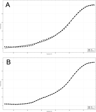
Thermal stability of C. fortis FABP fitted to (A) a two‐state process and (B) a three‐state process. ΔC p for all transitions was fixed to zero. The fitted thermodynamic parameters for the two‐state model are T m = 69.1 ± 0.4°C and ΔH m = 160 ± 10 kJ mol−1. For the three‐state model they are = 44.4 ± 0.4°C, = 66.7 ± 0.2°C, = 250 ± 40 kJ mol−1 and = 237 ± 5 kJ mol−1 for the three‐state model. The image was exported from CDpal.
We have also applied CDpal to analysis of chemical stability as exemplified in Figure 7. Here, bovine serum albumin (BSA) was subjected to increasing concentrations of urea or GdmCl and the tryptophan fluorescence at 350 nm was measured. As anticipated, higher concentrations of urea than GdmCl are required for unfolding with C m equal to 2.00 ± 0.05 and 1.41 ± 0.01M, respectively. The calculated difference in free energy, ΔG H20, are 40 ± 11 and 39 ± 7 kJ mol−1 for the experiments involving urea and GdmCl, respectively.
Figure 7.
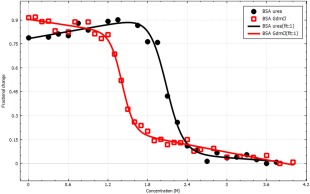
Chemical stability of BSA by urea (black) and GdmCl (red) monitored by tryptophan fluorescence at 350 nm. The fitted lines correspond to a two‐state model with thermodynamic parameters C m = 2.00 ± 0.05 M, m = 19 ± 4 kJ mol−1 M−1 and C m = 1.41 ± 0.01 M, m = 27 ± 5 kJ mol−1 M−1 for urea and GdmCl, respectively. The image was exported from CDpal.
Discussion
Since CDpal uses the same equations and models for denaturation as existing software, usage of CDpal will not result in more accurate estimates of parameters related to protein stability. The main advantages of CDpal are rather versatility and ease of use. Thermal as well as chemical denaturation can be analyzed and any method that produces a population weighted averaged signal can be used to acquire the data. Accordingly, the format of input data is not limited to that of a particular manufacturer of spectrometers and often no data conversion is necessary. Several data sets can be imported and analyzed simultaneously. In addition to the usual two‐state model for denaturation, several three‐state models are implemented. For the simpler models fitting is typically performed by a single click of the mouse. A goal when designing the software has been to make it self‐contained. It is thus for instance not necessary to trim the data from anomalous data points before import and no auxiliary programs are needed to export graphs as images in JPEG, PNG, or TIFF format. The user‐friendliness and versatility is illustrated by the examples herein.
Although not unique to CDpal, we would like to discuss some concerns when analyzing protein stability. The equations used for fitting data in CDpal and similar software are based on the assumption that measurements are performed at thermal equilibrium. To achieve equilibration for chemical denaturation it is common to prepare the samples on the day before measurements. Provided that the time constant for unfolding is on that order this is achieved but it is not uncommon with slower rates12 so that the assumption is violated. For thermal denaturation the sample is typically placed in the CD spectrometer and the temperature is raised in 1°C degree increments. Especially at the lower temperatures, the minute or so that is reserved for equilibration at each temperature is likely far from adequate. It is thus remarkable that denaturation nevertheless often is well‐fitted by CDpal and similar software. However, one of the main assumptions often is violated it is important to not overinterpret the results. In particular one should be careful when comparing data for different systems or data that have been acquired in different ways and it is useful to treat transition midpoints and differences in free energy or enthalpy as ‘apparent’ quantities that not necessarily can be reproduced in a different experimental setting. It is for this reason that we prefer to set ΔC p = 0 kJ K−1 mol−1 since even the correct value does not allow determination of the true value of ΔH m if the equilibrium condition is violated.
Another common situation that also violates the equilibrium assumption is that the denatured state aggregates irreversibly, N⇄D→A, where A is the aggregated state. A common signature of aggregation is that the CD signal for the denatured state is decreasing with increasing temperature. A sufficient condition for reversibility on the other hand is that the signal of the native state can be recovered and when denaturation is complete, the CD signal should always be monitored while the temperature is lowered to its initial value.13 Aggregation may for instance occur through a Lumry–Eyring mechanism14 where the rate constant for aggregation is temperature dependent. Although CDpal is not designed to handle this denaturation model, simulations have established that meaningful parameters still can be recovered provided that the temperature for which the rate of aggregation becomes important is sufficiently above T m. Even if this is not the case, data for similar systems can be fitted to check for differences in stability as we have done in Figure 5. In fact, by comparing the post‐transition baselines in the figure, it can also be seen that irreversible aggregation is more severe for TPMT*1 than for TPMT*3C. The pretransition baselines often have positive slopes also for reversible denaturation. We have chosen not to interpret this slope but it must obviously correspond to a gradual change of structure with temperature and we note in passing that it is possible to fit such profiles to a three‐state model with a very low value of ΔH m for the N⇄I transition while keeping the slopes of the N and I states fixed to zero.
Even if measurements of thermal stability are performed at equilibrium the data is rarely of sufficient quality to determine all three parameters at the same time. Typically, ΔC p is obtained by other means and kept fixed while and T m and ΔH m are optimized. ΔC p correlates with change in accessible surface upon unfolding and thus with protein size. The equation (units: J K−1 mol−1), where N is the number of amino acid residues has been suggested.15 It can also be determined as by measuring ΔH m and T m at multiple values of pH or from differential scanning calorimetry.16, 17
For chemical denaturation an additional assumption that may be violated is that m is independent of denaturant concentration. There are theoretical motivations for linearity7, 18 but there have also been reports on nonlinearity. In a study involving barnase, is underestimated by 15% if nonlinearity is not taken into account.19 We have however chosen to keep m constant since this is the standard treatment and since data rarely is of sufficient quality to detect deviations.
In all our examples, T m and C m are more precisely determined than ΔH m and m. If the equations are examined this is not unexpected since ΔH m and m mainly are determined by the transition region that often only contains a few data points. The close agreement of obtained for denaturation of BSA with urea and GdmCl presented in Figure 7 are therefore likely due to chance. If higher precision in ΔH m or m is desired, it is necessary to acquire closely spaced data in the transition region or to perform duplicate measurements and in CDpal, it is possible to merge several data sets to effectively fit them together. For reliable determination of T m and C m it is crucial that denaturation is monitored before and after the transition region. If few baseline data points are available it may still be possible to estimate the transition midpoint as the inflexion point, which is facilitated by instead fitting the differentiated data set.20 However, for the example presented in Figure 4 also this is notoriously unreliable since only the last data point is beyond the inflexion point.
Despite the challenges stated above, cautious analysis of denaturation profiles can provide important information about proteins and especially about differences between similar protein systems. CDpal is a flexible application for performing such analyses and allows assessment of protein thermal as well as chemical stability. The input format is not limited to the one of a certain vendor of equipment and the software has been compiled for Windows, OS X, and Linux platforms. Source code is available for additional flexibility regarding platforms. Curve fitting to one of the implemented models for denaturation is straightforward and the quality of input data as well as results can be inspected visually. CDpal should be a valuable tool for analysis of protein stability for a wide range of applications.
CDpal is an open‐source project licensed under GNU General Public License and is available for download from http://www.liu.se/forskning/foass/tidigare‐foass/patrik‐lundstrom/software?l=en.
Materials and Methods
The proteins used in this study were glyceraldehyde 3‐phosphate dehydrogenase (GAPDH) from Formica exsecta (narrow‐headed ant) and Oryctolagus cuniculis (European rabbit); N‐terminal regulatory domain of calcium dependent protein kinase 3 (CDPK3) from Plasmodium falciparum; fatty acid binding protein (FABP) from Cataglyphis fortis (Saharan desert ant) human thiopurine methyl transferase (TPMT) and bovine serum albumin (BSA). Except for ocGAPDH and BSA that were purchased from Sigma Aldrich, all proteins were purified in house according to standard protocols involving IMAC and gel filtration. The sample conditions were GAPDH: 3 μM protein in 20 mM KHPO4 pH 7.6, 75 mM NaCl, 2% glycerol, 2 mM β‐mercaptoethanol; N‐terminal regulatory domain of CDPK3: 2 μM protein in 20 mM Tris pH 7.1, 100 mM NaCl (10 mM CaCl2); FABP: 10 μM protein in 20 mM NaHPO4 pH 8.0; TPMT: 3 μM protein in 20 mM KHPO4 pH 7.3, 75 mM NaCl, 2% glycerol, 0.5 mM TCEP and BSA: 5 μM protein in 10 mM Tris pH 7.1.
Thermal denaturation was monitored using a ChiraScan CD spectrometer (Applied Photophysics). The path lengths of the cuvettes were 4 mm (GAPDH, CDPK3, TPMT) or 1 mm (FABP). The temperature was incremented in 1°C (FABP) or 2°C (CDPK3, GAPDH, TPMT) steps. After equilibration for one minute, the CD signal at 222 nm (GAPDH, CDPK3, TPMT) or 216 nm (FABP) was measured three to ten times and averaged at each temperature. Unmodified ChiraScan files in text format were used as input for CDpal.
Chemical denaturation was analyzed at 25°C using a Fluoromax‐4 spectrofluorometer (Horiba). The path length of the cuvettes were 4 mm. Measurements were performed at urea and GdmCl concentrations in the range 0–4 M. The excitation wavelength was 295 nm and the fluorescence was monitored at 350 nm. Data from three measurements were averaged.
After import to CDpal, a few anomalous data points were sometimes removed (see Supporting Information for tables of all fitted data sets). Automated fitting to a two state model with ΔC p fixed to zero was used in all cases for thermal denaturation except for FABP that also was fitted to a three‐state N⇄I⇄D model with ΔC p fixed to zero for both transitions. Chemical stability of BSA was automatically fitted to a two‐state model. Graphs were exported from CDpal in TIFF format.
Supporting information
Supporting Information
ACKNOWLEDGMENTS
We thank students in the course Protein Engineering and Project Management at Linköping University (2015) for protein purification, assistance with measurements and for beta testing of the software and Drs. Bengt‐Harald Jonsson, Magdalena Svensson, and Alexandra Ahlner for stimulating discussions.
Disclosure: The authors declare no conflicts of interest.
Statement: CDpal is a versatile and user friendly tool for analysis of protein stability. The software can be used to determine thermodynamic parameters from experiments that probe thermal as well as chemical stability. Models involving two‐state denaturation as well as several three‐state processes are implemented. The data is typically fitted within seconds and the quality of the results can be assessed directly from the graphical user interface.
REFERENCES
- 1. Greenfield N, Fasman GD (1969) Computed circular dichroism spectra for the evaluation of protein conformation. Biochemistry 8:4108–4116. [DOI] [PubMed] [Google Scholar]
- 2. Harder ME, Deinzer ML, Leid ME, Schimerlik MI (2004) Global analysis of three‐state protein unfolding data. Protein Sci 13:2207–2222. [DOI] [PMC free article] [PubMed] [Google Scholar]
- 3. Levenberg K (1944) A method for the solution of certain non‐linear problems in least squares. Q J Appl Math 2:164–168. [Google Scholar]
- 4. Marquardt DW (1963) An algorithm for least‐squared estimation of nonlinear parameters. J Soc Indus Appl Math 11:431–441. [Google Scholar]
- 5. Mosteller F, Tukey JW ( 1977) Data analysis and regression. Reading, MA: Addison‐Wesley Publishing Company. [Google Scholar]
- 6. Rees DC, Robertson AD (2001) Some thermodynamic implications for the thermostability of proteins. Protein Sci 10:1187–1194. [DOI] [PMC free article] [PubMed] [Google Scholar]
- 7. Myers JK, Pace CN, Scholtz JM (1996) Denaturant m values and heat capacity changes: relation to changes in accessible surface areas of protein unfolding. Protein Sci 5:981–981. [DOI] [PMC free article] [PubMed] [Google Scholar]
- 8. Li JL, Baker DA, Cox LS (2000) Sexual stage‐specific expression of a third calcium‐dependent protein kinase from Plasmodium falciparum . Biochim Biophys Acta Gene Struct Express 1491:341–349. [DOI] [PubMed] [Google Scholar]
- 9. Woodson LC, Weinshilboum RM (1983) Human kidney thiopurine methyltransferase—purification and biochemical properties. Biochem Pharmacol 32:819–826. [DOI] [PubMed] [Google Scholar]
- 10. Wennerstrand P, Dametto P, Hennig J, Klingstedt T, Skoglund K, Appell ML, Martensson LG (2012) Structural characteristics determine the cause of the low enzyme activity of two thiopurine S‐methyltransferase allelic variants: a biophysical characterization of TPMT*2 and TPMT*5. Biochemistry 51:5912–5920. [DOI] [PubMed] [Google Scholar]
- 11. Furuhashi M, Hotamisligil GS (2008) Fatty acid‐binding proteins: role in metabolic diseases and potential as drug targets. Nat Rev Drug Discov 7:489–503. [DOI] [PMC free article] [PubMed] [Google Scholar]
- 12. De Sancho D, Munoz V (2011) Integrated prediction of protein folding and unfolding rates from only size and structural class. Phys Chem Chem Phys 13:17030–17043. [DOI] [PubMed] [Google Scholar]
- 13. Greenfield NJ (2006) Using circular dichroism collected as a function of temperature to determine the thermodynamics of protein unfolding and binding interactions. Nat Protoc 1:2527–2535. [DOI] [PMC free article] [PubMed] [Google Scholar]
- 14. Lumry R, Eyring H (1954) Conformation changes of proteins. J Phys Chem 58:110–120. [Google Scholar]
- 15. Robertson AD, Murphy KP (1997) Protein structure and the energetics of protein stability. Chem Rev 97:1251–1267. [DOI] [PubMed] [Google Scholar]
- 16. Privalov PL (1979) Stability of proteins: small globular proteins. Adv Protein Chem 33:167–241. [DOI] [PubMed] [Google Scholar]
- 17. Becktel WJ, Schellman JA (1987) Protein stability curves. Biopolymers 26:1859–1877. [DOI] [PubMed] [Google Scholar]
- 18. Schellman JA (1994) The thermodynamics of solvent exchange. Biopolymers 34:1015–1026. [DOI] [PubMed] [Google Scholar]
- 19. Johnson CM, Fersht AR (1995) Protein stability as a function of denaturant concentration—the thermal‐stability of barnase in the presence of urea. Biochemistry 34:6795–6804. [DOI] [PubMed] [Google Scholar]
- 20. John DM, Weeks KM (2000) van't Hoff enthalpies without baselines. Protein Sci 9:1416–1419. [DOI] [PMC free article] [PubMed] [Google Scholar]
Associated Data
This section collects any data citations, data availability statements, or supplementary materials included in this article.
Supplementary Materials
Supporting Information


