Detecting Multivariate Gene Interactions in RNA-Seq Data Using Optimal Bayesian Classification

1 Introduction

RNA-Seq is a high-throughput technique for measuring the gene expression profile of a target tissue or even single cells. Due to its increased accuracy and flexibility over microarray technologies, it is widely applied in biological fields to uncover the transcriptional mechanisms at play in a given physiology or phenotype.

Typically, this analysis involves mapping the RNA-Seq reads to a reference genome, quantifying transcript expression, and then performing testing for differential gene expression to determine which genes are expressed at significantly different levels in the phenotypes being compared. Tools such as Cufflinks [1], edgeR [2], and DESeq2 [3] provide these univariate statistical tests using well characterized univariate statistical models of gene expression.

However, one is often interested in phenotypes which can only be discriminated by the state of several genes simultaneously. These multivariate relationships cannot be detected using univariate testing procedures only. Instead, it is necessary to consider the joint expression patterns between multiple genes simultaneously and the ability to use this joint expression to discriminate the phenotypes of interest. Many biological phenomena induce strong correlations among genes or exhibit phenotypes which alter this correlation including canalizing genes, genetic mutations in cancer, and nonlinear saturation effects of gene expression [4].

To approach this problem, we utilize the theory of statistical classification for two primary reasons. First, translational medicine aims to apply scientific knowledge to improve medical practice, and classification’s prediction of phenotypes from gene expression data is well aligned with this goal. This is seen in the emphasis on expected classification error, as opposed to the focus on statistical significance for most multivariate statistical testing and gene set enrichment analysis approaches. Secondly, the model-based approach used in optimal Bayesian classification allows for the use of prior biological knowledge to improve results in the setting of small number of samples typically available in biological studies.

Here, we employ the optimal Bayesian classifier and optimal Bayesian error estimator to quantify the relationship between the joint gene expression information and phenotypes of interest. We begin in Section 2.1 by reviewing optimal Bayesian classification. Section 2.2 introduces our hierarchical multivariate Poisson model used to model RNA-Seq data, and Section 2.3 explains our approach to computation using Monte Carlo techniques including Markov Chain Monte Carlo. Then Section 3 describes the dietary intervention study dataset and discusses the overall study design. Section 4.2 discusses the results of the computational study, and Section 4.3 considers the biological implications of the top performing gene sets.

2 Methods

2.1 Optimal Bayesian Classification

Binary classification considers a set of n labeled training data points, $S_n={\{(\mathit{x},y)\}}_1^n$, where y ∈ {0, 1} is the class label and x ∈ 𝒳 is the feature vector over a feature space 𝒳. In this paper, x is the count of gene expressions from RNA-Seq, y is the diet or phenotype of interest, and S_n is the labeled data set.

Using S_n, we design a classifier ψ based on data from the unknown joint feature-label distribution p(X, Y). By parameterizing this unknown joint distribution in a model-based Bayesian framework one can derive an optimal Bayesian classifier (OBC) that minimizes the expected error over the space of all classifiers under assumed forms of the class-conditional densities [5], [6]. While extending this framework to the multiple class classification problem is straightforward, this paper utilizes the two-class problem formulation to aid biological interpretation.

We parameterize the feature-label distribution using the marginal class probability c = p(y = 0) and the class-conditional densities p(x|y, θ_y), where a particular value θ_y ∈ Θ_y specifies a single class-conditional density and for a two-class problem θ = (c, θ₀, θ₁) ∈ Θ = [0, 1] × Θ₀ × Θ₁. In the Bayesian classification framework, the components of θ are treated as random variables, so that we may consider quantities such as the expectation of c, or the conditional expectation of some other quantity conditioned on the value of the parameter vector θ.

2.1.1 The Optimal Bayesian Error Estimate

The true error of a classifier ψ can be written as ε = p(ψ(X) ≠ Y). Given the sample data S_n, one can utilize a Bayesian framework and compute the posterior distribution p(ε|S_n). Additionally, one can consider the conditional expectation of the posterior 𝔼[ε|S_n], which is taken with respect to the model posterior distribution p(θ|S_n). Keeping in mind that, in the Bayesian framework, the true error is a function of both θ and S_n, this conditional expectation provides an optimal estimate of the true error of the designed classifier relative to mean-square error (MSE) with respect to the joint distribution of θ and S_n [7], [8]. This minimum mean-square error (MMSE) estimate is known as the optimal Bayesian error estimate (BEE) and is defined by

$$\widehat{\epsilon }=\mathbb{E}[\epsilon \mid S_n]={\mathbb{E}}_{\mathit{\theta }\mid S_n}[p(\psi (\mathbf{X})\ne Y\mid \mathit{\theta },S_n)].$$

Optimality follows directly from classical MSE theory. Moreover, according to that theory the BEE is an unbiased estimate of the true error relative to the sampling distribution.

Because the BEE is an optimal estimate of classification error and is not produced from a statistical testing framework, multiple testing correction is not applicable in this paper.

With the BEE defined, the optimal Bayesian classifier (OBC) for binary classification is given by [5]

$${\psi }_{\text{OBC}}(\mathit{x})=\{\begin{array}{ll}0\hfill & \text{if}\widehat{c}p(\mathit{x}\mid y=0,S_n)\ge (1-\widehat{c})p(\mathit{x}\mid y=1,S_n),\hfill \\ 1\hfill & \text{otherwise}.\hfill \end{array}$$

where ĉ = 𝔼[c|S_n] is the expected posterior marginal class probability. The OBC is the classifier minimizing the expected error through pointwise minimization.

2.1.2 Uncertainty Quantification for the Optimal Bayesian Error Estimate

In addition to the BEE estimate, one is often interested in the uncertainty associated with the estimate. This quantification of uncertainty captures the inaccuracy of our modeling assumptions, the noise in the data, and the amount of data that we possess. It is given by the posterior variance of the error ε:

$$\begin{array}{l}\text{Var}(\epsilon \mid S_n)={\mathbb{E}}_{\mathit{\theta }\mid S_n}[{(\epsilon (\mathit{\theta })-\widehat{\epsilon })}^2]\\ ={\int }_{\mathbf{\Theta }}\epsilon {(\mathit{\theta })}^{2}p(\mathit{\theta }\mid S_n)\mathrm{d}\mathit{\theta }-{\widehat{\epsilon }}^2.\end{array}$$

This conditional variance is equal to the conditional MSE of the BEE (BEEMSE) as an estimator of the true error given the sample [9]:

$$\text{MSE}(\widehat{\epsilon }\mid S_n)={\mathbb{E}}_{\mathit{\theta }\mid S_n}[{(\widehat{\epsilon }-\epsilon )}^2\mid S_n)].$$

Section 2.3 considers the efficient computation of this quantity.

2.2 The Multivariate Hierarchical Poisson Model

RNA-Seq is a high-throughput measurement technique which applies short read “shotgun” DNA sequencing to detect the set of mRNAs present in a cell population. The measurement of RNA expression is often used as an indication of cellular activity and therefore can be related to observed phenotypes, cellular processes, and conditions. Due to the short-read nature of most RNA-Seq datasets, the short reads are typically aligned to a reference genome which results in an integer number of read counts falling within each genomic region. Counts can then be used directly or input into additional statistical procedures to estimate mRNA abundance at the transcript level rather than the gene level [10]. In this paper we use gene-level read counts, although exon-level counts or intron abundances could also be used with little or no modifications to the underlying model.

In order to apply optimal Bayesian classification to RNA-Seq data, we must have a model that describes the the observed count numbers and the correlation structure between genes. At the same time, the model must have a small enough number of parameters to enable efficient computation, avoid overfitting, and be learned from the (typically small) number of samples available.

Most models in the statistical RNA-Seq literature utilize either Negative Binomial or Poisson distributions to relate the observed number of reads from each sample to an unobserved group mean. Due to only having one parameter, the mean and variance of the Poisson distribution are always equal, and it has been observed that RNA-Seq data is typically more variable than the Poisson model allows. This observed over-dispersion is used as reason to use the two parameter Negative Binomial model; however, this additional dispersion must be estimated from the small number of available samples. This situation has resulted in a large variety of approaches to estimating dispersion from small sample sizes.

We sidestep this issue by assuming a hierarchical log-normal Poisson model [11] which removes the variance restriction of a naive Poisson model while also enabling us to model correlations between genes in a straightforward manner. Following [4], we model the cellular mRNA concentrations using a log-normal distribution. The sequencing instrument is then assumed to sample the RNA concentrations through a Poisson process resulting in X_i,j reads for sample i and gene j. This hierarchical model can be summarized as

$$p(X_{y,i,j}\mid {\lambda }_{y,i,j},y)~\text{Poisson}(d_{y,i}exp({\lambda }_{y,i,j})),$$

where λ_y,i,j is the location parameter of the log-normal distribution for sample i from class y and gene j, and d_y,i is a variable accounting for the sequencing depth as determined by the sequencing process. For each i, we model the location parameter vector λ_y,i with a multivariate Gaussian distribution, λ_y,i ~ Normal(μ_y, Σ_y). We then consider the mean μ_y and covariance Σ_y of the gene concentrations as independent quantities for each class y. For priors we chose,

$$\begin{array}{l}{\mathit{\mu }}_{\mathit{y}}~\text{Normal}(\eta ,{\nu }^2{I}_D)\\ {\mathrm{\sum }}_y~\text{Inverse-Wishart}(\kappa ,S).\end{array}$$

Justification for this choice and the values of hyperparameters ν, η, κ, and S are explained in [4].

Even though the observed counts are conditionally modeled as a Poisson draw from the scaled mRNA concentrations, the marginal distribution (hence, variance) of the observed counts is not Poisson. This is due to the hierarchical nature of the model: Because there are no inherent restrictions on the variance of λ, the marginal variance of the number of sequencing reads X is controllable through the covariance matrix Σ.

2.3 Computation

Using this model, the goal is to obtain the OBC, BEE, and BEEMSE given a labeled RNA-Seq dataset. The posterior distribution p(θ|S_n) of θ is sufficient for this; however, the hierarchical multivariate Poisson (MP) model is not conjugate. Thus, no known analytical closed form solution exists and we must instead sample from the posterior using MCMC utilizing the prior distribution and likelihood function [4],

$$p(S_n\mid \mathit{\theta })=\prod _{y}p(n_y\mid c,S_n)\prod _{i=1}^{n_y}\prod _{d=1}^{D}p(x_{y,i,d}\mid {\lambda }_{y,i,d}),$$

where n_y is the number of training samples from class y, x_y,i are feature values of the training samples from class y, λ_y are the λ values from class y, and p(x_y,i|θ_y) = p(x_y,i|λ_y,i) owing to conditional independence. The prior can also be decomposed using the assumed independence between the classes and conditional independence between training samples given the model parameters as [4]

$$p(\mathit{\theta })=\prod _y\prod _{i=1}^{n}p({\mathit{\lambda }}_{y,i}\mid {\mathit{\mu }}_y,{\mathrm{\sum }}_y)p({\mathit{\mu }}_y\mid {\mathrm{\sum }}_y)p({\mathrm{\sum }}_y).$$

Using this form of the prior distribution and likelihood, we obtain samples of θ from the posterior distribution using Adaptive Metropolis-within-Gibbs Markov Chain Monte Carlo. As in [4], we approximate the effective class conditional density:

$$p(\mathit{x}\mid y,S_n)\approx \frac{1}{T_{\mathit{\theta }}}\sum _{i=0}^{T_{\mathit{\theta }}}p(\mathit{x}\mid {\mathit{\theta }}^{(i)},y),$$ (1)

where θ⁽ⁱ⁾ are the T_θ samples drawn using MCMC. The OBC can then be calculated point-wise. The BEE of the OBC can also be determined using the effective class conditional density:

$$\begin{array}{l}\widehat{\epsilon }={\int }_{\mathcal{X}}\sum _y{\mathit{I}}_{\psi (\mathit{x})\ne y}p(y,\mathit{x}\mid S_n)\mathrm{d}\mathit{x}\\ ={\int }_{\mathcal{X}}\underset{y}{min}p(\mathit{x}\mid ,y,S_n)p(y\mid S_n)\mathrm{d}\mathit{x}\end{array}$$

However, this integral is difficult to compute numerically due to the time taken to evaluate the integrand (1) and the discrete, yet large, nature of the integration space, which poses problems for traditional quadrature routines.

Instead, we reconsidered the integrand to obtain

$$\begin{array}{l}\widehat{\epsilon }={\int }_{\mathcal{X}}\underset{y}{min}p(y\mid \mathit{x},S_n)p(\mathit{x}\mid S_n)\mathrm{d}\mathit{x}\\ \approx \frac{1}{T_{\mathit{x}}}\sum _{i=1}^{T_{\mathit{x}}}\underset{y}{min}p(y\mid {\mathit{x}}^{(i)},S_n)\\ \approx \frac{1}{T_{\mathit{x}}}\sum _{i=1}^{T_{\mathit{x}}}\underset{y}{min}\left[\frac{p({\mathit{x}}^{(i)}\mid y,S_n)p(y\mid S_n)}{{\sum }_{y}p({\mathit{x}}^{(i)}\mid y,S_n)p(y\mid S_n)}\right],\end{array}$$

where the x⁽ⁱ⁾ are the T_x samples drawn from the effective conditional densities from both classes. This integration is straightforward to compute as drawing from the effective conditional density is equivalent to the efficient process of drawing samples from the posterior samples of θ.

Computing the BEEMSE requires the first moment (ε̂) and the second moment,

$$\begin{array}{l}\mathbb{E}[{\epsilon }^2\mid S_n]={\int }_{\mathbf{\Theta }}\epsilon {(\mathit{\theta })}^{2}p(\mathit{\theta }\mid S_n)\mathrm{d}\mathit{\theta }\\ ={\int }_{\mathbf{\Theta }}{\left[{\int }_{\mathcal{X}}\sum _y{\mathit{I}}_{\psi (\mathit{x})\ne y}p(y\mid \mathit{x},\mathit{\theta })p(\mathit{x}\mid \mathit{\theta })\mathrm{d}\mathit{x}\right]}^2\times p(\mathit{\theta }\mid S_n)\mathrm{d}\mathit{\theta }.\end{array}$$

By using a Monte Carlo approximation for the above integrals and simplifying for binary classification,

$$\mathbb{E}[{\epsilon }^2\mid S_n]\approx \frac{1}{T_{\mathit{\theta }}}\sum _{i=0}^{T_{\mathit{\theta }}}{\left[\frac{1}{T_{\mathit{x}}}\sum _{j=0}^{T_{\mathit{x}}}p(\stackrel{⌣}{y}\mid {\mathit{x}}^{(j)},{\mathit{\theta }}^{(i)})\right]}^2,$$

where y̆ = arg min_y p(y|x, S_n). This process is shown in Fig. 1.

Fig. 1.

BEEMSE calculations utilize MCMC sampling from the posterior of θ. Then for each sample of θ, ε|θ is approximated using a draw of x from p(x|y, θ). Then the conditional BEE error is computed for each of these in order to form a Monte Carlo approximation to ε|θ. Then these approximations are again used in a Monte Carlo integration step to approximate ε̂ and 𝔼[ε²].

We now define the quantity Δ to be the reduction of classification error by adding an additional feature to the classification problem. Consider a classification problem using three genes with expected classification error ε̂₃. Now consider the same classification problem, but using two genes out of the three original genes. We denote the genesets with index i and the expected classification errors by ε̂₂(i). We then define,

$$\mathrm{\Delta }=\underset{i}{min}{\widehat{\epsilon }}_2(i)-{\widehat{\epsilon }}_3$$ (2)

This quantity provides the minimum improvement in classification performance by using all three genes as compared to two genes. Naive computations of Δ can easily be dominated by the error from Monte Carlo approximations. A robust way of computing Δ is utilized in this paper using the process in Fig. 2 utilizing a common random variable Monte Carlo variance reduction strategy [12].

Fig. 2.

Computation of Δ is sensitive to Monte Carlo approximation error so naive calculations of each error quantity are inadequate. Instead we used the above scheme where the main insight is that the BEE computation for each gene subset must be made using the same MCMC samples of θ but projected down to the appropriate dimension. This results in the Δ quantities shown in Fig. 8.

2.4 Normalization

Normalization of RNA-Seq datasets is important for reproducible differential expression testing and many methods have been proposed and tested [13]. We computed the upper quartile normalization factor as a surrogate for sequencing depth and used that quantity for each sample’s d parameter. We call this normalization approach a “model” based normalization.

To perform draws from the posterior predictive distribution p(x|y, S_n), the mean of the normalization factor of training samples from class y is used as the value for the average sequencing depth factor d.

We also compared the classification errors using this method of normalization against the raw data and a normalized count approach where the upper quartile normalized counts were scaled up by the average normalization factor and rounded back to integers. We denote the two approaches as the “raw” and “count” techniques respectively.

2.5 MCMC Convergence Diagnostics

It is a well understood limitation of MCMC that it is not possible to determine if the Markov Chain has reached convergence in a finite number of iterations [14]. We employ a convergence diagnostic to check against simple forms of non-convergence. Here we use the Gelman-Rubin statistic [15] and calculate the potential scale reduction factor (PSRF) for each element of our MP model. We run five parallel MCMC chains, each with 10000 iterations, 2000 burn-in samples and a 1/50 sub-sampling ratio. We assume convergence for each element of the MP model when |1 – PSRF| < 0.05 [16].

3 Dietary Intervention Study

A preclinical dietary study was carried out to determine the interplay between poly-unsaturated fatty acids (PUFA) and the short chain fatty acid, butyrate, which is generated by fiber fermentation in the intestine. Rats were treated with dietary fish oil plus the fermentable fiber, pectin or with a control (non chemoprotective) diet containing corn oil plus cellulose. Six rats per treatment group were then injected with the colon-specific carcinogen azoxymethane (AOM) to investigate protective dietary effects during cancer progression. Comparisons of particular interest include the fish oil/pectin and corn oil/cellulose AOM groups (fpa-cca), fish oil/pectin and corn oil/pectin AOM groups (fpa-cpa), and the corn oil/pectin and corn oil/cellulose (cpa-cca) AOM groups.

An average of 38M 50bp single-end Illumina reads were obtained per treatment group with averages of 33M, 42M, and 41M from the fpa, cca, and cpa groups, respectively. Spliced alignment was performed against the rat genome (rn5) using the STAR aligner [17], and the resultant alignments were further processed with HTSeq-count [18] to perform reference annotation-based transcript assembly using standard parameters. Differential expression analyses were performed with edgeR [2] and DESeq [3].

Classification was performed as shown in Fig. 3. Using prior biological knowledge, 858 genes were selected for investigation with this dataset from a list of putative colonic expression biomarkers [19]. To further aid biological interpretation, we filtered out genes with an FPKM value and average read count of less than one in both groups of the comparison. Moreover, we only considered genes where the absolute value of the log fold change between the groups was greater than 0.3.

Fig. 3.

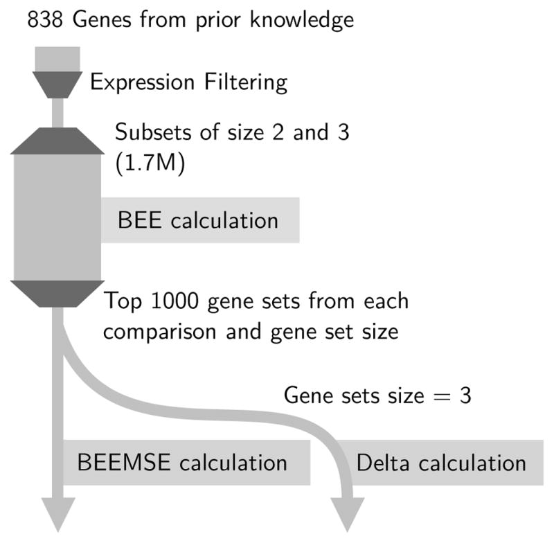
Classification of 858 genes from prior knowledge was performed with an expression filtration step, then BEE calculations were performed on all 1.7M gene sets across the three comparisons and two dimensionalities (sets of two and three genes). Then the lowest 1000 classification error sets were selected from each comparison and run in additional BEEMSE and calculations.

This filtering reduced the list of genes to be evaluated from the previously selected 858 to 185, 58, and 159 in the fpa-cpa, cpa-cca, and fpa-cca comparisons, respectively. Computing all two and three gene subsets of these three comparisons resulted in 1.7M BEE calculations to be performed over 200 cores over a period of several days.

Subsequently, the top 1000 gene sets from each comparison and dimensionality (two and three) were additionally used to perform BEEMSE and Δ computations.

The computations described in Section 2.3 consider the parameter c as a random variable. Consequently, we can also place a prior over c with all mass on a single value. This effectively treats c as a constant, known parameter. In this paper, because of the specific experimental design and the purpose of the OBC classification, i.e. to examine sets of genes that can discriminate well between the experimentally generated phenotypes, we assume c = 0.5. This choice reflects the experimental design that makes no a priori preference towards the classes being compared. Thus, we considered the error contribution from each class as equally important.

4 Results

4.1 Differential Expression Analysis

To establish a point of comparison Fig. 4 shows the distribution of un-adjusted P-values for the entire 12,000 genes in the fpa-cca comparison and of the 858 genes used in classification. The distribution of P-values for the 858 genes shows that most genes were not differentially expressed and the distribution of P-values was similar to that of the entire dataset.

Fig. 4.

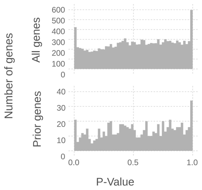
For the fpa-cca comparison the above histogram for all 12,000 genes and for the 858 genes in the prior knowledge gene list show that the majority of genes in the prior knowledge list set are not differentially expressed and have a distribution of P-values to the entire dataset.

Table 1 shows the top 10 genes from the 858 gene list as reported by adjusted P-value from DESeq. Using a traditional 0.05 threshold, only six genes would be considered statistically differentially expressed.

TABLE 1.

The top ten differentially expressed genes of the 858 gene list by adjusted P-value as reported by DESeq in the fpa-cca comparison.

Gene	Adjusted P-Value
Hoxa2	0.0001
Fabp1	0.0061
Nucks1	0.0085
Plaa	0.0227
P4hb	0.0227
Il6st	0.0250
Pax6	0.0517
Aldh2	0.0774
Ccndbp1	0.0784
Rxra	0.0867

4.2 Overall Error Distributions

The overall distributions of classification errors from a random sampling of the 300M possible gene sets from the 858 prior-knowledge-selected genes are given in Fig. 5 split across the number of genes used and the phenotype comparison.

Fig. 5.

The overall classification error distributions are shown by the number of features (panel x-axis), dietary comparison (panel y-axis), and normalization type (stacked plot colors). Average classification error is slightly lower (0.28 vs 0.30) as expected for classification with 3 genes when compared against two genes. Additionally, the three dietary comparisons (oil and fiber types (FP/CC), oil only (FP/CP), and fiber only (CP/CC)), showed differences in average classification performance.

Classification errors in the cpa-cca comparison are significantly higher than the other two groups. This matches previous qPCR data (not published) that also indicated greater transcriptional differences in animals fed dietary fat as opposed to fiber. It can also be noted that the three-gene sets show slightly lower classification errors on average than the two-gene sets.

Figure 6 shows the relationship between the BEE and the BEEMSE across this dataset. The figure shows that the BEE and BEEMSE are tightly correlated at low BEE values, and this correlation diminishes at higher values of the BEE.

Fig. 6.

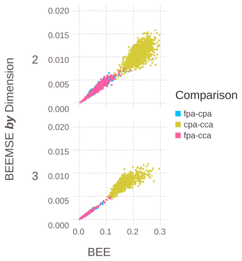
For the best 1000 gene sets for each dietary comparison, the BEEMSE tends to increase as a function of BEE.

More gene sets in the lower left of Fig. 6 indicates that the fpa-cca and fpa-cpa comparisons are well separated by a larger combination of genes than the cpa-cca comparison. The fewer number of gene sets in the lower left for the cpa-cca comparison indicates that the transcriptional differences between the phenotypes are small, we are considering the wrong set of genes, or the data for these phenotypes might contain a higher level of noise.

As more genes are used for classification, the points shift to the left and down as the dataset becomes more separable (if any such separation exists).

The top four gene pairs from each classification grouping are shown in Table 2. Genes such as Fabp1 are present both in this list for classification and in Table 1 as a differentially expressed gene for the fpa-cca comparison. Most other genes, however, have non-significant adjusted P-values, such as Arg2 (P=0.11, adjusted P=1.0) and Adamts1 (P=0.82, adjusted P=1.0), yet together can have classification errors of less than 1%. This is illustrated along with the OBC decision boundary in Fig. 7.

TABLE 2.

The top four lowest classification error gene sets for each of the three comparisons and for two and three genes. In addition, the Δ value for the three gene comparisons gives the reduction of classification error when adding the third gene to the best performing gene subset of size two. Errors, MSEs, and Δs below 0.01 are not displayed here due to the larger relative effects of Monte Carlo error at these value ranges.

Gene	Gene	Gene	P-Value	P-Value	P-Value	Comparison	ε̂	Var(ε|Sn)	Δ
Arg2	Adamts1		0.11	0.82		FPA-CCA	< 0.01	< 0.01
Adamts1	Lgals3bp		0.82	0.69		FPA-CCA	< 0.01	< 0.01
Fabp1	Arg2		0.00	0.11		FPA-CCA	< 0.01	< 0.01
Fgfr1	Adamts1		1.00	0.82		FPA-CCA	< 0.01	< 0.01
Arg2	Adamts1		0.11	0.82		FPA-CPA	< 0.01	< 0.01
Adamts1	Lgals3bp		0.82	0.69		FPA-CPA	< 0.01	< 0.01
Fabp1	Arg2		0.00	0.11		FPA-CPA	0.0125	< 0.01
Fabp1	Scd1		0.00	0.97		FPA-CPA	0.0127	< 0.01
Ccne1	Crabp2		0.99	0.93		CPA-CCA	0.1219	< 0.01
Ccne1	Bmp3		0.99	0.29		CPA-CCA	0.1311	< 0.01
Fabp1	Crabp2		0.00	0.93		CPA-CCA	0.1348	< 0.01
Ccne1	Tnfrsf12a		0.99	0.66		CPA-CCA	0.1366	< 0.01
Fabp1	Pde4b	P2rx2	0.00	0.45	0.95	FPA-CCA	< 0.01	< 0.01	< 0.01
Fabp1	Pde4b	Scd1	0.00	0.45	0.97	FPA-CCA	< 0.01	< 0.01	< 0.01
Fabp1	Pde4a	Pde4b	0.00	0.71	0.45	FPA-CCA	< 0.01	< 0.01	< 0.01
Fabp1	Pde4b	Arg2	0.00	0.45	0.11	FPA-CCA	< 0.01	< 0.01	< 0.01
Fabp1	Pde4b	P2rx2	0.00	0.45	0.95	FPA-CPA	< 0.01	< 0.01	< 0.01
Fabp1	Pde4a	Pde4b	0.00	0.71	0.45	FPA-CPA	< 0.01	< 0.01	< 0.01
Fabp1	Pde4b	Scd1	0.00	0.45	0.97	FPA-CPA	< 0.01	< 0.01	< 0.01
Fabp1	Pde4b	Fgfr1	0.00	0.45	1.00	FPA-CPA	< 0.01	< 0.01	< 0.01
Ccne1	Fabp1	Crabp2	0.99	0.00	0.93	CPA-CCA	0.0916	< 0.01	0.0312
Ccne1	Bmp3	Crabp2	0.99	0.29	0.93	CPA-CCA	0.0945	< 0.01	0.0348
Ccne1	Fabp6	Dpep1	0.99	0.38	0.98	CPA-CCA	0.0969	< 0.01	0.0399
Ccne1	Dpep1	Abcb1a	0.99	0.98	0.34	CPA-CCA	0.0969	< 0.01	0.0449

Fig. 7.

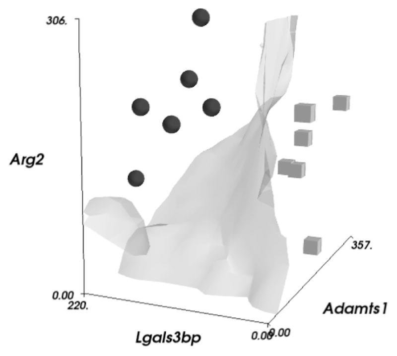
Normalized count expressions are shown for the three genes Arg2, Lgals3bp, and Adamts1. The cubes and spheres indicate the fpa and cca samples, respectively. Using the marching cubes contouring algorithm, an approximate rendering of the nonlinear OBC decision boundary is also displayed.

For classifications using gene sets of size three, we compute Δ to show the amount of classification improvement by adding an additional gene. Figure 8 shows the distribution of Δ for the three comparison groups. Because the cpa-cca comparison has the highest classification errors it shows the largest improvements (> 0.02) by adding an additional feature to the classification problem.

Fig. 8.

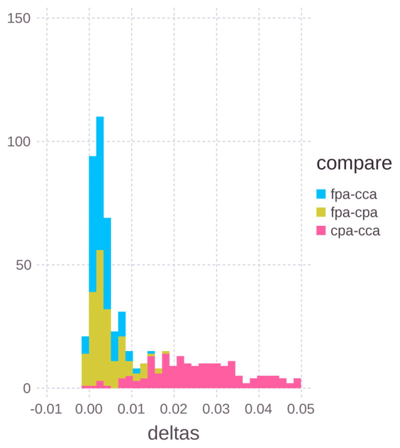
The distribution of Δ for the top 1000 gene sets of the three comparison groups. CPA-CCA has the largest Δ values which corresponds to that comparison having the largest classification errors. Negative values of Δ are due to approximation error.

One concern with using approximation algorithms is whether the computation is sufficiently repeatable. To address this, we ran the top 200 gene subsets from each comparison twice and computed the correlation of BEE estimates from the two runs. A Pearson correlation coefficient of 0.999 across the six comparisons indicated that the computation is repeatable.

Figure 9 shows the comparison between no normalization, count-based normalization, and model-based normalization. The normalized counts show an increase in classification error, potentially due to the 2% rounding error induced from the final integer conversion.

Fig. 9.

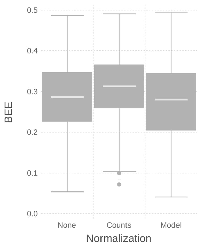
Overall classification error varied depending on whether normalization was used (None) and whether it was implemented as a pre-processing step applied to the data (Counts) or input into the model through the sequencing depth variable d (Model).

4.3 Biological Findings

The interactions of dietary fiber-derived compounds in the colonic lumen can have a substantial impact on the metabolism and kinetics of the colon epithelial cell population and suppress inflammation and neoplasia [20], [21]. It has been proposed by us and others that n-3 PUFA found in fish oil and butyrate (a fiber fermentation product) interact in the colon to profoundly suppress colon cancer [22], [23].

We found that in the chemoprotective treatment containing fish oil and fermentable fiber (FPA-CCA), two genes, Fabp1 and Eno3, were prominently detected together with a wide variety of other genes in the gene sets of length three. The calculated 23 fold over-expression of Fabp1 correlates with previous findings classifying Fabp1 as a tumor suppressor in colon cancer [24], [25]. Since Fabp1 is a gene involved in the uptake and metabolic processing of PUFA, the higher levels of fish oil derived n-3 PUFA are the most likely cause for its increased expression and chemoprotective activity [26]. The 1.3 fold upregulation of Eno3 is likely due to the fermentable fiber in the diet. Fermentable fiber leads to the generation of the HDAC inhibitor butyrate, which has been previously associated with concurrent increases in enolase 3 (Eno3) levels and differentiation, a hallmark of chemoprotection [27], [28]. The expression levels of Fabp1 and Eno3 are shown along with the OBC classification boundary in Fig. 10.

Fig. 10.

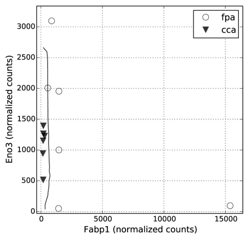
Normalized counts of the Fabp1 and Enoff genes were plotted against each other in relation to the OBC decision boundary (black line) for the fpa-cca comparison.

Other genes present with Fabp1 and Eno3 included Ccnd2 (BEE=0.018), Arg2 (BEE=0.004) and Cdk1 (BEE=0.014). Ccnd2, a gene responsible for enhancing cancer cell proliferation, was downregulated by 1.4 fold in the FPA chemoprotective diet. Similarly, anti-oncogenic genes Arg2 and Cdk1 were also present in low-classification gene sets of size three and these were elevated by 3.34 fold and 1.28 fold, respectively, in the FPA diet. Both of these genes can be upregulated by HDAC inhibitors, a putative mechanism for the chemoprotective nature of these diets [29], [30].

Although these three genes were not considered differentially expressed through individual testing (P-values of 0.11, 0.36, and 0.51 for Arg2, Ccnd2, and Cdk1, respectively), they were indicated as highly predictive in delineating the phenotype when using the Bayesian error estimator. These data suggest that via multivariate interactions with other genes, the BEE highlights novel genes for the purposes of hypothesis generation or further biomarker development/validation. This supports the biological relevance of the BEE as a useful tool in RNA-seq analysis.

5 Conclusion

This work demonstrates an application of the OBC and BEE in identifying multivariate gene interactions in RNA-Seq data for the purpose of differentiating biological phenotypes.

Using 858 genes selected by prior knowledge in a pre-clinical RNA-Seq dataset, we identified genes that in combination yield low classification errors, whereas each gene individually had a large P-value for differential expression. Thus, the application of our previously developed Bayesian classification framework [4] enables investigators to generate new hypotheses regarding multivariate effects between these gene sets and the observed phenotypes.

In addition, new tools such as BEE-BEEMSE scatter plots offer additional diagnostic visualizations to assess the quality of RNA-Seq data, similarly to a volcano plots, as done in DE testing. Future work needs to be performed on synthetic data sets to better uncover the utility of such a graphical representation of the classification performance. Computing and reporting the classification improvements as represented by the Δ quantity is also of particular interest to biologists as large values could potentially indicate more complex interactions between genes than merely P-values or even BEE alone can.

Biographies

Jason Knight Jason Knight is a Ph.D. student in the Electrical and Computer Engineering Department at Texas A&M University. His research interests are in using Bayesian statistical models and high performance computing to develop new methods to analyze high throughput biological data. Specifically, through the use of model-based statistics, domain knowledge in the form of prior distributions can be applied to the high dimensional, nonlinear phenomena that pervade biology.

Karen Triff Karen Triff is a Ph.D. student in the Biology Department at Texas A&M University where she studies the chemoprotective effects of dietary fatty acids and fibers. She utilizes ChIP-Seq and RNA-Seq techniques on animal models for carcinogenesis in the colon. Through genome-wide approaches she studies the epigenetic and transcriptional regulation of these diets and their chemo-protective effects.

Ivan Ivanov Dr. Ivan Ivanov received his Ph.D. (Mathematics) from the University of South Florida in 1999. He was a Research Professor at the Mathematics Department of Syracuse University (1999 – 2000), at the Mathematics Department, Texas A&M University (2000 –2003), and a postdoctoral trainee in the Training Program in Bioinformatics at Texas A&M University (2003 – 2005). He is currently a Clinical Associate Professor in the Department of Veterinary Physiology and Pharmacology at Texas A&M University and serves as the Director of the Quantitative Biology Core in the Center for Translational and Environmental Health Research. His research interest focus is in several key areas of computational biology and toxicology: (i) System identification and inference from genome-wide data, (ii) Model complexity reduction and compression, (iii) Control of the dynamical behavior for the purposes of therapeutic intervention, and (iv) Design of predictive computational models for cell response to nanomaterial exposure.

Robert Chapkin Dr. Chapkin is an expert in environmental modulators related to chemoprevention of colon cancer and chronic inflammatory diseases, e.g., inflammatory bowel disease. He has been continuously funded by NIH/NCI for the past 25 years and has made highly significant contributions to T cell/inflammation biology and cancer chemoprevention in five specific areas: (i) membrane biology and nutritional modulation of epithelia/immune cell membrane structure and function, (ii) establishment of models for chronic inflammation and cancer prevention studies, (iii) elucidation of signal transduction processes in intestinal stem cells, (iv) investigation of the role of inflammation as a critical factor in cancer development, and its modulation by diet, and (v) development of novel noninvasive Systems Biology-based methodologies to assess crosstalk between the gut microbiome and the host transcriptome and its application to translational research. He serves as the Deputy Director of the P30 NIEHS sponsored Texas A&M Center for Translational Environmental Health Research (CTEHR) and coordinates the Quantitative Biology Core.

Ed Dougherty Edward R. Dougherty is a Distinguished Professor in the Department of Electrical and Computer Engineering at Texas A&M University in College Station, TX, where he holds the Robert M. Kennedy ‘26 Chair in Electrical Engineering and is Scientific Director of the Center for Bioinformatics and Genomic Systems Engineering. He holds a Ph.D. in mathematics from Rutgers University and an M.S. in Computer Science from Stevens Institute of Technology, and has been awarded the Doctor Honoris Causa by the Tampere University of Technology. He is a fellow of both IEEE and SPIE, has received the SPIE President’s Award, and served as the editor of the SPIE/IS&T Journal of Electronic Imaging. At Texas A&M University he has received the Association of Former Students Distinguished Achievement Award in Research, been named Fellow of the Texas Engineering Experiment Station and Halliburton Professor of the Dwight Look College of Engineering. Prof. Dougherty is author of 16 books and author of more than 300 journal papers.

References

- 1.Trapnell C, Roberts A, Goff L, Pertea G, Kim D, Kelley DR, Pimentel H, Salzberg SL, Rinn JL, Pachter L. Differential gene and transcript expression analysis of RNA-seq experiments with TopHat and Cufflinks. Nature protocols. 2012;7(3):562–578. doi: 10.1038/nprot.2012.016. [DOI] [PMC free article] [PubMed] [Google Scholar]
- 2.Robinson MD, McCarthy DJ, Smyth GK. edgeR: A Bioconductor package for differential expression analysis of digital gene expression data. Bioinformatics. 2010;26(1):139–140. doi: 10.1093/bioinformatics/btp616. [DOI] [PMC free article] [PubMed] [Google Scholar]
- 3.Love MI, Huber W, Anders S. Moderated estimation of fold change and dispersion for RNA-Seq data with DESeq2. 2014 doi: 10.1186/s13059-014-0550-8. bioRxiv. [DOI] [PMC free article] [PubMed] [Google Scholar]
- 4.Knight JM, Ivanov I, Dougherty ER. MCMC implementation of the optimal Bayesian classifier for non-Gaussian models: model-based RNA-Seq classification. BMC bioinformatics. 2014;15(1):401. doi: 10.1186/s12859-014-0401-3. [DOI] [PMC free article] [PubMed] [Google Scholar]
- 5.Dalton LA, Dougherty ER. Optimal classifiers with minimum expected error within a Bayesian framework – Part I: Discrete and Gaussian models. Pattern Recognition. 2013;46(5):1301– 1314. [Online]. Available: http://www.sciencedirect.com/science/article/pii/S0031320312004529. [Google Scholar]
- 6.Dalton LA, Dougherty ER. Optimal classifiers with minimum expected error within a Bayesian framework – Part II: Properties and performance analysis. Pattern Recognition. 2013;46(5):1288–1300. Online Available: http://www.sciencedirect.com/science/article/pii/S0031320312004530. [Google Scholar]
- 7.Dalton LA, Dougherty ER. Bayesian minimum mean-square error estimation for classification error – Part I: Definition and the Bayesian MMSE error estimator for discrete classification. Signal Processing, IEEE Transactions on. 2011;59(1):115–129. [Google Scholar]
- 8.Dalton LA, Dougherty ER. Bayesian minimum mean-square error estimation for classification error – Part II: the Bayesian MMSE error estimator for linear classification of Gaussian distributions. IEEE Transactions on Signal Processing. 2011;59:130–144. [Google Scholar]
- 9.Dalton LA, Dougherty ER. Exact sample conditioned MSE performance of the Bayesian MMSE estimator for classification error—Part I: Representation. Signal Processing, IEEE Transactions on. 2012;60(5):2575–2587. [Google Scholar]
- 10.Katz Y, Wang ET, Airoldi EM, Burge CB. Analysis and design of RNA sequencing experiments for identifying isoform regulation. Nature methods. 2010;7(12):1009–1015. doi: 10.1038/nmeth.1528. [DOI] [PMC free article] [PubMed] [Google Scholar]
- 11.Ghaffari N, Yousefi MR, Johnson CD, Ivanov I, Dougherty ER. Modeling the next generation sequencing sample processing pipeline for the purposes of classification. BMC bioinformatics. 2013;14(1):307. doi: 10.1186/1471-2105-14-307. [DOI] [PMC free article] [PubMed] [Google Scholar]
- 12.Owen AB. Monte Carlo theory, methods and examples. 2013 [Google Scholar]
- 13.Dillies MA, Rau A, Aubert J, Hennequet-Antier C, Jeanmougin M, Servant N, Keime C, Marot G, Castel D, Estelle J, et al. A comprehensive evaluation of normalization methods for Illumina high-throughput RNA sequencing data analysis. Briefings in bioinformatics. 2013;14(6):671–683. doi: 10.1093/bib/bbs046. [DOI] [PubMed] [Google Scholar]
- 14.Liang F, Liu C, Carroll R. Advanced Markov chain Monte Carlo methods: learning from past samples. Vol. 714 Wiley; 2011. [Google Scholar]
- 15.Brooks SP, Gelman A. General methods for monitoring convergence of iterative simulations. Journal of computational and graphical statistics. 1998;7(4):434–455. [Google Scholar]
- 16.Cowles MK, Carlin BP. Markov chain Monte Carlo convergence diagnostics: a comparative review. Journal of the American Statistical Association. 1996;91(434):883–904. [Google Scholar]
- 17.Dobin A, Davis CA, Schlesinger F, Drenkow J, Zaleski C, Jha S, Batut P, Chaisson M, Gingeras TR. STAR: Ultrafast Universal RNA-seq aligner. Bioinformatics. 2013;29(1):15–21. doi: 10.1093/bioinformatics/bts635. [DOI] [PMC free article] [PubMed] [Google Scholar]
- 18.Anders S, Pyl PT, Huber W. HTSeq–A Python framework to work with high-throughput sequencing data. 2014 doi: 10.1093/bioinformatics/btu638. bioRxiv. [DOI] [PMC free article] [PubMed] [Google Scholar]
- 19.Zhao C, Ivanov I, Dougherty ER, Hartman TJ, Lanza E, Bobe G, Colburn NH, Lupton JR, Davidson LA, Chapkin RS. Noninvasive detection of candidate molecular biomarkers in subjects with a history of insulin resistance and colorectal adenomas. Cancer Prevention Research. 2009;2(6):590–597. doi: 10.1158/1940-6207.CAPR-08-0233. [DOI] [PMC free article] [PubMed] [Google Scholar]
- 20.Cho Y, Kim H, Turner ND, Mann JC, Wei J, Taddeo SS, Davidson LA, Wang N, Vannucci M, Carroll RJ, et al. A chemoprotective fish oil-and pectin-containing diet temporally alters gene expression profiles in exfoliated rat colonocytes throughout oncogenesis. The Journal of nutrition. 2011;141(6):1029–1035. doi: 10.3945/jn.110.134973. [DOI] [PMC free article] [PubMed] [Google Scholar]
- 21.Kolar S, Barhoumi R, Jones CK, Wesley J, Lupton JR, Fan YY, Chapkin RS. Interactive effects of fatty acid and butyrate-induced mitochondrial Ca2+ loading and apoptosis in colonocytes. Cancer. 2011;117(23):5294–5303. doi: 10.1002/cncr.26205. [DOI] [PMC free article] [PubMed] [Google Scholar]
- 22.Davidson LA, Nguyen DV, Hokanson RM, Callaway ES, Isett RB, Turner ND, Dougherty ER, Wang N, Lupton JR, Carroll RJ, et al. Chemopreventive n-3 polyunsaturated fatty acids reprogram genetic signatures during colon cancer initiation and progression in the rat. Cancer Research. 2004;64(18):6797–6804. doi: 10.1158/0008-5472.CAN-04-1068. [DOI] [PMC free article] [PubMed] [Google Scholar]
- 23.Chapkin RS, Seo J, McMurray DN, Lupton JR. Mechanisms by which docosahexaenoic acid and related fatty acids reduce colon cancer risk and inflammatory disorders of the intestine. Chemistry and physics of lipids. 2008;153(1):14–23. doi: 10.1016/j.chemphyslip.2008.02.011. [DOI] [PMC free article] [PubMed] [Google Scholar]
- 24.Lawrie L, Dundas S, Curran S, Murray G. Liver fatty acid binding protein expression in colorectal neoplasia. British journal of cancer. 2004;90(10):1955–1960. doi: 10.1038/sj.bjc.6601828. [DOI] [PMC free article] [PubMed] [Google Scholar]
- 25.Satoh Y, Mori K, Kitano K, Kitayama J, Yokota H, Sasaki H, Uozaki H, Fukayama M, Seto Y, Nagawa H, et al. Analysis for the combination expression of CK20, FABP1 and MUC2 is sensitive for the prediction of peritoneal recurrence in gastric cancer. Japanese journal of clinical oncology. 2011:hyr179. doi: 10.1093/jjco/hyr179. [DOI] [PubMed] [Google Scholar]
- 26.Norris AW, Spector AA. Very long chain n-3 and n-6 polyunsaturated fatty acids bind strongly to liver fatty acid-binding protein. Journal of lipid research. 2002;43(4):646–653. [PubMed] [Google Scholar]
- 27.Stierum R, Gaspari M, Dommels Y, Ouatas T, Pluk H, Jespersen S, Vogels J, Verhoeckx K, Groten J, Ommen Bv. Proteome analysis reveals novel proteins associated with proliferation and differentiation of the colorectal cancer cell line Caco-2. Biochimica et Biophysica Acta (BBA)-Proteins and Proteomics. 2003;1650(1):73–91. doi: 10.1016/s1570-9639(03)00204-8. [DOI] [PubMed] [Google Scholar]
- 28.Valentini A, Biancolella M, Amati F, Gravina P, Miano R, Chillemi G, Farcomeni A, Bueno S, Vespasiani G, Desideri A, et al. Valproic acid induces neuroendocrine differentiation and UGT2B7 up-regulation in human prostate carcinoma cell line. Drug metabolism and disposition. 2007;35(6):968–972. doi: 10.1124/dmd.107.014662. [DOI] [PubMed] [Google Scholar]
- 29.Leone V, D’Angelo D, Rubio I, de Freitas PM, Federico A, Colamaio M, Pallante P, Medeiros-Neto G, Fusco A. MiR-1 is a tumor suppressor in thyroid carcinogenesis targeting CCND2, CXCR4, and SDF-1α. The Journal of Clinical Endocrinology & Metabolism. 2011;96(9):E1388–E1398. doi: 10.1210/jc.2011-0345. [DOI] [PubMed] [Google Scholar]
- 30.Pandey D, Sikka G, Bergman Y, Kim JH, Ryoo S, Romer L, Berkowitz D. Transcriptional Regulation of Endothelial Arginase 2 by Histone Deacetylase 2. Arteriosclerosis, thrombosis, and vascular biology. 2014:ATVBAHA–114. doi: 10.1161/ATVBAHA.114.303685. [DOI] [PMC free article] [PubMed] [Google Scholar]
- 31.Bezanson J, Karpinski S, Shah VB, Edelman A. Julia: A fast dynamic language for technical computing. 2012 arXiv preprint arXiv:1209.5145. [Google Scholar]
- 32.Bezanson J, Karpinski S, Shah VB, Fischer K, Nash J, Nolta M, Holy T, Baldassi C, Saba E, Chen J, Johnson SG, Noack A, Boyer S, Squire K, O’Leary P, Lin D, Bates D, Kornblith S, Isaiah, Murthy A, Kelman T, Quinn J, Andrioni A, Xing G, Mohapatra T, Byrne S, Sengupta A, Bauman M, White JM, Nesje I. julia v0.3.0. 2014 Aug; [Online]. Available: http://dx.doi.org/10.5281/zenodo.11355.
- 33.Jones D, Chudzicki D, Sengupta A, Darakananda D, Holy T, Kleinschmidt D, Fischer K, Dunning I, verzani john, Coalson C, Karpinski S, Zwitch R, Forsyth J, Saba E, Garborg S, Johnson B, Mesecke S, Eglen S, Mackesey Adrián S, Ennis RJ, Schauer M, Chen J, Merrill J, Knight J, Nesje I, Lin D inkyu, nignatiadis, powerdistribution. Gadfly.jl: Version 0.3.9. 2014 Sep; [Online]. Available: http://dx.doi.org/10.5281/zenodo.11876.