A fuzzy based feature selection from independent component subspace for machine learning classification of microarray data

Abstract

Feature (gene) selection and classification of microarray data are the two most interesting machine learning challenges. In the present work two existing feature selection/extraction algorithms, namely independent component analysis (ICA) and fuzzy backward feature elimination (FBFE) are used which is a new combination of selection/extraction. The main objective of this paper is to select the independent components of the DNA microarray data using FBFE to improve the performance of support vector machine (SVM) and Naïve Bayes (NB) classifier, while making the computational expenses affordable. To show the validity of the proposed method, it is applied to reduce the number of genes for five DNA microarray datasets namely; colon cancer, acute leukemia, prostate cancer, lung cancer II, and high-grade glioma. Now these datasets are then classified using SVM and NB classifiers. Experimental results on these five microarray datasets demonstrate that gene selected by proposed approach, effectively improve the performance of SVM and NB classifiers in terms of classification accuracy. We compare our proposed method with principal component analysis (PCA) as a standard extraction algorithm and find that the proposed method can obtain better classification accuracy, using SVM and NB classifiers with a smaller number of selected genes than the PCA. The curve between the average error rate and number of genes with each dataset represents the selection of required number of genes for the highest accuracy with our proposed method for both the classifiers. ROC shows best subset of genes for both the classifier of different datasets with propose method.

1. Introduction

Gene expression analysis using microarrays has become an important part of biomedical and clinical research. Recent advancements in DNA microarray technology have enabled us to monitor and evaluate the expression levels of thousands of genes simultaneously, which allows a great deal of microarray data to be generated [1]. Microarray techniques have been successfully employed virtually in every aspect of biomedical research because they exhibit the possibility to do massive tests on genome patterns [2]. Microarray gene expression data usually has a large number of dimensions and is permitted to evaluate each gene in a single environment in different types of tissues like various cancerous tissues [3]. Accordingly, microarray data analysis, which can supply useful data for cancer prediction and diagnosis, has also attracted many researchers from diverse areas. Progressively, the challenge is to translate such data to get a clear insight into biological processes and the mechanisms of human disease [4]. To aid such discoveries, mathematical and computational tools are required that are versatile enough to capture the underlying biology and simple enough to be applied efficiently on large datasets. Therefore, novel statistical methods must be introduced to analyze those large amounts of data generated from microarray experiments [5]. The process of microarray classification consists of two successive steps. The first step is to select a set of significant and relevant genes and the second step is to develop a classification model, which can produce accurate prediction for unseen data. One of the key goals of microarray data analysis is to distinguish the various categories of cancers. A true and accurate classification is essential for successful diagnosis and treatment of cancer. The enormous dimensionality of the DNA microarray data becomes a problem, when it is employed for cancer classification, as the sample size of DNA-microarray is far less than the gene size [6]. However, among the large number of genes, only a small fraction is effective for performing a classification task, so the choice of relevant genes is an important task in most microarray data studies that will give higher accuracy for sample classification (for example, to distinguish cancerous from normal tissues). This trouble can be alleviated by using machine learning with a gene selection problem. The goal of gene selection methods is to determine a small subset of informative genes that reduces processing time and provides higher classification accuracy [7]. There are a large number of methods, which have been developed and applied to do gene selection. A typical gene selection method has two constituents, an evaluation criterion and a searching scheme. As many evaluation criteria and searching schemes already exist, it is possible to develop many gene selection methods by just combining different evaluation criteria and searching schemes. Since, many of these combinations of evaluation criteria and searching schemes actually perform similarly, it is sufficient to compare the most commonly used combinations instead of all possible combinations [8]. The commonly used gene selection & extraction approaches are t-test, Relief-F, information gain, SNR-test and principal component analysis (PCA), linear discriminant analysis, independent component analysis (ICA). These methods are capable of selecting a smaller subset of genes for sample classification [9]. Recently, independent component analysis (ICA) method has received growing attention as effective data-mining tools for microarray gene expression data. As a technique of higher-order statistical analysis, ICA is capable of extracting biologically relevant gene expression features of microarray data [10]. The success of the ICA method depends upon the appropriate choice of best gene subset from given ICA feature vector and choice of an appropriate classifier [11].

In this study, fuzzy backward feature elimination (FBFE) scheme was introduced, in which features were eliminated successively from ICA feature vector according to their influence on a SVM and NB based evaluation criterion. FBFE is a backward feature elimination method based on fuzzy entropy measure. Several machine learning techniques, such as artificial neural networks (ANN), k-nearest neighbor (KNN), support vector machine (SVM), Naïve Bayes (NB), decision tree, random forest and kernel-based classifiers, have been successfully applied to microarray data and also for other biological data analyses in recent years [4], [12]. From the study of Liwei Fan et al. and Chun-Hou Zheng, it was seen that NB and SVM were the best classifiers with ICA for microarray data, and feature subset selection from the ICA feature vector can significantly improve the performance of classifiers [3], [13].

Naïve Bayes (NB) classifier is a simple Bayesian network classifier, which is built upon the firm assumption that different attributes are independent of each other in the given course of instruction. There are two major challenges that may seriously affect the successful application of NB classifier to microarray data analysis. The first is the conditional independence assumption rooted in the classifier itself, which is hardly satisfied by the microarray data [14]. This limitation could be successfully resolved as the components extracted by the ICA are statistically independent therefore, gene extraction by ICA could effectively improve the performance of a NB classifier for microarray data. Second limitation is that, all the attributes have an influence on the classification; hence, the use of FBFE eliminates the inappropriate genes from ICA feature vector to improve the performance of a NB classifier during cross validation. It is therefore necessary to select genes to reduce the dimensionality of microarray data before applying a NB classifier [15]. On the other hand the SVM-based classifier is superior, as it is less sensitive to the curse of dimensionality and more robust than other non-SVM classifiers [16]. The biggest drawback of an SVM is that it cannot directly obtain the genes of importance. Thus, during the fitting of an SVM model, a careful gene selection has to be done first and then the selected genes should be used to obtain improved classification results. If genes are not appropriately chosen, there may be a large number of redundant variables in the model, severely affecting its performance [17].

In this paper, a fuzzy backward feature elimination (FBFE) approach is used to eliminate the inappropriate genes from the independent components of the DNA microarray data for support vector machine (SVM) and Naïve Bayes (NB) classifiers. The proposed approach consists mainly of two steps. The original DNA microarray gene expression data are modeled by independent component analysis (ICA), and then the most discriminant features extracted by the ICA are selected by the fuzzy feature selection technique, which will be introduced and discussed in detail in Section 2. The next section explains the classification procedure of SVM and NB, followed by the details of used datasets and preprocessing step of datasets. In Section 4, the proposed method is compared and evaluated with PCA as a standard extraction method on several microarray datasets. The experimental results on five microarray datasets, show that the proposed approach can, not only improve the average classification accuracy rates, but also reduce the variance in classification performance of SVM and NB. Discussions and conclusions are presented in Section 5.

2. Proposed approach

2.1. Feature extraction by ICA

ICA is a projection method that linearly decomposes the dataset into components that have a desired property. ICA decomposes an input dataset into components such that each component is statistically as independent from the others as possible, which was proposed by Hyvarinen and has been proven successful in many applications [18]. ICA is an extension of PCA; PCA projects the data into a new space spanned by the principal components. In contrast to PCA, the goal of ICA is to find a linear representation of non-Gaussian data so that the components are statistically independent [19]. ICA provides a more biologically plausible model for gene expression data by assuming a non-Gaussian data distribution. ICA provides a data-driven method for exploring functional relationships and grouping genes into transcriptional modules.

In the simplest form of ICA, the expression levels of all genes are taken as n scalar random variables x₁, x₂, …, x_n, which are assumed to be linear combinations of m unknown independent components S₁, S₂, …, S_m that is mutually statistically independent, and possess zero-mean. Let the expression levels x_j be arranged into a vector X = (x₁, x₂, …, x_n)^T which are modeled as linear combination of m random variable S = (s₁, s₂, …, s_m)^T [20]:

$$x_j=a_{j1}{s}_1+a_{j2}{s}_2+\dots +a_{\mathit{jm}}{s}_m,\mathrm{for}\mathrm{all}j=1,\dots ,n$$ (1)

$$X=\mathit{AS},\left[\begin{array}{l}{x}_1\\ .\\ .\\ \\ x_n\end{array}\right]=\left[\begin{array}{cccc}\hfill a_{11}\hfill & \hfill .\hfill & \hfill .\hfill & \hfill a_{1m}\hfill \\ \hfill \begin{array}{l}.\\ .\end{array}\hfill & \hfill \hfill & \hfill \hfill & \hfill .\hfill \\ \hfill .\hfill & \hfill \hfill & \hfill \hfill & \hfill .\hfill \\ \hfill a_{n1}\hfill & \hfill \hfill & \hfill \hfill & \hfill a_{\mathit{nm}}\hfill \end{array}\right]\left[\begin{array}{l}{s}_1\\ .\\ .\\ .\\ s_m\end{array}\right]$$ (2)

where X, is (n × m) matrix which denotes microarray gene expression data, with n genes and m samples, and a_ij (i = 1, … , m) in X are some real ratio of intensities, represent the expression level of ith genes in the jth sample, and number of genes are much greater than that of the sample m i.e., n ≫ m. This is a basic ICA model of microarray gene expression data. It is assumed that the observed variables are independent components, these are latent variable, which cannot be directly observed and the mixing matrix A is also assumed to be unknown matrix. The random variable x_j is known and both matrices S and A using X are to be estimated. In most cases, to simplify feature selection, the number of features is always assumed to be equal to the number of observed variables, n = m. Then, the mixing matrix A becomes an m × m square matrix and can invert the mixing matrix as:

$$U=S=A^{-1}X=\mathit{WX}.$$ (3)

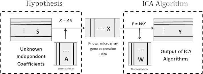
Then ICA can be applied to find a matrix W that provides the transformation U = u₁ , u₂ , … , u_m = WX of the observed matrix X under which, the transformed random variables u₁ , u₂ , … , u_m called the independent components are as independent as possible. Theoretical framework of ICA algorithms of microarray gene expression data is shown in Fig. 1, as previously demonstrated by Wei Kong et al. [21].

Fig. 1.

Theoretical framework of ICA algorithms of microarray gene expression data.

A fixed point algorithm is a computationally highly efficient method for performing the estimation of ICA for microarray data [22]. It is based on a fixed-point iteration scheme that has been found in independent experiments to be 10–100 times faster than conventional gradient descent methods for ICA. In the fixed point algorithm of ICA (FastICA), maximizing negentropy is used as the contrast function since negentropy is an excellent measure of non-Gaussianity and is approximated by

$$J\left(u\right)=H\left(u_G\right)-H\left(u\right)$$ (4)

where u_G is a Gaussian random vector of the same covariance matrix as vector u, H is marginal entropy, which is defined as $H\left(u_i\right)=-{\displaystyle \int p\left(s_i\right)}logp\left(s_i\right)\text{d}{s}_i$ of the variable u_i and p(.) is a probabilistic density function. Mutual information I, is known as natural measure independence of random variables, it is widely used as the criterion in ICA algorithm and can be measured by

$$I=J\left(u\right)-{\displaystyle {\sum }_{i}J\left(u_i\right)}.$$ (5)

The independent components are determined, when mutual information I is minimized. From Eq. (5), it is clearly shown that minimizing the mutual information I is equivalent to maximizing the negentropy J(u). To estimate the negentropy of u_i = w^Tx, an approximation to identify independent components one by one is designed as follows:

$$J_G\left(w\right)={\left[E\left\{G\left(w^{T}x\right)\right\}-E\left\{G\left(v\right)\right\}\right]}^2$$ (6)

where, G can be practically any non-quadratic function, E(.) denotes the expectation, and v is a Gaussian variable of zero mean and unit variance [23].

2.2. Feature selection by FBFE technique

Fuzzy feature selection approach is used to select the best gene subset from the ICA feature vector for good separability of the classification task. A central issue associated with ICA is that it generally extracts a number of components, which are equal to the observational variables m for which again 2^m gene subsets exist [11]. The evaluation of all possible gene subsets leads to computational problem for large values of m. To solve this problem of identifying the most relevant feature subsets FBFE technique is applied.

Fuzzy feature selection is based on a fuzzy entropy measure. Since the fuzzy entropy is able to discriminate pattern distribution better, it is employed to evaluate the separability of each feature. Intuitively, the lower the fuzzy entropy of a feature, the higher is the feature's discriminating ability. Pasi Luukka suggested that corresponding to Shannon probabilistic entropy, the measure of fuzzy entropy should be [24]:

$$H_1\left(A\right)=-{\displaystyle \sum _{j=1}^n\left({\mu }_A\left(x_j\right)log{\mu }_A\left(x_j\right)+\left(1-{\mu }_A\left(x_j\right)\right)log\left(1-{\mu }_A\left(x_j\right)\right)\right)}$$ (7)

where μ_A(x_j) are the fuzzy values. This fuzzy entropy measure is considered to be a measure of fuzziness, and it evaluates global deviations from the type of ordinary sets, i.e. any crisp set A₀ lead to h (A₀) = 0. Note that the fuzzy set A with μ_A(x_j) = 0.5 plays the role of the maximum element of the ordering defined by H. Newer fuzzy entropy measures were introduced by Parkash et al. [25] where fuzzy entropies were defined as:

$$H_2\left(A:w\right)={\displaystyle \sum _{j=1}^n{w}_j\left(sin\frac{\pi {\mu }_A\left(x_j\right)}{2}+sin\frac{\pi \left(1-\pi {\mu }_A\left(x_j\right)\right)}{2}-1\right)}$$ (8)

$$H_3\left(A:w\right)={\displaystyle \sum _{j=1}^n{w}_j\left(cos\frac{\pi {\mu }_A\left(x_j\right)}{2}+cos\frac{\pi \left(1-\pi {\mu }_A\left(x_j\right)\right)}{2}-1\right)}.$$ (9)

These fuzzy entropy measures were used in the feature selection process. The main idea is, first to create the ideal vectors V_i = (v_i(f₁), …, v_i(f_t)) that represents the class i as well as possible. This vector can be user defined or calculated from some sample set X_i of vectors x = (x(f₁), …, x(f_t)) which are known to belong to class C_i. Here the generalized mean is used to create these class ideal vectors. Then the similarities S (x, V_i), between the sample x and the ideal vectors V_i are calculated. In calculating the similarity of the sample vectors and ideal vectors, j similarities are obtained, where j is the number of features. Then those similarities are collected into one similarity matrix. At this step, using the Eq. (7) entropy is calculated to evaluate the relevance of the features. Low entropy values are obtained if similarity values are high and if similarity values are close to 0.5, high entropy values are obtained. Using this underlying idea, the fuzzy entropy values can be calculated for features by using similarity values between the ideal vectors and sample vectors which are to be classified [26]. After the fuzzy entropy of each feature has been determined, the features can be selected by forward selection or backward elimination. The forward selection method is to select the relevant features beginning with an empty set and iteratively add features until the termination criterion is met. In contrast, the backward elimination method starts with the full feature set and removes features until the termination criterion is met [27]. In this paper a backward elimination method is used to pick the relevant features.

2.3. Performance evaluation method (LOOCV)

The Leave-One-Out Cross-Validation (LOOCV), performance is applied to characterize the behaviour of both the base classifiers. Two typical cross-validation methods (namely k-fold cross-validation and leave-one-out validation) have been widely used in microarray data classification evaluation. Comparing to the k-fold cross-validation method, the LOOCV method is more applicable due to the small sample size of microarray data [4], [9], [11], [28]. In LOOCV method of cross validation the number of partitions of a dataset is equal to the number of sample size (m). Each test set consists of a different singleton set and each training set consists of all (m − 1) cases not in the corresponding test set. Given a dataset containing m samples (m − 1) samples are used to construct a classifier and then apply the remaining one data sample to test this classifier. By repeating this process of successively using each data sample (x_i) as the testing data sample, totally m prediction e_i = c(x_i) (i = 1 − m) is obtained. The performance of the classifier is then measured by the average misclassification rate:

$$\mathit{Er}=\frac{1}{m}{\displaystyle \sum _{i=1}^m\delta \left(e_i,y_i\right)},$$

where y_i is the true class label, for instance x_i, and

$$\delta \left(x,y\right)=\begin{array}{ll}0\hfill & \text{if}x=y\hfill \\ 1\hfill & \text{if}x\ne y\hfill \end{array}.$$

2.4. SVM classifier

The support vector machine (SVM) is a popular algorithm for solving, pattern recognition, regression and density estimation problems, and perform better than most of the machine learning algorithms introduced by Vapnik and co-workers [29], [30], [31]. The SVM is a linear classifier that maximizes the margin between the separating hyperplane and the training data points. In case of linearly separable data, the goal of training phase of SVM is to find the linear function [32]:

$$f\left(x\right)=W^{T}X+b.$$ (10)

For the given training dataset that consists of n samples, (x_i, y_i) for i = 1, 2, …, n, x_i ∈ R^d represents input vectors and y_i denotes the class label of the ith sample. In the binary SVM the class label y_i is either 1 or − 1 i.e. y_i ∈ (− 1, + 1), Eq. (10) is the border for two different data classes and divides the space into two classes according to the condition:

W^TX + b > 0, W^TX + b < 0, where W ∈ Rⁿ is a normal vector, the bias b is a scalar; the separating plane is defined by W^TX + b = 0, and the distance between the two parallel hyperplanes is equal to $\frac{2}{{‖w‖}^2}$. This quantity is termed as the classification margin as shown in Fig. 2. For maximizing the classification margin the SVM requires the solution of the following quadratic optimization problem [33], [34]:

$$\begin{array}{ll}\text{minimize}\hfill & \frac{1}{2}{‖W‖}^2\hfill \\ \text{subject}\mathrm{to}\hfill & Y_i\left(W^T{X}_i+b\right)\ge 1.\hfill \end{array}$$ (11)

Fig. 2.

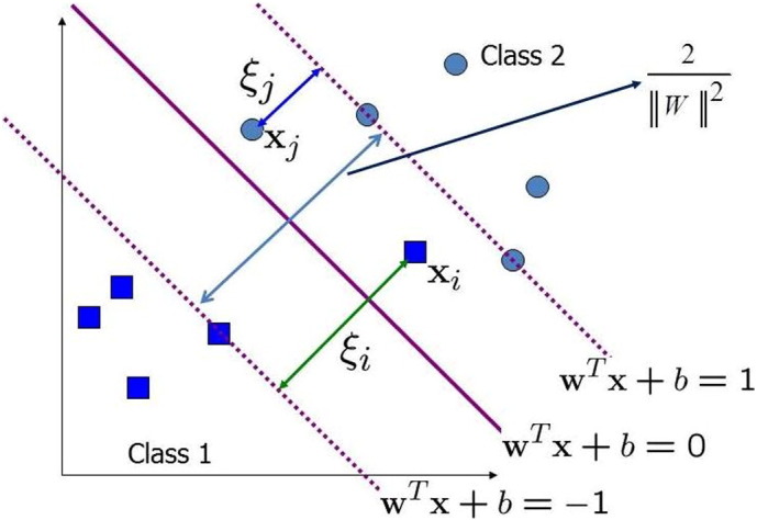
Maximum margin hyperplanes for SVM divides the plane into two classes.

By introducing Lagrange multipliers α_i (i = 1, 2, …, n) for the constraint, the primal problem becomes a task of finding the saddle point of Lagrange. Thus, the dual problem becomes:

$$\begin{array}{ll}maxL\left(\alpha \right)=\hfill & {\displaystyle \sum _{i=1}^n{\alpha }_i}-\frac{1}{2}{\displaystyle \sum _{\mathit{ij}}^n{\alpha }_i{\alpha }_j{y}_i}{y}_j\left(x_i\cdot x_j\right)\hfill \\ \text{subject}\mathrm{to}\hfill & {\displaystyle \sum _{i=1}^n{\alpha }_i}{y}_i=0\hfill \\ \hfill & {\alpha }_i\ge 0.\hfill \end{array}$$ (12)

By applying the Karush–Kuhn–Tucker (KKT) conditions, the following relationship holds α_i[y_i(Wx_i + b) − 1]. If a_i > 0, the corresponding data points are called support vectors (SVs). Hence, the optimal solution for the normal vector is given by $W*={\displaystyle \sum _{i=1}^N{\alpha }_i}{y}_i{x}_i$. Here N is the number of SVs. By choosing any SVs (x_k, y_k), we can obtain b * = y_k − W * x_k.

After (W*, b*) is determined, the discrimination function can be given by

$$f\left(x\right)=\text{sgn}\left({\displaystyle \sum _{i=1}^N{\alpha }_i}{y}_i\left(x_i\cdot x_j\right)+b*\right)$$ (13)

where sign (.) is the sign function.

In case of nonlinearly separable data, SVM has to map the data from the input space into a higher-dimensional feature space, where the classes can then be separated by a hyperplane. The function that performs this mapping is called a kernel function. In SVM the following four basic Kernel functions are used [35]:

• 1.Linear : K(X_i, X_j) = X_i^TX_j
• 2.$\mathit{Polynomial}:K\left(X_i,X_j\right)={\left(\gamma {X^T}_i,X_j+r\right)}^d,\gamma >0$
• 3.Radial basis function (RBF) : K(X_i, X_j) = exp (− γ‖X_i − X_j‖)² , γ > 0
• 4.$\mathit{Sigmoid}:K\left(X_i,X_j\right):tanh\left(\gamma {X_i}^T,X_j+r\right)$

where r, d and γ is a kernel parameter.

For nonlinearly separable data, SVM requires the solution of the following optimization problem:

$$\begin{array}{ll}\text{minimize}\hfill & \frac{1}{2}{‖W^T‖}^2+C{{\sum }_{i=1}}^n{\xi }_i\hfill \\ \text{subject}\mathrm{to}:\hfill & Y_i\left(W^T{X}_i+b\right)\ge 1-{\xi }_i\hfill \\ \hfill & {\xi }_i\ge 0\hfill \end{array}$$ (14)

where ξ_i ≥ 0 are slack variables that allow the elements of the training dataset to be at the margin or to be misclassified [36]. More detailed information on SVM can be found elsewhere [32], [37].

2.5. Naïve Bayes classifier

Naïve Bayes is one of the most efficient and effective inductive learning algorithms for machine learning and data mining, based on applying Bayes theorem with strong independence assumption [38], [39], [40]. After feature selection, Naïve Bayes classifier is built, which is used to classify a new test sample with features (gene) values E₁, E₂, …, E_n. Bayesian network classifier computes the posterior probability that the sample belongs to class H by using the Bayes theorem for multiple evidences as follows [1], [41], [42]:

$$P\left(H|E_1,E_2,E_3,\dots ,E_n\right)=\frac{P\left(E_1,E_2,E_3,\dots ,E_n|H\right)\times P\left(H\right)}{P\left(E_1,E_2,E_3,\dots ,E_n\right)}.$$ (15)

If the assumption of class-conditional independence among attributes is imposed, the following Naïve Bayes classifier can be obtained [15]:

$$P\left(H|E_1,E_2,E_3,\dots ,E_n\right)=\frac{P\left(E_1|H\right)\times P\left(E_2|H\right)\times \dots P\left(E_n|H\right)\times P\left(H\right)}{P\left(E_1,E_2,E_3,\dots ,E_n\right)}.$$ (16)

Since P(E₁, E₂, E₃, … , E_n) is a common factor for a certain sample, it can be ignored in the classification process. In addition, since the attribute variables are continuous in microarray data analysis, the probability density value f(E_i | H) can be used to replace the probability value P(E_i | H). The class-conditional probability density f(.| H) for each attribute and the prior P(H) can be obtained from the learning process. For the estimation of f(.| H) the nonparametric kernel density estimation method is used [13], [40], [43]. As a result, the general Bayesian classifier given by Eq. (15) can be simplified as the Naïve Bayes classifier given by Eq. (17). Fig. 3 shows the simplified form of a Bayesian classifier as the Naïve Bayes classifier [44].

$$H^{\mathit{\prime }}\mathit{=}arg\underset{H\in \omega }{max}P\left(H\right){\displaystyle \prod _{i\mathit{=}1}^{n}f\left(E_i|H\right)}$$ (17)

Fig. 3.

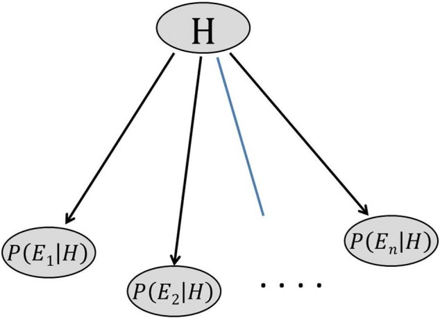
Naïve Bayes classifier.

3. Experiential setup

To evaluate the performance of the proposed feature selection approach for SVM and NB classifiers five publicly available microarray datasets, i.e. colon cancer [45], acute leukemia [46], prostate cancer [47], lung cancer-II [48], and high-grade glioma data [49] are taken. These datasets have been widely used to benchmark for the performance of gene selection methods in bioinformatics field. These datasets is downloaded from Kent ridge an online repository of high-dimensional biomedical datasets (http://datam.i2r.astar.edu.sg/datasets/krbd/index.html). Table 1 shows the five datasets with their properties.

Table 1.

Summary of five high dimensional biomedical microarray datasets (Kent ridge online repository).

Dataset	No. of classes	No. of features	Class balance +/−	No. of samples	Short description
Colon cancer [45]	2	2000	(22/40)	62	Data collect from colon cancer patient: tumor biopsies showing tumor negative and normal positive biopsies are from health parts of colons of the same patients.
Acute leukemia [46]	2	7129	(47/25)	72	Data collected from bone marrow samples: distinction is between Acute Myeloid Leukemia (AML) and Acute Lymphoblastic Leukemia (ALL) without previous knowledge of these classes.
Prostate tumor [47]	2	12,600	(50/52)	102	Data from prostate tumor samples where by the non-tumor (normal) prostate sample sand tumor samples (cancer) are identified.
High-grade glioma [49]	2	12,625	(28/22)	50	Data collected from brain tumor samples: distinction is between glioblastomas and anaplastic oligodendrogliomas.
Lung cancer II [48]	2	12,533	(31/150)	181	Data collected from tissue samples; classification between Malignant Pleural Mesothelioma (MPM) and Adenocarcinoma (ADCA) of the lung.

These datasets are preprocessed by setting thresholds and log-transformation on the original data. After preprocessing the data, it is divided into training and test set, further independent component analysis is performed to reduce the dimensionality of train data. For ICA, the FastICA algorithm software package for Matlab (R2010a) is applied it can be obtained from [53]. Then fuzzy feature selection technique is used for finding a small number of genes in independent component feature vectors. Codes for fuzzy feature selection are freely available on internet [54].

In this study, we tested the performance of the proposed fuzzy ICA algorithm by comparing it with most well-known standard extraction algorithms principal component analysis (PCA) [50].We compared the performance of each gene selection approach based on two parameters: the classification accuracy and the number of predicted genes that have been used for cancer classification. Classification accuracy is the overall precision of the classifier and is calculated as the sum of correct cancer classifications divided by the total number of classifications:

$$\text{Classification}\text{accuracy}\mathit{=}\frac{\mathrm{CC}}{\mathrm{N}}\times 100$$

where N is the total number of the instances in the initial microarray dataset and CC refers to correct classified instances. From early stage of the SVM, most of the researchers have used the linear, polynomial and RBF kernels for classification problems. From these kernels polynomial and RBF are the nonlinear kernel and cancer classification using microarray dataset is a nonlinear classification task [51], [52]. Nahar et al. observed from their experiment out of nine microarray datasets that the polynomial kernel is a first choice for microarray classification. Therefore, we used polynomial kernel for SVM classifier with parameter gamma = 1, d = 3 and value of 1 is used for the complexity constant parameter C and the random number of seed parameter W. In addition, we apply leave-one-out cross-validation (LOOCV) in order to evaluate the performance of our proposed algorithm with SVM and NB classifiers. We implement SVM, NB using the MATLAB software. Furthermore, in order to make experiments more statistically valid, we conduct each experiment 30 times on each dataset. In addition, average results and variance of the classification accuracies of the 30 independent runs are calculated in order to evaluate the performance of our proposed algorithm.

4. Experimental result

To check the performance of the proposed approach with SVM and NB classifiers, the above mentioned combination has been applied on the five DNA microarray gene expression datasets. Since all data samples in the five datasets have already been assigned to a training set or test set. The training dataset is used to do gene selection and then built the model for classification of the test dataset to evaluate the performances of alternative classifiers. To show the efficiency and feasibility of our proposed method, the results of the other three gene selection methods for the same classifier are also listed in Table 2, Table 3, Table 4, Table 5, Table 6 for comparison. In method 1, the microarray data are classified by SVM directly with all features. In the method 2, all the features are extracted by principle component analysis for SVM classification and the same is applied for method 3 except using ICA for feature extraction. Method 4 is similar to our proposed method where PCA is used with FBFE for SVM classification and in method 5 ICA with FBFE. The classification for pure Naïve Bayes classifier was not included due to its extremely time-consuming computations. In method 1 of NB classification PCA was used for feature extraction, in second ICA was used with NB. In methods 3 and 4 PCA and ICA were used with FBFE for NB classification respectively.

Table 2.

Classification result with colon cancer data.

S. no.	Classifier	Method	Mean accuracy	Variance
1.	SVM	SVM	88.19	0.061
2.	PCA + SVM	75.15	0.053
3.	ICA + SVM	79.19	0.052
4.	PCA + FBFE + SVM	83.34	0.032
5.	ICA + FBFE + SVM	90.09	0.026
1.	NB	PCA + NB	76.58	0.074
2.	ICA + NB	80.81	0.051
3.	PCA + FBFE + NB	82.65	0.032
4.	ICA + FBFE + NB	85.46	0.012

Table 3.

Classification result with acute leukemia data.

S. no.	Classifier	Method	Mean accuracy	Variance
1.	SVM	SVM	92.21	0.071
2.	PCA + SVM	76.67	0.054
3.	ICA + SVM	88.23	0.039
4.	PCA + FBFE + SVM	91.23	0.03
5.	ICA + FBFE + SVM	94.20	0.013
1.	NB	PCA + NB	68.23	0.053
2.	ICA + NB	86.21	0.051
3.	PCA + FBFE + NB	91.42	0.026
4.	ICA + FBFE + NB	95.12	0.023

Table 4.

Classification result with prostate tumor data.

S. no.	Classifier	Method	Mean accuracy	Variance
1.	SVM	SVM	78.43	0.102
2.	PCA + SVM	75.43	0.101
3.	ICA + SVM	80.45	0.092
4.	PCA + FBFE + SVM	83.23	0.076
5.	ICA + FBFE + SVM	88.12	0.043
1.	NB	PCA + NB	73.23	0.092
2.	ICA + NB	79.23	0.083
3.	PCA + FBFE + NB	83.22	0.052
4.	ICA + FBFE + NB	84.12	0.031

Table 5.

Classification result with high-grade glioma data.

S. no.	Classifier	Method	Mean accuracy	Variance
1.	SVM	SVM	69.23	0.067
2.	PCA + SVM	69.72	0.042
3.	ICA + SVM	70.21	0.043
4.	PCA + FBFE + SVM	73.32	0.047
5.	ICA + FBFE + SVM	79.21	0.041
1.	NB	PCA + NB	69.78	0.032
2.	ICA + NB	70.20	0.041
3.	PCA + FBFE + NB	74.32	0.021
4.	ICA + FBFE + NB	76.23	0.020

Table 6.

Classification result with lung cancer II data.

S. no.	Classifier	Method	Mean accuracy	Variance
1.	SVM	SVM	76.21	0.074
2.	PCA + SVM	75.23	0.081
3.	ICA + SVM	80.12	0.091
4.	PCA + FBFE + SVM	85.21	0.062
5.	ICA + FBFE + SVM	91.23	0.024
1.	NB	PCA + NB	80.54	0.061
2.	ICA +  NB	86.52	0.082
3.	PCA + FBFE + NB	91.32	0.034
4.	ICA + FBFE + NB	95.42	0.011

It can be seen from Table 2, Table 3, Table 4, Table 5, Table 6 that both FBFE + PCA and FBFE + ICA perform better than PCA and ICA in microarray data analysis, which demonstrates the effectiveness of the proposed approach. As for the comparison between the former two classification rules, FBFE + ICA perform obviously better than FBFE + PCA in terms of classification accuracy for both the classifier. It is clear that the classification accuracy of classifiers with our proposed method compared to other three gene selection methods with same classifiers is more accurate, feasible and reduces the variation of classification performance. Therefore, the proposed approach improves the classification performance of both the classifiers for microarray data. From the accuracy table of 2–6 different datasets, the performance of the proposed method for the high-grade glioma data, in contrast to the other 4 used datasets is low, because there is no method which could be applied universally to all the datasets to classify with maximum accuracy, since the properties of every datasets are different.

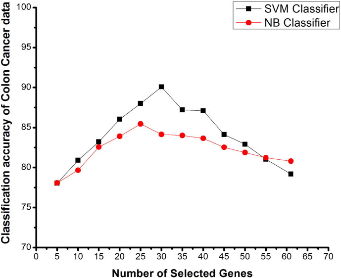
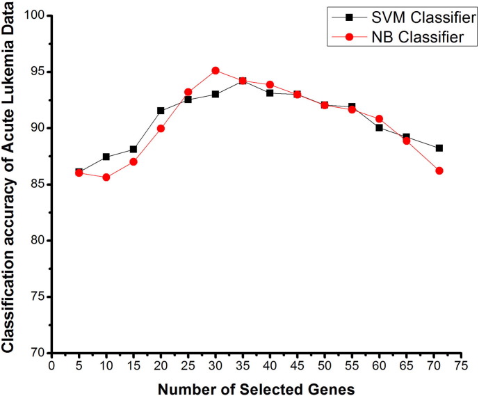
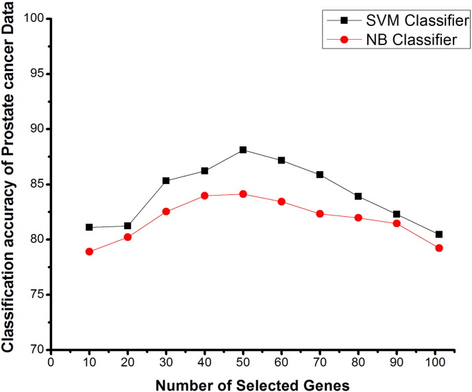
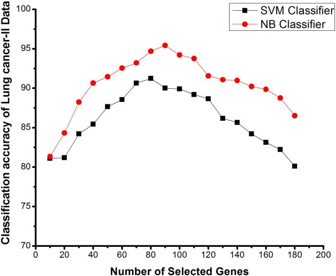
Since a small number of features are not enough for classification, while a large number of features may add noise and cause over fitting, fuzzy based backward elimination method is used for removing inappropriate genes from the independent component feature vector and the termination criterion in our method is based on the classification accuracy rate of the classifier. Since features with higher fuzzy entropy are less relevant to our classification goal, we eliminate the feature which has the highest fuzzy entropy. If the classification rate does not decrease, then the above step is repeated until all “inappropriate” features are removed. Finally, the features that remained were used for classification and then the mean classification accuracies and variances were computed. In order to study the behavior of a proposed feature selection approach, it is applied to the colon, leukemia, prostate, high-grade glioma and lung cancer II dataset for SVM and NB classification, a graph is plotted between the number of features and classification accuracy rates. Fig. 4, Fig. 5, Fig. 6, Fig. 7, Fig. 8 show the variation of the number of selected genes V/s classification accuracy, using SVM and NB classifiers.

Fig. 4.

Number of selected genes V/s classification accuracy using SVM and NB classifiers on colon cancer data, based on proposed method.

Fig. 5.

Number of selected genes V/s classification accuracy using SVM and NB classifiers on acute leukemia data based on proposed method.

Fig. 6.

Number of selected genes V/s classification accuracy using SVM and NB classifiers on prostate tumor data, based on proposed feature method.

Fig. 7.

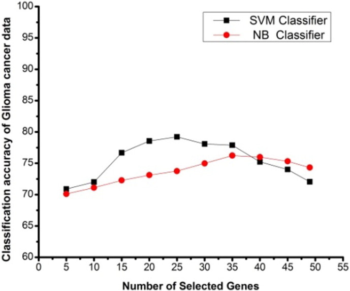
Number of selected genes V/s classification accuracy using SVM and NB classifiers on high-grade glioma data, based on proposed method.

Fig. 8.

Number of selected genes V/s classification accuracy using SVM and NB classifiers on a lung cancer II data, based on proposed method.

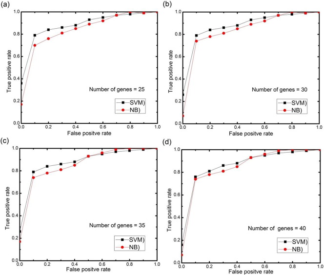
The colon cancer dataset consists of 62 samples with 2000 (genes) features of two classes. Fig. 4 shows the graph between the number of selected genes and the classification accuracy, using SVM and NB classifiers for colon cancer data based on the proposed gene selection method. Here by reducing the gene, the mean classification accuracy was enhanced significantly. The classification accuracy with all 61 selected genes of training set was 79.19%. The mean improvement in classification accuracy was verified by eliminating 5 genes, each time from training sets. Interestingly, the best mean accuracy with the proposed method was found to be 90.09% for 30 selected features and 85.46% for 25 selected genes with SVM and NB classifiers respectively. There is a sudden increase in the classification accuracy with the elimination of the genes from 61 to 30 for SVM classification, further reduction in the genes again decreases the classification accuracy. Moreover, as can be seen from Fig. 4, the results were improving almost all the time, when genes were reduced and finally best results were obtained, using only 30 and 25 genes from the training dataset using SVM and NB classifiers respectively. This also suggests a significant reduction in computational cost and simplifies the model a lot.

Acute leukemia dataset consists of 72 samples with 7129 genes of two classes. Fig. 5 shows the results of classification accuracy with the number of selected genes for leukemia dataset. As shown in Table 3, with this dataset using SVM and NB classifiers with ICA feature vector, the highest mean accuracy obtained was 88.23% and 86.21%. When FBFE approach is used in independent component feature vector, one managed to get 94.2% and 95.12% mean classification accuracies for SVM and NB classifiers respectively. Fuzzy backward feature elimination (FBFE) approach is used to eliminate the irrelevant and correlated genes from the independent components. The peak of the graphs shows that here, 35 genes for SVM and 30 genes for NB were used for best classification accuracy.

Fig. 6 shows the graph for the classification accuracy of the prostate cancer dataset with a number of selected genes using FBFE and ICA approach with SVM and NB classifiers. The peak of the graph shows the maximum classification accuracy of this dataset. Interestingly, for both SVM and NB classifiers the selection of 50 genes gives the highest mean classification accuracy. Classification accuracy of this dataset with SVM classifier is more as compared with the NB classifier with the same number of selected genes. Though the classification accuracy with ICA + SVM and ICA + NB as shown in the Table 4 was 80.45% and 79.23%, the mean classification accuracy for SVM and NB classifiers is 88.12% and 84.12% respectively with the proposed approach. These results clearly show that the FBFE approach with ICA performs better than the other existing methods.

High-grade glioma dataset consist of 50 samples with 12,625 genes of two classes. From this dataset 49 genes are extracted by FastICA from the training set. Fig. 7 shows the classification accuracy graph of high-grade glioma data by the elimination of the genes with FBFE, using SVM and NB classifiers. From Fig. 5 it is clear that, by eliminating 5 genes here for this data, there is a difference of 10 genes between the SVM and NB classification for the highest mean classification accuracy which is more as compared with the other selections. It can be seen from the graph that the highest mean accuracies for glioma dataset was found with 25 and 35 (with the difference of 10 genes) selected genes for SVM and NB classifications respectively. There is a gradual increase in the classification accuracy with the elimination of genes for both SVM and NB classifications. The values of mean classification accuracy with the proposed method for SVM and NB classifiers are 79.21% and 76.23%, respectively, which is very low as compared to the accuracies of the other datasets.

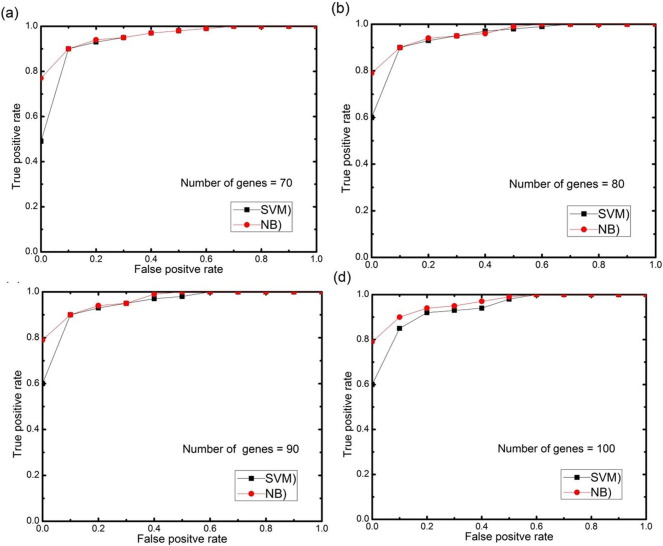
In lung cancer-II dataset there were 181 samples with 12,533 genes. Fig. 8 clearly shows the difference between the classification accuracies of this dataset using SVM and NB classifiers. It is clear from the accuracy graph that classification accuracy of NB is more as compared to the accuracy of the SVM classifier with our proposed method. A sudden increase in the mean classification accuracy is seen with the elimination of the genes using ICA and FBFE with SVM and NB classifiers. The highest mean accuracy obtained was 80.12% and 86.52% with an ICA feature vector as shown in Table 6 using SVM and NB classifiers. With our proposed method, the mean accuracy obtained is 91.23% with 80 genes and 95.42% with 90 genes for SVM and NB classification, which shows that the FBFE approach with ICA performs better than the other existing methods.

Fig. 9, Fig. 10 show the graph of the average error rate of SVM and NB classifiers respectively, for the five datasets with different gene selection methods. It is clearly shown in the figure that ICA + FBFE with SVM and NB classifiers performs better than the other gene selection methods because of the reduced error rate, which shows the significance of the proposed method with the other existing methods. It is evident from the graph that when genes are selected, based on FBFE from PCA then the percentage error rate is minimized, which shows that FBFE with PCA performs better than PCA method with SVM and NB classifiers.

Fig. 9.

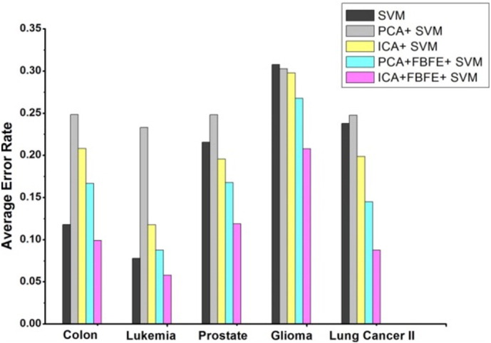
Average error rate of SVM classifier for the five datasets with different gene selection methods.

Fig. 10.

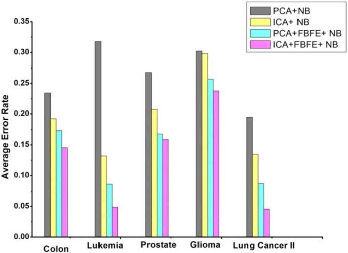
Average error rate of NB classifier for the five datasets with different gene selection methods.

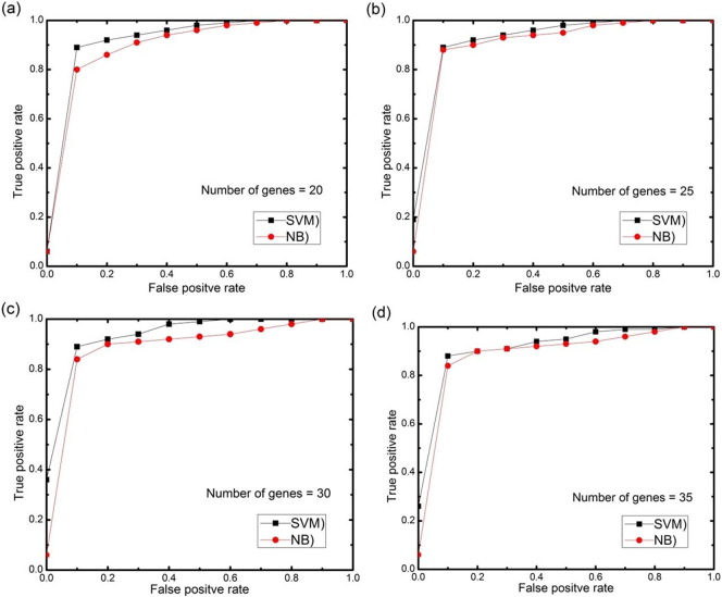
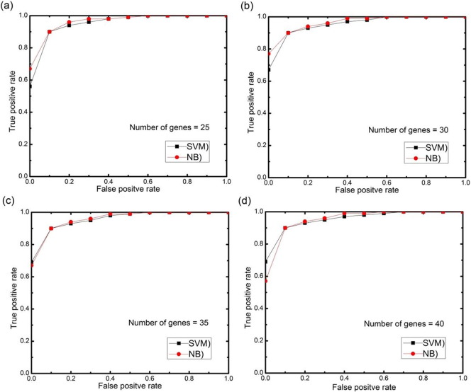
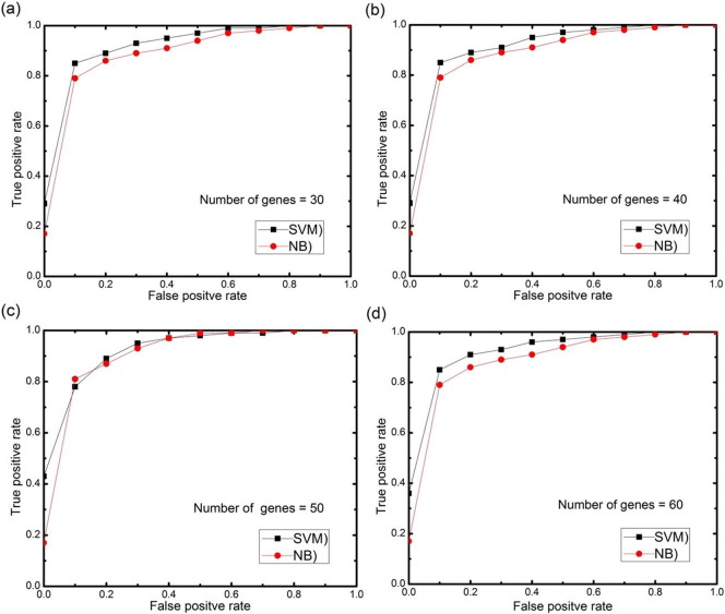
For further analysis, AUC (area under the ROC curve) curves obtained on the test set using different numbers of selected features genes (features) with 0.5 threshold value for each datasets are depicted in Fig. 11, Fig. 12, Fig. 13, Fig. 14, Fig. 15. The highest AUC values for each datasets with the number of selected genes that gives these highest values are shown in Table 7. From Fig. 11, Fig. 12, Fig. 13, Fig. 14, Fig. 15 we can see that, how the AUC changes with different number of genes. For the colon data (Fig. 11a–d), the highest value of AUC is 0.91 with 30 genes for SVM classifier and 0.85 with 25 genes for NB classifier. For acute leukemia dataset, as the value of selected gene set increases from 30 to 35, AUC also increases from 0.93 to 0.94 for SVM classifier, on the other hand with the same increase in selected gene set for NB classifier, AUC decreases from 0.95 to 0.94. Resultantly it is concluded that 35 genes are best for SVM classifier and 30 are best for NB classifier. For prostate dataset, highest value of AUC obtained with 50 numbers of selected genes for both the classifiers. For high grade glioma data, 25 gene set gives the highest value of AUC because further increase in gene, decreases the value of AUC for SVM classifier and for NB classifier 35 selected genes gives the highest value of AUC. From Fig. 15a–d for lung cancer data it is clear that with 80 selected gene set, the highest AUC value is found to be 0.91 for SVM classifier and with 90 selected genes the highest AUC value is 0.95 for NB classifier. It is immediately apparent from these results that, with this particular setup, we can find the number of selected genes that gives the best classification accuracy.

Fig. 11.

(a–d) AUC curves on the test set for both the classifiers with different numbers of selected genes using proposed approach for colon cancer data.

Fig. 12.

(a–d) AUC curves on the test set for both the classifiers with different numbers of selected genes using proposed approach for acute leukemia data.

Fig. 13.

(a–d) AUC curves on the test set for both the classifiers with different numbers of selected genes using proposed approach for prostate tumor data.

Fig. 14.

(a–d) AUC curves on the test set for both the classifiers with different numbers of selected genes using proposed approach for high-grade glioma data.

Fig. 15.

(a–d) AUC curves on the test set for both the classifiers with different numbers of selected genes using proposed approach for lung cancer II data.

Table 7.

Highest AUC values for both the classifiers with best values of selected features using proposed approach for different datasets.

S. no.	Datasets	SVM classifier		NB classifier
Highest area under the ROC curve	Best values of selected features	Highest area under the ROC curve	Best values of selected features
1.	Colon cancer	0.9126	30	0.8566	25
2.	Acute leukemia	0.9468	35	0.9536	30
3.	Prostate tumor	0.8857	50	0.8427	50
4.	High-grade glioma	0.7933	25	0.7644	35
5.	Lung cancer II	0.9144	80	0.9588	90

Therefore, with this fuzzy backward feature selection procedure, discarding redundant, noise-corrupted or unimportant features, we can reduce the dimensionality of any type of microarray data to speed up the classification process, increase the accuracy rate of the classification and making the computational expenses affordable.

5. Conclusion

This paper presents a fuzzy backward feature elimination approach in ICA feature vector for SVM and NB classifications of microarray data where the methodologies involve dimension reduction of microarray data using ICA, followed by the feature selection using FBFE. The approach was tested by classifying five datasets. ROC shows the best subset of genes, which gives the highest classification accuracy for both the classifier of different datasets using proposed approach. The experimental results show that our combination of gene selection methods of an existing algorithm together with SVM and NB classifiers is giving better results as compared to other existing approaches. Our experimental results on five microarray datasets demonstrate the effectiveness of the proposed approach in improving the classification performance of SVM and NB classifiers in microarray data analysis. It is observed that the proposed method can obtain better classification accuracy with a smaller number of selected genes than the other existing methods, so our proposed method is effective and efficient for SVM and NB classifiers.

Conflict of interest

The authors declare no conflict of interest.

References

- 1.Fan L., Poh K.-L., Zhou P. A sequential feature extraction approach for Naïve Bayes classification of microarray data. Expert Syst. Appl. 2009;36:9919–9923. [Google Scholar]
- 2.Vilda P.G., Díaz F., Martínez R., Malutan R., Rodellar V., Puntonet C.G. Independent Component Analysis and Blind Signal Separation. Springer; 2006. Robust preprocessing of gene expression microarrays for independent component analysis; pp. 714–721. [Google Scholar]
- 3.Zheng C.-H., Huang D.-S., Shang L. Feature selection in independent component subspace for microarray data classification. Neurocomputing. 2006;69:2407–2410. [Google Scholar]
- 4.Peng Y. A novel ensemble machine learning for robust microarray data classification. Comput. Biol. Med. 2006;36:553–573. doi: 10.1016/j.compbiomed.2005.04.001. [DOI] [PubMed] [Google Scholar]
- 5.Hammer B., Villmann T. ESANN. Citeseer; 2003. Mathematical aspects of neural networks; pp. 59–72. [Google Scholar]
- 6.Du D., Li K., Li X., Fei M. A novel forward gene selection algorithm for microarray data. Neurocomputing. 2014;133:446–458. [Google Scholar]
- 7.Gutkin M. Tel-Aviv University; 2008. Feature Selection Methods for Classification of Gene Expression Profiles. [Google Scholar]
- 8.Tang E.K., Suganthan P.N., Yao X. Computational Intelligence in Bioinformatics and Computational Biology, 2005. CIBCB'05. Proceedings of the 2005 IEEE Symposium on, IEEE. 2005. Feature selection for microarray data using least squares svm and particle swarm optimization; pp. 1–8. [Google Scholar]
- 9.Bartenhagen C., Klein H.-U., Ruckert C., Jiang X., Dugas M. Comparative study of unsupervised dimension reduction techniques for the visualization of microarray gene expression data. BMC Bioinf. 2010;11:567. doi: 10.1186/1471-2105-11-567. [DOI] [PMC free article] [PubMed] [Google Scholar]
- 10.Frigyesi A., Veerla S., Lindgren D., Höglund M. Independent component analysis reveals new and biologically significant structures in micro array data. BMC Bioinf. 2006;7:290. doi: 10.1186/1471-2105-7-290. [DOI] [PMC free article] [PubMed] [Google Scholar]
- 11.Zheng C.-H., Huang D.-S., Kong X.-Z., Zhao X.-M. Gene expression data classification using consensus independent component analysis. Genomics Proteomics Bioinformatics. 2008;6:74–82. doi: 10.1016/S1672-0229(08)60022-4. [DOI] [PMC free article] [PubMed] [Google Scholar]
- 12.Mohan A., Rao M.D., Sunderrajan S., Pennathur G. Automatic classification of protein structures using physicochemical parameters. Interdiscip. Sci.: Comput. Life Sci. 2014;6:176–186. doi: 10.1007/s12539-013-0199-0. [DOI] [PubMed] [Google Scholar]
- 13.Fan L., Poh K.-L., Zhou P. Partition-conditional ICA for Bayesian classification of microarray data. Expert Syst. Appl. 2010;37:8188–8192. [Google Scholar]
- 14.Patil T.R., Sherekar M. Performance analysis of Naive Bayes and J48 classification algorithm for data classification. Int. J. Comput. Sci. Appl. 2013;6:256–261. [Google Scholar]
- 15.Zhang H. Exploring conditions for the optimality of naive Bayes. Int. J. Pattern Recognit. Artif. Intell. 2005;19:183–198. [Google Scholar]
- 16.Statnikov A., Henaff M., Narendra V., Konganti K., Li Z., Yang L., Pei Z., Blaser M.J., Aliferis C.F., Alekseyenko A.V. A comprehensive evaluation of multicategory classification methods for microbiomic data. Microbiome. 2013;1:11. doi: 10.1186/2049-2618-1-11. [DOI] [PMC free article] [PubMed] [Google Scholar]
- 17.Chakraborty S., Guo R. A Bayesian hybrid Huberized support vector machine and its applications in high-dimensional medical data. Comput. Stat. Data Anal. 2011;55:1342–1356. [Google Scholar]
- 18.Hyvärinen A., Oja E. A fast fixed-point algorithm for independent component analysis. Neural Comput. 1997;9:1483–1492. [Google Scholar]
- 19.Naik G.R., Kumar D.K. An overview of independent component analysis and its applications. Informatica. 2011;35:63–81. [Google Scholar]
- 20.Engreitz J.M., Daigle B.J., Marshall J.J., Altman R.B. Independent component analysis: mining microarray data for fundamental human gene expression modules. J. Biomed. Inform. 2010;43:932–944. doi: 10.1016/j.jbi.2010.07.001. [DOI] [PMC free article] [PubMed] [Google Scholar]
- 21.Kong W., Vanderburg C.R., Gunshin H., Rogers J.T., Huang X. A review of independent component analysis application to microarray gene expression data. Biotechniques. 2008;45:501. doi: 10.2144/000112950. [DOI] [PMC free article] [PubMed] [Google Scholar]
- 22.Hyvärinen A., Karhunen J., Oja E. John Wiley & Sons; 2004. Independent Component Analysis. [Google Scholar]
- 23.Capobianco E. 2004. Exploration and Reduction of High Dimensional Spaces With Independent Component Analysis. [Google Scholar]
- 24.Luukka P. Feature selection using fuzzy entropy measures with similarity classifier. Expert Syst. Appl. 2011;38:4600–4607. [Google Scholar]
- 25.Parkash O., Gandhi C. Applications of trigonometric measures of fuzzy entropy to geometry. Int. J. Math. Comput. Sci. 2010;6:76–79. [Google Scholar]
- 26.Cesar I. 2012. Feature Selection Using Fuzzy Entropy Measures With Yu's Similarity Measure. [Google Scholar]
- 27.Lee H.-M., Chen C.-M., Chen J.-M., Jou Y.-L. An efficient fuzzy classifier with feature selection based on fuzzy entropy. IEEE Trans. Syst. Man Cybern. B Cybern. 2001;31:426–432. doi: 10.1109/3477.931536. [DOI] [PubMed] [Google Scholar]
- 28.Pochet N., De Smet F., Suykens J.A., De Moor B.L. Systematic benchmarking of microarray data classification: assessing the role of non-linearity and dimensionality reduction. Bioinformatics. 2004;20:3185–3195. doi: 10.1093/bioinformatics/bth383. [DOI] [PubMed] [Google Scholar]
- 29.Cortes C., Vapnik V. Support-vector networks. Mach. Learn. 1995;20:273–297. [Google Scholar]
- 30.Vapnik V. Wiley; New York: 1998. Statistical Learning Theory. [Google Scholar]
- 31.Mukherjee S., Vapnik V. Vol. 170. Center for Biological and Computational Learning, Department of Brain and Cognitive Sciences, MIT. CBCL; 1999. Support Vector Method for Multivariate Density Estimation. [Google Scholar]
- 32.Boser B.E., Guyon I.M., Vapnik V.N. Proceedings of the Fifth Annual Workshop on Computational Learning Theory, ACM. 1992. A training algorithm for optimal margin classifiers; pp. 144–152. [Google Scholar]
- 33.Jan J., Kilián P., Provazník I. Technical University Brno Press; 1996. Analysis of Biomedical Signals and Images. [Google Scholar]
- 34.Kostka P.S., Tkacz E.J. Engineering in Medicine and Biology Society, 2008. EMBS 2008, 30th Annual International Conference of the IEEE. IEEE; 2008. Feature extraction based on time-frequency and independent component analysis for improvement of separation ability in atrial fibrillation detector; pp. 2960–2963. [DOI] [PubMed] [Google Scholar]
- 35.Hsu C.-C., Chen M.-C., Chen L.-S. Integrating independent component analysis and support vector machine for multivariate process monitoring. Comput. Ind. Eng. 2010;59:145–156. [Google Scholar]
- 36.DURGESH K.S., Lekha B. Data classification using support vector machine. J.Theor. Appl. Inf. Technol. 2010;12:1–7. [Google Scholar]
- 37.Huang H.-L., Chang F.-L. ESVM: evolutionary support vector machine for automatic feature selection and classification of microarray data. Biosystems. 2007;90:516–528. doi: 10.1016/j.biosystems.2006.12.003. [DOI] [PubMed] [Google Scholar]
- 38.Langley P., Iba W., Thompson K. AAAI. 1992. An analysis of Bayesian classifiers; pp. 223–228. [Google Scholar]
- 39.Friedman N., Geiger D., Goldszmidt M. Bayesian network classifiers. Mach. Learn. 1997;29:131–163. [Google Scholar]
- 40.John G.H., Langley P. Proceedings of the Eleventh conference on Uncertainty in artificial intelligence. Morgan Kaufmann Publishers Inc.; 1995. Estimating continuous distributions in Bayesian classifiers; pp. 338–345. [Google Scholar]
- 41.Chen J., Huang H., Tian S., Qu Y. Feature selection for text classification with Naïve Bayes. Expert Syst. Appl. 2009;36:5432–5435. [Google Scholar]
- 42.Sandberg R., Winberg G., Bränden C.-I., Kaske A., Ernberg I., Cöster J. Capturing whole-genome characteristics in short sequences using a naive Bayesian classifier. Genome Res. 2001;11:1404–1409. doi: 10.1101/gr.186401. [DOI] [PMC free article] [PubMed] [Google Scholar]
- 43.De Campos L.M., Cano A., Castellano J.G., Moral S. 2011 11th International Conference on Intelligent Systems Design and Applications (ISDA), IEEE. 2011. Bayesian networks classifiers for gene-expression data; pp. 1200–1206. [Google Scholar]
- 44.Ji Y., Tsui K.-W., Kim K. Technical Report. Department of Biostatistics and Medical Informatics, University of Wisconsin-Madison; 2002. A Bayesian classification method for treatments using microarray gene expression data. [Google Scholar]
- 45.Alon U., Barkai N., Notterman D.A., Gish K., Ybarra S., Mack D., Levine A.J. Broad patterns of gene expression revealed by clustering analysis of tumor and normal colon tissues probed by oligonucleotide arrays. Proc. Natl. Acad. Sci. 1999;96:6745–6750. doi: 10.1073/pnas.96.12.6745. [DOI] [PMC free article] [PubMed] [Google Scholar]
- 46.Golub T.R., Slonim D.K., Tamayo P., Huard C., Gaasenbeek M., Mesirov J.P., Coller H., Loh M.L., Downing J.R., Caligiuri M.A. Molecular classification of cancer: class discovery and class prediction by gene expression monitoring. Science. 1999;286:531–537. doi: 10.1126/science.286.5439.531. [DOI] [PubMed] [Google Scholar]
- 47.Singh D., Febbo P.G., Ross K., Jackson D.G., Manola J., Ladd C., Tamayo P., Renshaw A.A., D'Amico A.V., Richie J.P. Gene expression correlates of clinical prostate cancer behavior. Cancer Cell. 2002;1:203–209. doi: 10.1016/s1535-6108(02)00030-2. [DOI] [PubMed] [Google Scholar]
- 48.Gordon G.J., Jensen R.V., Hsiao L.-L., Gullans S.R., Blumenstock J.E., Ramaswamy S., Richards W.G., Sugarbaker D.J., Bueno R. Translation of microarray data into clinically relevant cancer diagnostic tests using gene expression ratios in lung cancer and mesothelioma. Cancer Res. 2002;62:4963–4967. [PubMed] [Google Scholar]
- 49.Nutt C.L., Mani D., Betensky R.A., Tamayo P., Cairncross J.G., Ladd C., Pohl U., Hartmann C., McLaughlin M.E., Batchelor T.T. Gene expression-based classification of malignant gliomas correlates better with survival than histological classification. Cancer Res. 2003;63:1602–1607. [PubMed] [Google Scholar]
- 50.Hira Z.M., Gillies D.F. 2015. A Review of Feature Selection and Feature Extraction Methods Applied on Microarray Data. [DOI] [PMC free article] [PubMed] [Google Scholar]
- 51.Nahar J., Ali S., Chen Y.-P.P. Microarray data classification using automatic SVM kernel selection. DNA Cell Biol. 2007;26:707–712. doi: 10.1089/dna.2007.0590. [DOI] [PubMed] [Google Scholar]
- 52.Aziz R., Srivastava N., Verma C.K. t-Independent component analysis for SVM classification of DNA — microarray data. Int. J. Bioinforma. Res. 2015;6:305–312. [Google Scholar]
- 53.http://research.ics.aalto.fi/ica/fastica/code/dlcode.shtml.
- 54.http://in.mathworks.com/matlabcentral/fileexchange/31366-feature-selection-using-fuzzyentropy-measures-and-similarity.