A Primer on Bayesian Decision Analysis With an Application to a Personalized Kidney Transplant Decision

Abstract

To provide personalized medicine, we not only must determine the treatments and other decisions most likely to be effective for a patient, but also consider the patient’s tradeoff between possible benefits of therapy versus possible loss of quality of life. There are numerous studies indicating that various treatments can negatively affect quality of life. Even if we have all information available for a given patient, it is an arduous task to amass the information to reach a decision that maximizes the utility of the decision to the patient. A clinical decision support system (CDSS) is a computer program, which is designed to assist healthcare professionals with decision making tasks. By utilizing emerging large datasets, we hold promise for developing CDSSs that can predict how treatments and other decisions can affect outcomes. However, we need to go beyond that; namely our CDSS needs to account for the extent to which these decisions can affect quality of life. This manuscript provides an introduction to developing CDSSs using Bayesian networks and influence diagrams. Such CDSSs are able to recommend decisions that maximize the expected utility of the predicted outcomes to the patient. By way of comparison, we examine the benefit and challenges of the Kidney Donor Risk Index (KDRI) as a decision support tool, and we discuss several difficulties with this index. Most importantly, the KDRI does not provide a measure of the expected quality of life if the kidney is accepted versus the expected quality of life if the patient stays on dialysis. Finally, we develop a schema for an influence diagram that models the kidney transplant decision, and show how the influence diagram approach can resolve these difficulties and provide the clinician and the potential transplant recipient with a valuable decision support tool.

Introduction

“Precision medicine is an emerging approach for disease treatment and prevention that takes into account individual variability in genes, environment, and lifestyle for each person.” [1]. To provide personalized medicine, we not only must take into account the patient’s clinical and genomic profiles to determine the treatments most likely to be effective, but also consider the patient’s tradeoff between possible benefits of therapy versus loss of quality of life. There are numerous studies indicating the treatments can negatively affect quality of life, and so can outcomes such as distant metastasis and loco-regional occurrence [2, 3, 4]. Even if we have all information available for a given patient, it is an arduous task to amass the information to reach a decision that maximizes the utility of the decision to the patient.

A clinical decision support system (CDSS) is a computer program, which is designed to assist healthcare professionals with decision making tasks, such as determining the diagnosis and treatment of a patient [5]. A CDSS provides the capability of integrating all patient information towards recommending a decision. There have been various hurdles to the development of CDSSs including lack of large-scale data [6]. However, we are now approaching the era of “big” data where abundant clinical and genomic data are becoming increasingly available. By utilizing these data, we hold promise for developing CDSSs that can predict how treatment options and other decisions can affect outcomes such as survival. Furthermore, our CDSSs should account for the extent to which these decisions can affect quality of life in order to recommend a decision. We provide an introduction to developing CDSSs using Bayesian networks and influence diagrams. Such CDSSs are able to recommend decisions that maximize the expected utility of the predicted outcomes to the patient.

A recent decision support tool for the kidney transplant decision is the Kidney Donor Risk Index (KDRI) [7]. We briefly review that index and point out difficulties with it. Most importantly, it does not provide a measure of the expected quality of life if the kidney is accepted versus the expected quality of life if the patient stays on dialysis. We then develop a schema for an influence diagram that models the kidney transplant decision, and show how the influence diagram approach can resolve these difficulties and provide the potential transplant recipient with a true decision support tool.

Bayesian Networks

A Bayesian network [8–11] is a graphical model for representing the probabilistic relationships among variables, which has been applied extensively to biomedical informatics [12–15]. Since Bayesian networks are an extension of Bayes’ Theorem, we start by reviewing Bayes’ Theorem.

Suppose Sam plans to marry, and to obtain a marriage license in the state in which he resides, one must take the blood test enzyme-linked immunosorbent assay (ELISA), which tests for the presence of human immunodeficiency virus (HIV). Sam takes the test and it comes back positive for HIV. How likely is it, that Sam is infected with HIV? Without knowing the accuracy of the test, Sam really has no way of knowing how probable it is that he is infected with HIV.

The data we ordinarily have on such tests are the true positive rate (sensitivity) and the true negative rate (specificity). The true positive rate is the number of people who both have the infection and test positive divided by the total number of people who have the infection. For example, to obtain this number for ELISA, 10,000 people who were known to be infected with HIV were identified. This was done using the Western Blot, which is the gold standard test for HIV. These people were then tested with ELISA, and 9990 tested positive. Therefore, the true positive rate is 0.999. The true negative rate is the number of people who both do not have the infection and test negative divided by the total number of people who do not have the infection. To obtain this number for ELISA, 10,000 nuns who denied risk factors for HIV infection were tested. Of these, 9980 tested negative using the ELISA test. Furthermore, the 20 positive-testing nuns tested negative using the Western Blot test. So, the true negative rate is 0.998, which means that the false positive rate (1-specificity) is 0.002. We therefore formulate the following random variables and subjective probabilities:

$$\begin{array}{c}P(\mathit{ELISA}=\mathit{positive}\mid \mathit{HIV}=\mathit{present})=.999\\ P(\mathit{ELISA}=\mathit{positive}\mid \mathit{HIV}=\mathit{absent})=\mathrm{.002.}\end{array}$$

It might seem that Sam almost certainly is infected with HIV, as the test is so accurate. However, notice that neither of the above probabilities are the probability of Sam being infected with HIV. Because we know that Sam tested positive on ELISA, that probability is

$$P(\mathit{HIV}=\mathit{present}\mid \mathit{ELISA}=\mathit{positive}).$$

We can compute this probability using Bayes' theorem if we know P(HIV = present) . Recall that Sam took the blood test simply because the state required it. He did not take it because he thought for any reason he was infected with HIV. So, the only other information we have about Sam is that he is a male in the state in which he resides. Therefore if 1 in 100,000 men in Sam's state is infected with HIV, we assign the following probability:

$$P(\mathit{HIV}=\mathit{present})=\mathrm{0.00001.}$$

We now employ Bayes' theorem to compute

$$\begin{array}{l}P(\mathit{present}\mid \mathit{positive})=\frac{P(\mathit{positive}\mid \mathit{present})P(\mathit{present})}{P(\mathit{positive}\mid \mathit{present})P(\mathit{present})+P(\mathit{positive}\mid \mathit{absent})P(\mathit{absent})}\\ =\frac{(0.999)(0.00001)}{(0.999)(0.00001)+(0.002)(0.99999)}\\ =\mathrm{0.00497.}\end{array}$$ (1)

Surprisingly, we are fairly confident that Sam is not infected with HIV. A probability such as P(HIV = present) is called a prior probability because it is the probability of some event prior to updating the probability of that event using new information. A probability such as P(HIV = present | ELISA = positive) is called a posterior probability because it is the probability of an event after its prior probability has been updated based on new information. In the previous example, the reason the posterior probability is small, even though the test is fairly accurate, is that the prior probability is extremely low.

As another example, suppose Mary and her husband have been trying to have a baby and she suspects she is pregnant. She takes a pregnancy test that has a true positive rate of 0.99 and a false positive rate of 0.02. Suppose further that 20% of all women who take this pregnancy test are indeed pregnant. Using Bayes' theorem we then have

$$\begin{array}{l}P(\mathit{present}\mid \mathit{positive})=\frac{P(\mathit{positive}\mid \mathit{present})P(\mathit{present})}{P(\mathit{positive}\mid \mathit{present})P(\mathit{present})+P(\mathit{positive}\mid \mathit{absent})P(\mathit{absent})}\\ =\frac{(0.99)(0.2)}{(0.99)(0.2)+(0.02)(0.8)}\\ =\mathrm{0.92523.}\end{array}$$

Even though Mary's test was less accurate than Sam's test, she probably is pregnant, whereas he probably is not infected with HIV. This is due to the prior information. There was a significant prior probability (0.2) that Mary was pregnant, because only women who suspect they are pregnant on other grounds take pregnancy tests. Sam, however, took his test because he wanted to get married. We had no prior information indicating he could be infected with HIV.

Figure 1 summarizes the information used in the application of Bayes Theorem in Equation 1. That figure is a two-variable Bayesian network. Notice that it represents the variables HIV and ELISA by nodes in a Directed Acyclic Graph (DAG) and the causal relationship between these variables with an edge from HIV to ELISA. That is, the presence of HIV has a causal effect on whether the test result is positive; so there is an edge from HIV to ELISA. Besides showing a DAG representing the causal relationships, Figure 1 shows the prior probability distribution of HIV and the conditional probability distribution of ELISA given each value of its parent HIV.

Figure 1.

A two-variable Bayesian network.

In general, a Bayesian network consist of a DAG, whose edges represent relationships among variables that are often (but not always) causal; the prior probability distribution of every variable that is a root in the DAG; and the conditional probability distribution of every non-root variable given each set of values of its parents. Figure 2 shows a Bayesian network modeling relationships among variables related to respiratory diseases. We often refer to the variables in a Bayesian network as nodes.

Figure 2.

A Bayesian network representing relationships among variables related to respiratory diseases.

Using a Bayesian network, we can determine probabilities of interest with a Bayesian network inference algorithm [8], which repeatedly performs computations similar to those in the application of Bayes Theorem in Equation 1. For example, using the Bayesian network in Figure 1, if a patient has a smoking history (H = yes), a positive chest X-ray (X = pos), and a positive computer tomogram (CT = pos), we can determine the probability of the patient having lung cancer (L = yes). That is, we can compute P(L = yes| H = yes, X = pos, CT = pos), which turns out to be 0.185. The prior probability of lung cancer in this model is 0.0064. So, the evidence has increased the probability of lung cancer substantially.

Recommending Decisions

After introducing decision analysis, we discuss influence diagrams and quality adjusted life expectancy.

Decision Analysis

Decision analysis is the discipline that formally analyzes decision alternatives, and recommends the alternative that maximizes the expected utility of the outcome to the decision maker. As an example, suppose you have $1000, and are considering buying stock X, whose current price is $10 per share. Your time horizon is one month, and you feel there is about a 0.6 probability X will be at $11 per share in one month, and there is a 0.4 probability it will be at $9 per share. Your decision alternatives are d1, which is to buy X, and d2, which is to do nothing. Figure 3 shows a decision tree representing this decision. In decision analysis, we compute the expected value of each alternative:

$$\begin{array}{l}E(d1)=0.6(\$1100)+0.4(\$900)\\ =\$1020\\ E(d2)=\$1000.\end{array}$$

Figure 3.

A simple decision tree representing the decision whether to buy stock X.

If you are an expected value maximizer, you would choose d1.

Influence Diagrams

Often a problem is too complex to represent it using a decision tree because the size of the decision tree model grows exponentially with the size of the problem. An influence diagram is a Bayesian network augmented with decision nodes, and can represent all the same problems as a decision tree. Its size grows linearly with the size of the problem. Figure 4 shows the previous example represented with an influence diagram.

Figure 4.

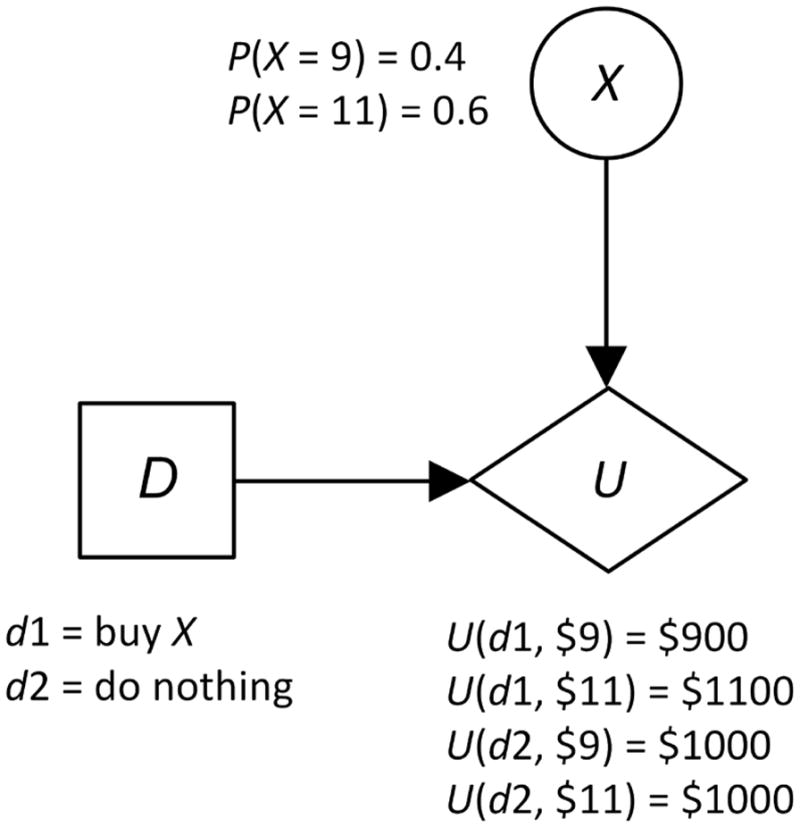
An influence diagram modeling the problem determined by the decision tree in Figure 3.

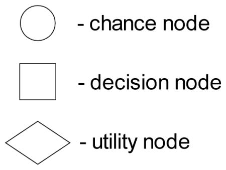
An influence diagram contains three kinds of nodes: chance (or uncertainty) nodes representing random variables; decision nodes representing decisions to be made; and one utility node, which is a random variable whose possible values are the utilities of the outcomes. We depict these nodes as follows:

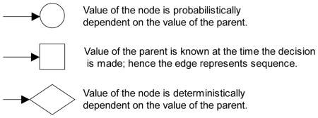
The edges in an influence diagram have the following meaning:

The chance nodes in an influence diagram constitute a Bayesian network. So an influence diagram is actually a Bayesian network augmented with decision nodes and a utility node. There must be an ordering of the decision nodes in an influence diagram based on the order in which the decisions are made. The order is specified using the edges between the decision nodes. An influence diagram is solved by determining the decision alternative of the first decision that maximizes expected utility. Specialized Bayesian network inference algorithms do this task [8].

The influence diagram in Figure 4 is the simplest such diagram since it has only one chance node. Next, we present a slightly more complex influence diagram. Suppose Sam has the opportunity to buy a 1996 Spiffycar automobile for $10,000, and he had a prospect that would be willing to pay $11,000 for the auto if it were in excellent mechanical shape. Suppose further that if the transmission is bad, Sam will have to spend $3000 to repair it before he could sell the vehicle. So he would only end up with only $8000 if he bought the vehicle and its transmission was bad. Finally, suppose Sam has a friend who could run a test on the transmission, and we have the following:

$$\begin{array}{l}P(\mathit{Test}=\mathit{positive}\mid \mathit{Tran}=\mathit{good})=0.3\\ P(\mathit{Test}=\mathit{positive}\mid \mathit{Tran}=\mathit{bad})=0.9\\ \hfill P(\mathit{Tran}=\mathit{good})=\mathrm{0.8.}\hfill \end{array}$$

Figure 5 shows an influence diagram representing this problem. Notice that there is an arrow from Tran to Test because the value of the test is probabilistically dependent on the state of the transmission, and there is an arrow from Test to D because the outcome of the test will be known at the time the decision is made. That is, D follows Test in sequence.

Figure 5.

An influence diagram representing the decision concerning buying the Spiffycar.

As mentioned previously, specialized Bayesian network inference algorithms are used to solve influence diagrams. In this case, if the test is positive the algorithm would determine that

$$EU(d1)=\$9714,$$

where EU denotes “expected utility”. On the other hand, if the test is negative the algorithm would determine that

$$EU(d1)=\$10,897.$$

Regardless of the test outcome, we have that

$$EU(d2)=\$10,000.$$

So the decision would be to buy the car if the test came back negative, and not to buy it if the test came back positive.

When the probabilities in an influence diagram are obtained from data, they are only estimates of assumed objective relative frequencies. So, our recommended decision might not be the one obtained using these relative frequencies. Neapolitan [16] develops a method for computing the probability that the recommended decision is the one which would be obtained using the objective relative frequencies. This probability is called the confidence in the decision.

We have only touched on decision analysis and influence diagrams. For a more thorough introduction see [17].

Quality Adjusted Life Expectancy

In medical applications, the utility is often life expectancy. However, living in disease states and living with treatments that have unpleasant side effects are not the same as living in perfect health. So, we adjust for quality of life when comparing sick years and treatment years to well years. As an example, suppose Andrea is considering a kidney transplant. One option for her is simply to stay on dialysis. However, living on dialysis is not equivalent to living in perfect health. So we ask Andrea to determine what one year of life on dialysis is worth relative to one well year of life. Let's say she says it is worth 0.6 “well” years. Then for Andrea

$$1\text{year}\text{on}\text{dialysis}\text{is}\text{equivalet}\text{to}0.6\text{well}\text{years}.$$

The value 0.6 is called the time-trade-off quality adjustment or quality-adjusted life year for dialysis. Another way to look at it is that Andrea would give up 0.4 years of life to avoid being on dialysis for 0.6 years. Note that the quality-adjusted life year is patient specific. Another individual might feel that 1 year on dialysis is equivalent to 0.5 well years. When we compute life expectancy using time-trade-off quality adjustment, we call it quality adjusted life expectancy (QALE).

Kidney Transplant Decision

A recently developed decision support tool for the kidney transplant decision is the Kidney Donor Risk Index. We briefly describe that index and problems with it, and then show how an influence diagram decision support tool could resolve those problems.

Kidney Donor Risk Index

The study that developed the Kidney Donor Risk Index (KDRI) analyzed 69,440 kidney transplant recipients, who received deceased donor transplants [7]. The study determined the following 14 independent donor and transplant factor predictor variables: donor age, race, hypertension, diabetes, serum creatinine, cerebrovascular cause of death, height, weight, donation after cardiac death, hepatitis C virus status, human leukocyte antigen-B and DR mismatch, cold ischemia time, en bloc transplant, and double transplant. The outcome variable was graft failure, defined as return to dialysis, retransplant, or death. Cox regression was used to model survival prediction. For a given transplant decision, the KDRI produces a risk index for the rate of graft failure relative to that of a healthy 40-year old donor. The risk index for a healthy 40 year old donor is set to 1. If the KDRI is, for example, 1.28 then the estimated increase in graft failure risk is 28%.

There are a several difficulties with the KDRI:

1. Cox regression analysis was used to predict survival. However, several difficulties have been noted with the model. First, its proportional hazards assumption is not necessarily justified in all cases [18,19]. Second, the purpose of a Cox model is more to identify covariates than to predict survival. Both a Bayesian network method [20] and a random forest method [21] have been shown to outperform the Cox model at survival prediction.

2. The KDRI does not model the interactions among variables to affect survival outcome. The biomedical community has shown an increased interest in modeling interactions, motivated partly by the efforts to learn how genes interact epistatically to affect disease [22]. However, interactions can be occurring amongst any set of variables. In particular, Zeng et al. [23] showed that tumor histology interacts with menopausal status to affect breast cancer death survival, but neither variables is correlated with survival by itself. Certainly, variables can also be interacting to affect graft failure. For example, height and weight might interact. That is, the risk for a 5′ 6″ 200 lb donor might be greater than the risk for a 6′ 2′ 200 lb donor.

3. The KDRI does not model recipient variables such as age, height, etc. However, these variables might also interact with donor variables.

4. The KDRI only informs us of relative risk. It does not tell the patient what can be expected if the kidney is accepted. In particular, it does not provide a measure of the expected quality of life if the kidney is accepted versus the expected quality of life if the patient stays on dialysis.

An Influence Diagram for the Kidney Transplant Decision

All four problems just identified can be resolved by developing an influence diagram using a dataset such as the one used in the KDRI study. However, this would be a major research project. Next we just illustrate a schema for such an influence diagram by considering only one variable, namely whether the patient has high Panel Reactive Antibody, which measures the antihuman antibodies in the blood. For the purpose of the example we do not take into consideration that for living donors, Donor Specific Antibodies are used today to determine appropriateness of matching.

We model the decision of whether to accept an incompatible kidney offered by a live donor or to wait for a compatible kidney to become available. The incompatible kidney has a higher risk of failing. A high Panel Reactive Antibody (PRA) is known to increase this risk of graft failure. If a kidney transplant has good graft function, both the likelihood of survival and the quality of life are better than if the patient stays on dialysis. On the other hand, if the kidney fails, both likelihood of survival and quality of life might be better when staying on dialysis.

We provide a simple model of this problem in which we assume a kidney transplant only occurs at time now (year 0), exactly one year later (end of year 1), exactly two years later (end of year 2), and so on. We also only have a three year time horizon. In application, the time discretization could be more refined, and the time horizon could be longer. Furthermore, we only model that the patient can make the decision once at time now. With some probability the opportunity for the live donor transplant will be available in the future, and these future decisions can also be modeled. Figure 6 shows an influence diagram representing this problem using the Bayesian network package Netica [24]. The Netica diagram shows the prior probability of the chance nodes rather than conditional probability distributions, and also the expected values of the utilities of the alternatives for the first decision.

Figure 6.

An influence diagram modeling the decision whether to accept a live donor kidney.

The decision node, which appears on the far left, represents the decision whether to “take live donor” or “wait”. The node “donor_kidney_year0” is a deterministic node which has the value “yes” if the decision was to take the live donor and the value “no” otherwise. That node affects the node “transplant0_works”, which represents whether the transplanted kidney works. Its value is “null” if the value of its parent is “no”. That node affects the node “dieyear1” which represents whether the patient dies in the first year, the node “dieyear2” which represents whether the patient dies in the second year, and the node “dieyear3” which represents whether the patient dies in the third year. The node “waitlist_kidney_year1” represents whether the patient receives a kidney in the first year if the decision was to wait. That node affects “transplant1_works” which represents whether the waitlist kidney obtained the first year takes. The node “waitlist_kidney_year2” represents whether the patient receives a kidney in the second year if the decision was to wait.

The utility nodes are on the far right. There is one node for each year. Each node’s value is 1 (year) if the patient lived the year in perfect health, and the value is a quality adjusted life year if the patient lived the year in less than perfect health. We assigned the quality adjustments based on feasible approximations; not on studies. They are not meant to be used in an actual system. The table for the first utility nodes follows.

U1	dieyear1	transplant0_takes
0	die	yes
0	die	no
0	die	null
1	live	yes
0.25	live	no
0.5	live	null

Let’s look at the utilities in the preceding table. If the patient dies, the utility is 0. On the other extreme, if the person has the transplant, it works, and the person lives, the utility is 1. If the person has the transplant and it does not work, the quality-adjusted life year has value 0.25. If the person does not have the transplant and stays on dialysis, the quality-adjusted life year has value 0.5. The table for the second utility node follows. The third utility node has similar values. However, we do not show its table because it has 4 parents, and so the table is very large.

U2	dieyear2	transplant1_takes	transplant0_takes
0	die	yes	yes
0	die	yes	no
0	die	yes	null
0	die	no	yes
0	die	no	no
0	die	no	null
0	die	null	yes
0	die	null	no
0	die	null	null
1	live	yes	yes
1	live	yes	no
1	live	yes	null
0.25	live	no	yes
0.25	live	no	no
0.25	live	no	null
1	live	null	yes
0.25	live	null	no
0.5	live	null	null

The expected utilities of the decision alternatives appear in the decision node. In this case, the expected utility is the QALE. Looking at the decision node, we see that the QALE (based on a 3 year time horizon) of decision “take live donor” is 2.4949 and the QALE of “wait” is 1.86275. So, the decision would be to take the donor kidney if we did not know the PRA value. Figure 7 shows the influence diagram with PRA instantiated to high. Now the recommended decision is to wait.

Figure 7.

The influence diagram in Figure 6 with PRA instantiated to high.

We only modeled one predictor variable (PRA) that affects the outcome variables. With a good dataset such as the one used in the KDRI study, we have hope to develop a system that models all relevant predictors, and is capable of providing personalized transplant decisions.

Glossary

Bayesian network

A graphic model that succinctly represents a joint probability distribution. It consists of a directed acyclic graph (DAG) in which each node represents a random variable, and the conditional probability distribution of each node given its parents in the DAG.

clinical decision support system (CDSS)

A computer program, which is designed to assist healthcare professionals with decision making tasks, such as determining the diagnosis and treatment of a patient.

decision analysis

The discipline that formally analyzes decision alternatives, and recommends the alternative that maximizes the expected utility of the outcome to the decision maker.

decision tree

A tree-like graph that models decision alternatives, their possible outcomes, and the utilities of the outcomes. It is used to recommend the decision alternative that maximizes expected utility.

influence diagram

A Bayesian network augmented with decision nodes and value nodes. It models the same problems as a decision tree, and is used to recommend the decision alternative that maximizes expected utility.

kidney donor risk index (KDRI)

A risk index for rate of graft failure relative to that of a healthy 40-year old donor.

quality adjusted life expectancy (QALE)

Life expectancy computed using a time-trade-off quality of life adjustment.

References

- 1.http://www.nih.gov/precisionmedicine/.
- 2.Schleinitz MD, DePalo D, Blume J, Stein M. Can differences in breast cancer utilities explain disparities in breast cancer care? J Gen Intern Med. 2006;21(12):1253–1260. doi: 10.1111/j.1525-1497.2006.00609.x. [DOI] [PMC free article] [PubMed] [Google Scholar]
- 3.Brennan VK, Wolowacz SE. A systematic review of breast cancer utility weights. Presented at ISPOR 13th Annual International Meeting; May 2008. [Google Scholar]
- 4.Peasgood T, Ward SE, Brazier J. Health-state utility values in breast cancer. Expert Rev Pharmacoecon Outcomes Res. 2010;10(5):553–566. doi: 10.1586/erp.10.65. [DOI] [PubMed] [Google Scholar]
- 5.Musen MA, Shahar Y, Shortliffe EH. Clinical Decision-Support System. In: Shortliffe EH, Cimino J, editors. Computer Applications in Health Care and Biomedicine. NY, NY: Springer; 2006. [Google Scholar]
- 6.Wyatt J, Altman D. Commentary: prognostic models: Clinically useful or quickly forgotten. British Medical Journal. 1995;311:1539–1541. [Google Scholar]
- 7.Rao PS, Schaubel DE, Guidinger MK. A comprehensive risk quantification score for deceased donor kidneys: the kidney donor risk index. Transplantation. 2009;88(2):231–236. doi: 10.1097/TP.0b013e3181ac620b. [DOI] [PubMed] [Google Scholar]
- 8.Neapolitan RE. Probabilistic Reasoning in Expert Systems. NY, NY: Wiley; 1989. [Google Scholar]
- 9.Neapolitan RE. Learning Bayesian Networks. Upper Saddle River, NJ: Prentice Hall; 2004. [Google Scholar]
- 10.Korb K, Nicholson AE. Bayesian Artificial Intelligence. Boca Raton, FL: Chapman & Hall/CRC; 2003. [Google Scholar]
- 11.Pearl J. Probabilistic Reasoning in Intelligent Systems. Burlington, MA: Morgan Kaufmann; 1988. [Google Scholar]
- 12.Segal E, Pe'er D, Regev A, Koller D, Friedman N. Learning module networks. Journal of Machine Learning Research. 2005;6:557–588. [Google Scholar]
- 13.Friedman N, Linial M, Nachman I, Pe'er D. Using Bayesian networks to analyze expression data. Proceedings of the Fourth Annual International Conference on Computational Molecular Biology; 2005; [DOI] [PubMed] [Google Scholar]
- 14.Fishelson M, Geiger D. Optimizing exact genetic linkage computation. Journal of Computational Biology. 2004;11(2–3):263–275. doi: 10.1089/1066527041410409. [DOI] [PubMed] [Google Scholar]
- 15.Neapolitan RE. Probabilistic Reasoning in Bioinformatics. Burlington, MA: Morgan Kaufmann; 2009. [Google Scholar]
- 16.Neapolitan RE. Computing the confidence in a medical decision obtained from an influence diagram. Artificial Intelligence in Medicine. 1993;5(4):341–363. doi: 10.1016/0933-3657(93)90021-t. [DOI] [PubMed] [Google Scholar]
- 17.Neapolitan RE, Jiang X. Probabilistic Methods for Financial and Marketing Informatics. Burlington, MA: Morgan Kaufmann; 2007. [Google Scholar]
- 18.Therneau TM, Grambsch PM. Modeling Survival Data: Extending the Cox Model. New York, NY: Springer; 2000. [Google Scholar]
- 19.Aalen OO. A linear regression model for the analysis of life times. Stat Med. 1989;8:907–925. doi: 10.1002/sim.4780080803. [DOI] [PubMed] [Google Scholar]
- 20.Jiang X, Xue D, Brufsky A, et al. A new method for predicting patient survivorship using efficient Bayesian network learning. Cancer Informatics. 2014;13:47–57. doi: 10.4137/CIN.S13053. [DOI] [PMC free article] [PubMed] [Google Scholar]
- 21.Lowsky DJ, Ding Y, Lee DKK, et al. A k-nearest neighbors survival probability prediction system. Stat Med. 2012;32(12):2062–9. doi: 10.1002/sim.5673. [DOI] [PubMed] [Google Scholar]
- 22.Hahn LW, Ritchie MD, Moore JH. Multifactor dimensionality reduction software for detecting gene-gene and gene-environment interactions. Bioinformatics. 2003;19:376–382. doi: 10.1093/bioinformatics/btf869. [DOI] [PubMed] [Google Scholar]
- 23.Zeng Z, Jiang X, Neapolitan R. Exhaustively searching for interactions using Bayesian network scoring and information gain. doi: 10.1186/s12859-016-1084-8. Submitted to BMC Bioinformatics 2016. [DOI] [PMC free article] [PubMed] [Google Scholar]
- 24.https://www.norsys.com/index.html.