Within-subject Pooling of Biological Samples to Reduce Exposure Misclassification in Biomarker-based Studies

Supplemental Digital Content is available in the text.

Background:

For chemicals with high within-subject temporal variability, assessing exposure biomarkers in a spot biospecimen poorly estimates average levels over long periods. The objective is to characterize the ability of within-subject pooling of biospecimens to reduce bias due to exposure misclassification when within-subject variability in biomarker concentrations is high.

Methods:

We considered chemicals with intraclass correlation coefficients of 0.6 and 0.2. In a simulation study, we hypothesized that the chemical urinary concentrations averaged over a given time period were associated with a health outcome and estimated the bias of studies assessing exposure that collected 1 to 50 random biospecimens per subject. We assumed a classical type error. We studied associations using a within-subject pooling approach and two measurement error models (simulation extrapolation and regression calibration), the latter requiring the assay of more than one biospecimen per subject.

Results:

For both continuous and binary outcomes, using one sample led to attenuation bias of 40% and 80% for compounds with intraclass correlation coefficients of 0.6 and 0.2, respectively. For a compound with an intraclass correlation coefficient of 0.6, the numbers of biospecimens required to limit bias to less than 10% were 6, 2, and 2 biospecimens with the pooling, simulation extrapolation, and regression calibration methods (these values were, respectively, 35, 8, and 2 for a compound with an intraclass correlation coefficient of 0.2). Compared with pooling, these methods did not improve power.

Conclusion:

Within-subject pooling limits attenuation bias without increasing assay costs. Simulation extrapolation and regression calibration further limit bias, compared with the pooling approach, but increase assay costs.

Exposure assessment is a central issue in epidemiologic studies exploring the effects of environmental contaminants on human health. For chemicals with multiple exposure sources, biomarker measurements in biospecimens are often used to assess an exposure proxy.^1,2 Such biomarker-based studies generally rely on few (often only one) biospecimens per subject. However, for chemicals with a short half-life, such as bisphenol A, phthalates, and pyrethroid pesticides, within-subject biomarker concentrations strongly vary over time.^3–5 Consequently, a biomarker assay based on a single biospecimen is likely to imperfectly reflect the average exposure throughout long time periods (typically, a week to several years). In this setting, the biomarker concentration measured in a spot biospecimen varies around the true unmeasured value (corresponding to the average biomarker level during the toxicologically relevant exposure window) in a way such that the average of many replicate measurements is expected to approximate the true individual level. This corresponds to what is termed classical error.⁶ Classical error is expected to bias dose–response relationships toward the null in a predictable way^7,8 and reduce statistical power.^9–11

Performing repeated exposure measurements on each study participant is generally a relevant option to reduce bias due to exposure misclassification in environmental health studies.^7,8 This approach has so far little been used in epidemiologic studies on the health effect of chemicals with short half-lives.^12,13 This might be due to the increased assay costs, and possibly to the assumption that increasing the number of study subjects is more efficient than increasing the number of biospecimens per subject (which is not always true¹⁴). One way to have some of the benefits of the reliance on repeated biospecimens per subject without increasing the assay costs, compared with the situation where only one biospecimen is collected, would be to collect and pool several biospecimens for each subject before assaying the chemical of interest (within-subject pooling). Pooling biospecimens from different subjects (between-subject pooling) has been applied since the 1940s to reduce the cost of identification of infectious cases in large populations.^15,16 More recently, in the context of case–control studies with expensive biomarker assays, between-subject pooling of biospecimens from random groups of cases and controls has been used to estimate individual effect of exposure while reducing assay costs.¹⁷ To the best of our knowledge, in spite of its simplicity, within-subject pooling of biospecimens has been very little used in biomarker-based environmental epidemiology. Notably, within-subject pooling has been proposed to limit the proportion of biospecimens with biomarker concentrations below the limit of detection,¹⁸ and as a strategy to estimate intraclass correlation coefficients (ICC).¹⁶

Our aim was therefore to assess the ability of within-subject pooling of biospecimens to reduce bias due to exposure misclassification occurring when biomarkers with strong temporal variability are considered. We compared the performance of this pooling approach to measurement error models, as approaches supposed to make optimal use of the collection of repeated biospecimens to adjust for measurement error.

METHODS

Overview of the Approach

We supposed that one is interested in estimating the health effects of exposure during a specific time-window to two distinct nonpersistent chemicals with different temporal variability in a biological matrix such as urine. We used different approaches to study the associations between the biomarker concentrations assayed with error in repeated biospecimens in each subject and continuous (e.g., child weight at the age of 3 years) and binary (e.g., being overweight) health outcomes: within-subject pooling of biospecimens before assaying the chemical (or pooling method, possibly followed by a posteriori disattenuation^7,8) and two measurement error models relying on the assay of the chemical in each biospecimen: regression calibration and simulation extrapolation (SIMEX). We simulated epidemiologic studies conducted in the general population and estimated bias and statistical power for the four approaches.

Simulation of Exposures

For each subject i (i = 1, …, n) a variable X_i, drawn at random from a normal distribution (mean, 0; standard deviation (SD) σ_X = 1), was assumed to represent the real unobserved average concentration (in μg/liter) of the considered chemical in the biospecimens collected over a toxicologically relevant exposure window, measured without error, after standardization and centering around 0.

For each subject, we generated 50 error-prone variables W_ij (j = 1, …, 50) corresponding to exposure biomarker concentrations assayed in spot biospecimens collected at random time points during the relevant exposure window. W_ij is an error-prone estimate of X_i. The within-subject error (U_{ij, within}, mean 0; SD, ) affecting W_ij was supposed to be related to the individual and might be due to the variability in urinary concentrations arising from the toxicokinetics of the studied compound, temporal variations in diluteness of the urine and temporal variability in exposure itself. U_{ij, within} was assumed to correspond to random variations around the real value X_i, to be additive and of classical type. The variance of the error term U_{ij, within} was computed as¹⁹

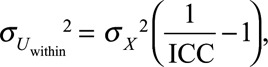(1)

where ICC is the intraclass correlation coefficient, corresponding to the expected correlation between biomarker concentrations in any pair of biospecimens W_ij and W_ik collected at different time points during the exposure window of interest. ICCs were set at 0.6 (moderate within-subject variability, chemical A) or 0.2 (high within-subject variability, chemical B). ICCs of about 0.6 have been typically reported for benzophenone-3, parabens, and a butylbenzylphthalate metabolite, while ICCs of 0.1–0.2 have been reported for bisphenol A and di-(2-ethylhexyl) phthalate (DEHP) metabolites.^20,21

In additional analyses, we also considered between-assay error (U_{ij, assay}) due to the biomarker measurement and arising from the technician and from analytical error (see eTables 1, 2; http://links.lww.com/EDE/B27).

In most simulations, we assumed the number of biospecimens to be the same for each subject (balanced design). We additionally specifically considered the situation of an unbalanced number of biospecimens per subject keeping constant the total number of subjects (n = 3,000) as well as the total number of biospecimens available in the population (n = 9,000).

Simulation of Health Outcomes

We simulated the continuous outcome Y_i as

(2)

where β₁, the “real” effect of the chemical on Y, was assumed to be −100 g for each increase by 1 in X and ε was a normally distributed random error (mean = 0). The values of α (14,900 g) and of the standard deviation of ε (1,650 g) were based on the values observed for the weight at 3 years in a mother-child cohort (Eden cohort,²²). To study the impact of measurement error on the risk of type 1 error, we also conducted simulations assuming a lack of effect of exposure (β₁ = 0).

We also simulated the case of a binary heath outcome (see eTables 3, 4; http://links.lww.com/EDE/B27).

Characterizing Bias in Studies Relying on Error-prone Estimates of Exposure

Within-subject Pooling

This method consisted of regressing the outcome Y over an exposure variable corresponding to the biomarker concentration measured in the pool of k (k = 1, …, 50) random (error-prone) biospecimens from each subject. We assumed that all individual specimens were pooled in equal volume, and errors that could arise from pooling volumes of individual specimens that were not exactly equal were not considered. Associations between the concentration measured in the pool (average of W_i1…W_ik) and each health outcome were characterized by linear and logistic regression models for the continuous and binary health outcomes, respectively.

In the situations of unbalanced numbers of biospecimens pooled per participant, we used weighted linear and logistic regression models to assess associations between exposure and outcome. We used analytical weights depending on the number of biospecimens available for each participant; these weights were inversely proportional to the variance of the subject-specific exposure average (option aweight in Stata).

A Posteriori Disattenuation

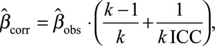
In the balanced design, we additionally corrected the effect estimates from the pooling method^7,8:

(3)

where was the observed effect estimate with the pooling method, ICC the intraclass correlation coefficient, and K the number of biospecimens pooled per subject. The same correction was applied to the standard deviation.

Measurement Error Models

We considered two measurement error models (SIMEX and regression calibration^11,23), which make use of the assay of several biospecimens per subject to correct the dose–response function. For SIMEX, we used a quadratic model for the extrapolation step. We used bootstrap with 100 replications to estimate the variance of the estimated effects for both models. The models were implemented in Stata using the commands rcal for regression calibration²⁴ and simex for simulation extrapolation²⁵ (http://www.stata.com/merror; see eAppendix 1 for more details; http://links.lww.com/EDE/B27).

For each of the two chemicals considered, 1,000 studies were simulated. For each method, we quantified the average effect estimate () and the statistical power, defined as the proportion of studies in which the P value of the parameter characterizing the association between the error-prone variables and the health outcome was below 0.05. Results are presented for a sample size of 3,000 subjects and with the default assumption of lack of between-assay error, unless otherwise specified.

Simulations and analyses were performed using STATA/SE, version 13 (StataCorp, College Station, TX). Our code for the continuous outcome is provided in the Supplemental Material (eAppendix 2, the code for the binary outcome is available upon request; http://links.lww.com/EDE/B27).

RESULTS

Distributions of X, W, and U_ij,within and the simulated concentrations for three subjects are shown in eFigures 1 and 2 (http://links.lww.com/EDE/B27).

Bias Resulting from the Use of One Urine Sample to Assess Exposure

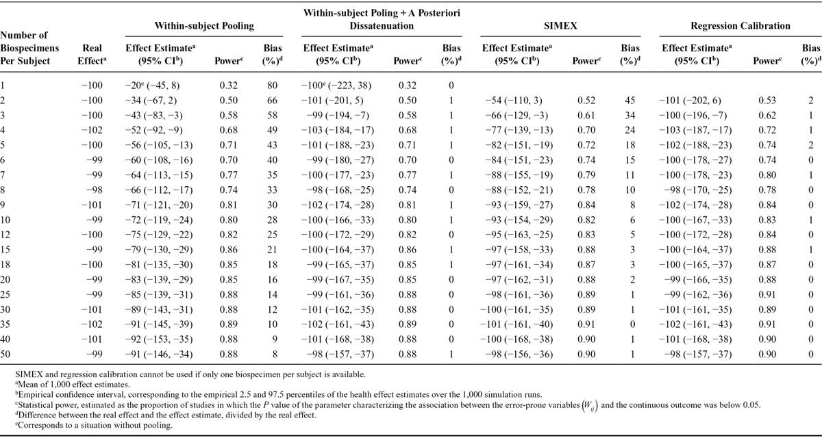
For chemical A (ICC of 0.6), the reliance on one urine sample to assess exposure led to an estimated effect of −60 g (average over 1,000 studies), corresponding to an attenuation by 40% compared with the real effect (β₁ = −100 g). Statistical power was 71% with a sample size of 3,000 subjects (Table 1). For chemical B (ICC of 0.2), when using one sample, the average effect estimate was −20 g (attenuation bias of 80%) and power was 32% (Table 2). Bias in the logarithm of the estimated odds-ratio associated with the exposure variable and power were similar for the binary outcome (eTables 3, 4; http://links.lww.com/EDE/B27).

TABLE 1.

Effect Estimates and Statistical Power of Studies Aiming at Characterizing the Association Between Biomarker-based Exposure to Chemical A (Intraclass Correlation Coefficient, 0.6) and a Continuous Health Outcome, According to the Number of Biospecimens Collected Per Subject and the Approach Used to Limit the Effect of Exposure Misclassification (1,000 Simulations of Studies with 3,000 Subjects Each; Real Effect β1 = −100 g, Assuming Lack of Between-assay Error)

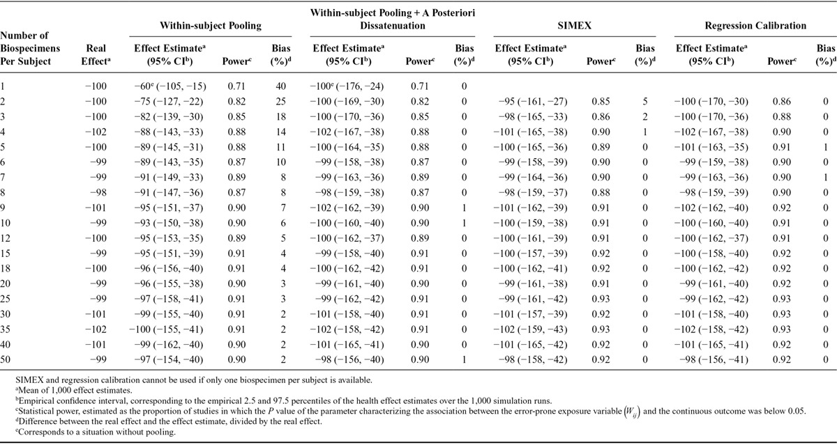
TABLE 2.

Effect Estimates and Statistical Power of the Simulated Studies Aiming at Characterizing the Association Between Biomarker-based Exposure to Chemical B (Intraclass Correlation Coefficient, 0.2) and a Continuous Health Outcome, According to the Number of Biospecimens Collected Per Subject and the Approach Used to Limit Exposure Misclassification (1,000 Simulations of Studies with 3,000 Subjects Each; Real Effect β1 = −100 g, Assuming Lack of Between-assay Error)

For the continuous outcome, dividing the observed effect estimates by the ICC (a posteriori disattenuation^7,8) yielded corrected effect estimates of −100 g on average (i.e., no bias) for both chemicals. A posteriori disattenuation did not improve power (Tables 1, 2).

Increasing the Number of Biospecimens

Using the concentration assayed in the pool of several biospecimens per subject as a proxy of exposure decreased bias (Figure) and increased power, compared with the situation where one biospecimen was used per participant and no a posteriori disattenuation was applied. For both the continuous (Tables 1, 2) and binary (eTables 3, 4; http://links.lww.com/EDE/B27) outcomes, the number of biospecimens per subject required to limit the bias in the health effect estimate to 10% was 6 for chemical A (ICC of 0.6, Table 1, eTable 3; http://links.lww.com/EDE/B27) and 35 for chemical B (ICC of 0.2, Table 2, eTable 4; http://links.lww.com/EDE/B27). These values were reduced to 1 biospecimen when a posteriori disattenuation correction was applied.

FIGURE.

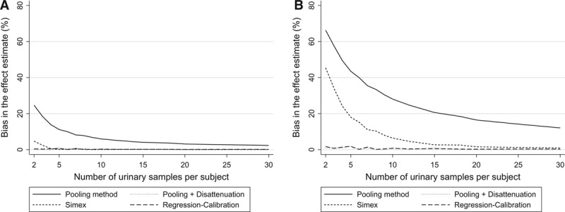
Bias in the health effect estimate (%) according to the number of biospecimens collected per subject to assess exposure (1,000 simulations of studies with 3,000 subjects each; continuous health outcome, real effect β₁ = −100 g, (assuming lack of between-assay error, = 0). A, Compound A (ICC of 0.6). B, Compound B (ICC of 0.2).

Applying Measurement Error Models

For a given number of biospecimens, SIMEX and regression calibration drastically reduced bias compared with pooling without disattenuation (Figure). As an example, for an ICC of 0.6 and considering a continuous health outcome, using two biospecimens per subject led to effect estimates biased by 25%, 5%, and 0% with pooling, SIMEX, and regression calibration, respectively (Table 1); these values were respectively 66%, 45%, and 2% for a compound with an ICC of 0.2 (Table 2). Statistical power was similar (slightly higher) for SIMEX, regression calibration, and the pooling approach: for chemical B (ICC of 0.2) and considering a continuous health outcome, collecting two biospecimens led to a power of 50% for the pooling method, 52% for SIMEX, and 53% for regression calibration (study sample size of 3,000, Table 2).

Impact of Exposure Misclassification on Type 1 Error

When the real effect of exposure was assumed to be null and one biospecimen was used to assess exposure, the P value of the parameter associated with exposure was below 0.05 for 5% of the simulated datasets, whatever the ICC considered (eTables 5, 6; http://links.lww.com/EDE/B27), suggesting that under the hypotheses of our simulations, using one biospecimen to assess exposure did not increase the risk of type 1 error. For a given number of biospecimens, the risk of type I error was slightly higher with SIMEX and regression calibration (range: 5%–8%) compared with the pooling approach (range: 4%–6%, eTables 5, 6; http://links.lww.com/EDE/B27).

Unbalanced Number of Biospecimens Between Subjects

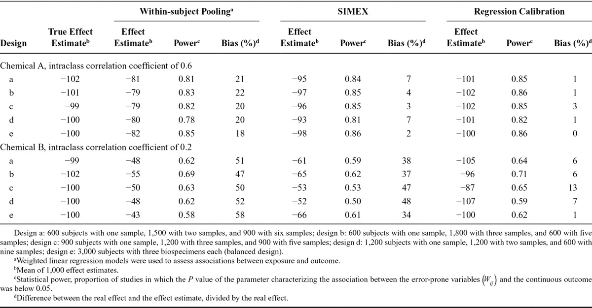
For chemical A (ICC of 0.6), and for a given total number of biospecimens collected (9,000 samples among 3,000 subjects), bias in the effect estimate was slightly higher when the design was unbalanced (different numbers of biospecimens per subject, bias 20%–22%) than when the design was balanced (bias of 18%, Table 3). For chemical B (ICC of 0.2), the effect estimate tended to be less biased with unbalanced (47%–52%) compared with balanced (58%) designs (Table 3). When measurement error models were applied, bias was always lower with a balanced design than with unbalanced designs (Table 3).

TABLE 3.

Unbalanced Designs: Effect Estimates and Statistical Power When the Numbers of Biospecimens Available Differed Between Subjects (Continuous Outcome, 1,000 Simulations for Each Design; Real Effect β1 = −100, Assuming a Lack of Between-assay Error)

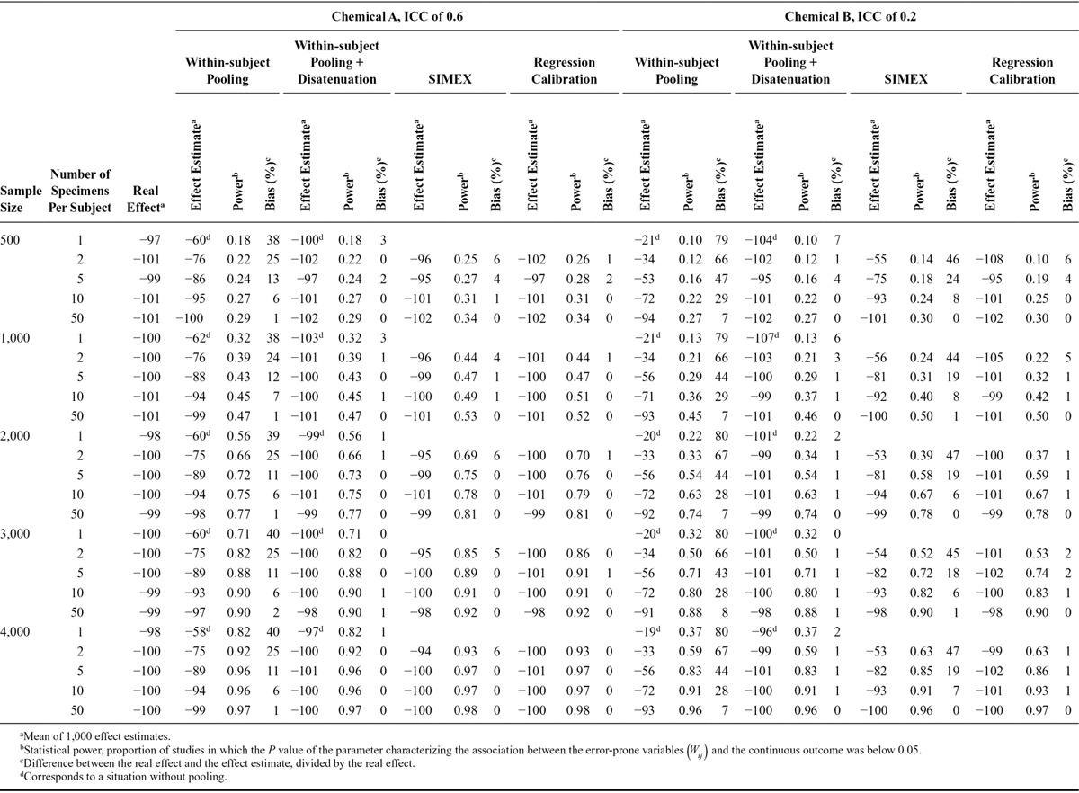
Impact of Study Sample Size

Overall, for a given number of biospecimens per participant, varying study sample size did not affect bias but impacted statistical power (Table 4). For both ICCs, we observed higher bias and higher statistical power in studies relying on one biospecimen per subject compared with studies with two pooled biospecimens and half the sample size (Table 4). For compounds with an ICC of 0.2, the loss of power when recruiting half as many subjects with twice as many biospecimens was sometimes limited: power was 37% for a study of 4,000 subjects with one biospecimen per subject, and 33% in a study of 2,000 subjects in which two biospecimens were pooled by subject; bias was lower (67%) in the latter study with 2,000 subjects than in the former one with 4,000 subjects (80%, Table 4).

TABLE 4.

Effect Estimates and Statistical Power of the Simulated Studies Aiming at Characterizing the Association Between a Biomarker-based Exposure and a Continuous Health Outcome According to the Number of Biospecimens Collected Per Subject, the Population Size and the Method Used to Study the Associations (1,000 Simulations for Each Population Size; Real Effect β1 = −100 g, Assuming a Lack of Between-assay Error)

Impact of Between-assay Error

For a given number of biospecimens, with the pooling method, bias increased with increasing between-assay error (eTable 1; http://links.lww.com/EDE/B27). When several biospecimens were available per subject, performance of a posteriori disattenuation was reduced with increasing between-assay error. For a compound with an ICC of 0.6, when five biospecimens were available per subject, a posteriori disattenuation led to effect estimates biased by 1%, 8%, and 31% for between-assay variances of 0.01, 0.1, and 0.5, respectively. With regression calibration, the between-assay variance did not affect bias while with SIMEX, bias increased with increasing between-assay error (eTable 1; http://links.lww.com/EDE/B27). This increase in bias is likely to result from the effect of the ICC decrease (from 0.60 to 0.46 and from 0.20 to 0.18) that resulted from the increase in the between-assay error, rather than result from a direct effect of the between assay error. Indeed, in simulations in which ICCs were kept constant whatever the value of the between-assay error, with SIMEX, bias was not affected by increases in the between-assay variance (eTable 2; http://links.lww.com/EDE/B27).

In situations of substantial between-assay error (, 0.1 and 0.5), power was lower with pooling compared with SIMEX and regression calibration (eTables 1, 2; http://links.lww.com/EDE/B27).

DISCUSSION

Our simulation study confirmed that relying on one biospecimen to assess exposure to short half-life chemicals yields biased dose–response functions. Increasing the number of biospecimens per subject and pooling them was efficient in decreasing bias and increasing statistical power without affecting assay costs, compared with the usual approach in which only one biospecimen per subject is collected. When the number of biospecimens pooled is identical for each subject, bias due to classical-type error could be further reduced by applying an a posteriori correction (disattenuation) to the effect estimate obtained with the pooling method.^7,8

Bias and Power in Studies Relying on One Biospecimen

The attenuation in the effect estimates observed in our study has been previously described in situations of measurement error of classical type.^7,8,10,11 When one biospecimen per subject was used to assess exposure, our results were in line with the property that the ICC corresponds to the multiplicative attenuation factor in the parameter of the regression model.^7,8 Consequently, if the ICC is known, dividing the observed effect estimate by the ICC (a posteriori disattenuation) provided unbiased estimate of the real effect. Such a correction did not improve power. For compounds with low ICCs, such as bisphenol A, DEHP metabolites and some pesticides (ICC below 0.3),^21,26,27 the bias in studies relying on a single biospecimen per subject appears very large (more than 70% attenuation), making such studies of limited informative value regarding the dose–response function whatever the number of subjects. Bias remains large with an ICC of 0.6.

The decrease in power observed with decreasing ICC was coherent with the fact that the bias in the health effect estimates corresponded to attenuation.¹¹ As discussed elsewhere,²⁸ when several chemicals with different ICCs are simultaneously considered,^29,30 interpretation of results should consider these ICCs, in particular when no association is highlighted. Without bias correction, such studies cannot easily be used to identify which exposure, among those tested, is most harmful, because the amplitude of the bias is likely to differ between exposures.

Increasing the Number of Biospecimens Per Subject

Collecting repeated biospecimens per subject is an efficient method to decrease bias. The number of biospecimens that has to be collected to restrict attenuation of the health effect estimate can be estimated from the formula from Brunekreef et al.,⁸ and Rappaport et al.⁷ (Eq. 3), which predicts that six and 36 biospecimens per participants would be needed to limit the attenuation factor to 0.9 for chemicals with ICCs of 0.6 and 0.2, respectively. This was in line with our estimations based on a simulation approach (six and more than 35 biospecimens, respectively). Most epidemiologic studies relying on biomarkers to assess exposure to short half-life compounds relied on a small number of biospecimens per subject.^13,22,31 A possible explanation lies in the increased cost incurred by the assessment of biomarkers in several biospecimens per subject. This is not a justification to refrain from collecting several biospecimens per subject. Indeed, the within-subject pooling approach described here allows to decrease bias and increase power without increasing assay costs, compared with the situation when one spot biospecimen is collected. When the number of biospecimens pooled is identical for each subject, a posteriori disattenuation^7,8 can be used to further reduce attenuation bias. If the number of samples collected varies between subjects (unbalanced design), then the formula to disattenuate effect estimates a posteriori cannot rigorously be used anymore, but, as we have illustrated, the within-subject pooling approach still applies.

When no a posteriori correction of the effect estimate was performed, for a given number of biospecimens collected, studies relying on one biospecimen were more biased but had higher power than studies with two pooled biospecimens and half the sample size. For a compound with an ICC of 0.2, the gain in power was sometimes limited. For such compounds, compared with studies with a single biospecimen, studies with two or more samples per subject and possibly fewer subjects are an alternative worth considering. These would moreover have a lower assay cost.

Limitations of the Within-subject Pooling Approach

For chemicals with high intraindividual variability (ICC of 0.2), without a posteriori disattenuation, a large number of biospecimens (above 30) was required for the pooling approach to limit bias to 10%. Collecting more than 30 samples per subject outside of a clinical setting is cumbersome for the subjects (possibly limiting participation rate and inducing selection bias) and in terms of collection, storage and processing of the biological samples, which might impact the total cost of the cohort.

Caution is required in attempting to correct biomarker levels for creatinine concentration when pooling is done. The mathematical average of the creatinine-standardized biomarker concentrations (biomarker concentration/creatinine concentration) assessed in two biospecimens will indeed generally differ from the creatinine-standardized concentration assessed in the pool made of these two biospecimens; this feature might limit the efficiency of creatinine correction through standardization in the pooling approach. Other approaches could be considered to take into account urine dilution.³²

If the toxicologically relevant exposure window is unknown, pooling biospecimens over long exposure windows should be considered with caution, as pooling biospecimens collected during the relevant exposure window with biospecimens collected in another exposure window may increase exposure misclassification instead of decreasing it, in particular if exposure varied between the two windows considered.

Use of Measurement Error Models to Decrease Bias

Compared with the pooling approach used without a posteriori disattenuation, for a given number of biospecimens per subject, SIMEX and regression calibration strongly reduced bias. In our simulations, for chemicals with moderate intraindividual variability (ICC of 0.6), both measurement error models behaved similarly and two biospecimens were enough to limit bias to 10%. For chemicals with high variability (ICC of 0.2), SIMEX appeared to be less able than regression calibration to reduce bias. In line with our results, studies relying on linear and logistic models overall observed more biased effect estimates with SIMEX than with regression calibration in the case of high intraindividual variability in exposure.^33,34

The slight gain in power observed with SIMEX and regression calibration compared with pooling is likely to result from the fact that, under the assumptions of our simulation, SIMEX and regression calibration led to inflated type I error, compared with pooling. The fact that, compared with pooling, measurement error models did not strongly improve power while reducing bias, is a manifestation of the bias versus variance tradeoff¹¹: measurement error models led to effect estimates that were less attenuated (further away from the null), but with larger variances than the effect estimates from the pooling approach.

SIMEX and regression calibration corrected for both the between-assay error and the error related to the individual, while the within-subject pooling method was inefficient in correcting for the between-assay error. An explanation is that, in contrast to the individual error, which tends to cancel out when several biospecimens are pooled, the between-assay error occurs after the pooling is done and remains the same whatever the number of biospecimens pooled. Conversely, SIMEX and regression calibration methods identified the total error (including the intraindividual and between-assay error) through the repeated assays and corrected for it.

Although measurement error models have been applied in air pollution^35,36 and nutritional^37,38 epidemiology, they have so far little been used in biomarker-based studies in the general population. Repeated measurements of exposure for each subject are needed to use these models; an option to limit the cost incurred by these repeated assessments is to perform them among a subsample of study subjects rather than the entire population.³⁸

Model Assumptions

Although no study actually tried to characterize the statistical nature (i.e., classical or Berkson-type errors) of the error entailed by within-subject biomarker variability, we believe that the assumption we made regarding the classical nature of error is plausible for biomarkers of exposure to widely used chemicals with short half-life in the general population. We assumed the correlation between two repeated measurements to be the same whatever the time elapsed between biospecimen collections, which might not be true for some short half-life compounds (correlation levels might for example decrease with time²¹). This might limit generalizability of our results. We assumed that all biomarker levels were above the limit of detection, which will generally not occur for all populations nor chemicals considered with the currently available bioassays. The proportion of samples with a concentration below the limit of detection will be lower in pooled than unpooled samples,^17,18 which may have caused us to overestimate the relative efficiency of measurement error models, compared with the pooling approach.

We assumed that the average of the concentrations measured in all biospecimens collected during the considered time window corresponded to the toxicologically relevant dose (or was a good proxy thereof). For some exposure–health outcome pairs, the toxicologically relevant measure of exposure may rather be the dose to a specific organ, of which the urinary concentration is only a proxy. These sources of exposure misclassification will possibly further bias dose–response relations in a way that we did not consider. Finally, we did not consider confounding and selection biases.

CONCLUSION

Biomarker-based studies dealing with compounds with an ICC of 0.6 or less can be strongly biased and weakly powered if only one biospecimen per subject is collected. Such studies should collect repeated biospecimens per subject. Assessing biomarker concentrations in each biospecimen allows, if measurement error models are used, to efficiently correct for both the between-assay error and the error related to the individual, but entails higher assay cost. The within-subject pooling approach that we described appears efficient in situations with low between-assay error and provides a less biased and more powerful design than if only one sample had been collected, without increasing assay costs. If the number of biospecimens pooled is identical for each participant, the pooling approach can be coupled with a posteriori bias disattenuation which, if a good estimate of the ICC is available for the studied chemical and under the assumption of a classical type error, further reduces bias.^7,8

ACKNOWLEDGMENTS

We acknowledge Irva Hertz-Picciotto for her support and Xavier Basagaña for a useful comment.

Supplementary Material

ede-27-378-s001.doc ^{(9.4MB, doc)}

REFERENCES

- 1.Calafat AM, Ye X, Silva MJ, Kuklenyik Z, Needham LL. Human exposure assessment to environmental chemicals using biomonitoring. Int J Androl. 2006;29:166–171; discussion 181. doi: 10.1111/j.1365-2605.2005.00570.x. [DOI] [PubMed] [Google Scholar]
- 2.Schisterman EF, Albert PS. The biomarker revolution. Stat Med. 2012;31:2513–2515. doi: 10.1002/sim.5499. [DOI] [PMC free article] [PubMed] [Google Scholar]
- 3.Ye X, Wong LY, Bishop AM, Calafat AM. Variability of urinary concentrations of bisphenol A in spot samples, first morning voids, and 24-hour collections. Environ Health Perspect. 2011;119:983–988. doi: 10.1289/ehp.1002701. [DOI] [PMC free article] [PubMed] [Google Scholar]
- 4.Preau JL, Jr, Wong LY, Silva MJ, Needham LL, Calafat AM. Variability over one week in the urinary concentrations of metabolites of diethyl phthalate and di(2-ethylhexyl) phthalate among 8 adults: an observational study. Environ Health Perspect. 2010;118:1748–1754. doi: 10.1289/ehp.1002231. [DOI] [PMC free article] [PubMed] [Google Scholar]
- 5.Wielgomas B. Variability of urinary excretion of pyrethroid metabolites in seven persons over seven consecutive days: implications for observational studies. Toxicol Lett. 2013;221:15–22. doi: 10.1016/j.toxlet.2013.05.009. [DOI] [PubMed] [Google Scholar]
- 6.Armstrong BG. Effect of measurement error on epidemiological studies of environmental and occupational exposures. Occup Environ Med. 1998;55:651–656. doi: 10.1136/oem.55.10.651. [DOI] [PMC free article] [PubMed] [Google Scholar]
- 7.Rappaport SM, Symanski E, Yager JW, Kupper LL. The relationship between environmental monitoring and biological markers in exposure assessment. Environ Health Perspect. 1995;103(Suppl 3):49–53. doi: 10.1289/ehp.95103s349. [DOI] [PMC free article] [PubMed] [Google Scholar]
- 8.Brunekreef B, Noy D, Clausing P. Variability of exposure measurements in environmental epidemiology. Am J Epidemiol. 1987;125:892–898. doi: 10.1093/oxfordjournals.aje.a114606. [DOI] [PubMed] [Google Scholar]
- 9.de Klerk NH, English DR, Armstrong BK. A review of the effects of random measurement error on relative risk estimates in epidemiological studies. Int J Epidemiol. 1989;18:705–712. doi: 10.1093/ije/18.3.705. [DOI] [PubMed] [Google Scholar]
- 10.Bateson TF, Wright JM. Regression calibration for classical exposure measurement error in environmental epidemiology studies using multiple local surrogate exposures. Am J Epidemiol. 2010;172:344–352. doi: 10.1093/aje/kwq123. [DOI] [PubMed] [Google Scholar]
- 11.Carroll RJ, Ruppert D, Stefanski LA. Measurement Error in Nonlinear Models: A Modern Perspective. 2nd ed. London: Chapman & Hall; 1995. [Google Scholar]
- 12.Braun JM, Kalkbrenner AE, Calafat AM, et al. Impact of early-life bisphenol A exposure on behavior and executive function in children. Pediatrics. 2011;128:873–882. doi: 10.1542/peds.2011-1335. [DOI] [PMC free article] [PubMed] [Google Scholar]
- 13.Snijder CA, Heederik D, Pierik FH, et al. Fetal growth and prenatal exposure to bisphenol A: the generation R study. Environ Health Perspect. 2013;121:393–398. doi: 10.1289/ehp.1205296. [DOI] [PMC free article] [PubMed] [Google Scholar]
- 14.Tielemans E, Heederik D, Burdorf A, Loomis D, Habbema DF. Intraindividual variability and redundancy of semen parameters. Epidemiology. 1997;8:99–103. doi: 10.1097/00001648-199701000-00016. [DOI] [PubMed] [Google Scholar]
- 15.Dorfman R. The detection of defective members of large populations. Ann Math Stat. 1943;14:436–440. [Google Scholar]
- 16.Malinovsky Y, Albert PS, Schisterman EF. Pooling designs for outcomes under a Gaussian random effects model. Biometrics. 2012;68:45–52. doi: 10.1111/j.1541-0420.2011.01673.x. [DOI] [PMC free article] [PubMed] [Google Scholar]
- 17.Weinberg CR, Umbach DM. Using pooled exposure assessment to improve efficiency in case-control studies. Biometrics. 1999;55:718–726. doi: 10.1111/j.0006-341x.1999.00718.x. [DOI] [PubMed] [Google Scholar]
- 18.Schisterman EF, Vexler A. To pool or not to pool, from whether to when: applications of pooling to biospecimens subject to a limit of detection. Paediatr Perinat Epidemiol. 2008;22:486–496. doi: 10.1111/j.1365-3016.2008.00956.x. [DOI] [PMC free article] [PubMed] [Google Scholar]
- 19.Veronesi G, Ferrario MM, Chambless LE. Comparing measurement error correction methods for rate-of-change exposure variables in survival analysis. Stat Methods Med Res. 2013;22:583–597. doi: 10.1177/0962280210395742. [DOI] [PubMed] [Google Scholar]
- 20.Adibi JJ, Whyatt RM, Williams PL, et al. Characterization of phthalate exposure among pregnant women assessed by repeat air and urine samples. Environ Health Perspect. 2008;116:467–473. doi: 10.1289/ehp.10749. [DOI] [PMC free article] [PubMed] [Google Scholar]
- 21.Philippat C, Wolff MS, Calafat AM, et al. Prenatal exposure to environmental phenols: concentrations in amniotic fluid and variability in urinary concentrations during pregnancy. Environ Health Perspect. 2013;121:1225–1231. doi: 10.1289/ehp.1206335. [DOI] [PMC free article] [PubMed] [Google Scholar]
- 22.Philippat C, Botton J, Calafat AM, Ye X, Charles MA, Slama R, EDEN Study Group EDEN Study Group. Prenatal exposure to phenols and growth in boys. Epidemiology. 2014;25:625–635. doi: 10.1097/EDE.0000000000000132. [DOI] [PMC free article] [PubMed] [Google Scholar]
- 23.Fuller WA. Measurement Error Model. New York, NY: John Wiley & Sons; 1987. [Google Scholar]
- 24.Hardin JW, Schmiediche H, Carroll RJ. The regression-calibration method for fitting generalized linear models with additive measurement error. Stata J. 2003;3:361–372. [Google Scholar]
- 25.Hardin JW, Schmiediche H, Carroll RJ. The simulation extrapolation method for fitting generalized linear models with additive measurement error. Stata J. 2003;3:373–385. [Google Scholar]
- 26.Braun JM, Kalkbrenner AE, Calafat AM, et al. Variability and predictors of urinary bisphenol A concentrations during pregnancy. Environ Health Perspect. 2011;119:131–137. doi: 10.1289/ehp.1002366. [DOI] [PMC free article] [PubMed] [Google Scholar]
- 27.Attfield KR, Hughes MD, Spengler JD, Lu C. Within- and between-child variation in repeated urinary pesticide metabolite measurements over a 1-year period. Environ Health Perspect. 2014;122:201–206. doi: 10.1289/ehp.1306737. [DOI] [PMC free article] [PubMed] [Google Scholar]
- 28.Slama R, Vrijheid M. Some challenges of studies aiming to relate the exposome to human health. Occup Environ Med. 2015;72:383–384. doi: 10.1136/oemed-2014-102546. [DOI] [PubMed] [Google Scholar]
- 29.Patel CJ, Yang T, Hu Z, et al. March of Dimes Prematurity Research Center at Stanford University School of Medicine. Investigation of maternal environmental exposures in association with self-reported preterm birth. Reprod Toxicol. 2014;45:1–7. doi: 10.1016/j.reprotox.2013.12.005. [DOI] [PMC free article] [PubMed] [Google Scholar]
- 30.Lenters V, Portengen L, Smit LA, et al. Phthalates, perfluoroalkyl acids, metals and organochlorines and reproductive function: a multipollutant assessment in Greenlandic, Polish and Ukrainian men. Occup Environ Med. 2015;72:385–393. doi: 10.1136/oemed-2014-102264. [DOI] [PubMed] [Google Scholar]
- 31.Braun JM, Kalkbrenner AE, Just AC, et al. Gestational exposure to endocrine-disrupting chemicals and reciprocal social, repetitive, and stereotypic behaviors in 4- and 5-year-old children: the HOME study. Environ Health Perspect. 2014;122:513–520. doi: 10.1289/ehp.1307261. [DOI] [PMC free article] [PubMed] [Google Scholar]
- 32.Christensen K, Sobus J, Phillips M, Blessinger T, Lorber M, Tan YM. Changes in epidemiologic associations with different exposure metrics: a case study of phthalate exposure associations with body mass index and waist circumference. Environ Int. 2014;73:66–76. doi: 10.1016/j.envint.2014.07.010. [DOI] [PubMed] [Google Scholar]
- 33.Batistatou E, McNamee R. Performance of bias-correction methods for exposure measurement error using repeated measurements with and without missing data. Stat Med. 2012;31:3467–3480. doi: 10.1002/sim.5422. [DOI] [PubMed] [Google Scholar]
- 34.Fung KY, Krewski D. Evaluation of regression calibration and SIMEX methods in logistic regression when one of the predictors is subject to additive measurement error. J Epidemiol Biostat. 1999;4:65–74. [PubMed] [Google Scholar]
- 35.Van Roosbroeck S, Li R, Hoek G, Lebret E, Brunekreef B, Spiegelman D. Traffic-related outdoor air pollution and respiratory symptoms in children: the impact of adjustment for exposure measurement error. Epidemiology. 2008;19:409–416. doi: 10.1097/EDE.0b013e3181673bab. [DOI] [PubMed] [Google Scholar]
- 36.Horick N, Weller E, Milton DK, Gold DR, Li R, Spiegelman D. Home endotoxin exposure and wheeze in infants: correction for bias due to exposure measurement error. Environ Health Perspect. 2006;114:135–140. doi: 10.1289/ehp.7981. [DOI] [PMC free article] [PubMed] [Google Scholar]
- 37.Beydoun MA, Kaufman JS, Ibrahim J, Satia JA, Heiss G. Measurement error adjustment in essential fatty acid intake from a food frequency questionnaire: alternative approaches and methods. BMC Med Res Methodol. 2007;7:41. doi: 10.1186/1471-2288-7-41. [DOI] [PMC free article] [PubMed] [Google Scholar]
- 38.Spiegelman D, McDermott A, Rosner B. Regression calibration method for correcting measurement-error bias in nutritional epidemiology. Am J Clin Nutr. 1997;65(4 Suppl):1179S–1186S. doi: 10.1093/ajcn/65.4.1179S. [DOI] [PubMed] [Google Scholar]