CHIMERA: Clustering of heterogeneous disease effects via distribution matching of imaging patterns

Abstract

Many brain disorders and diseases exhibit heterogeneous symptoms and imaging characteristics. This heterogeneity is typically not captured by commonly adopted neuroimaging analyses that seek only a main imaging pattern when two groups need to be differentiated (e.g. patients and controls, or clinical progressors and non-progressors). We propose a novel probabilistic clustering approach, CHIMERA, modeling the pathological process by a combination of multiple regularized transformations from normal/control population to the patient population, thereby seeking to identify multiple imaging patterns that relate to disease effects and to better characterize disease heterogeneity. In our framework, normal and patient populations are considered as point distributions that are matched by a variant of the coherent point drift algorithm. We explain how the posterior probabilities produced during the MAP optimization of CHIMERA can be used for clustering the patients into groups and identifying disease subtypes. CHIMERA was first validated on a synthetic dataset and then on a clinical dataset mixing 317 control subjects and patients suffering from Alzheimer's Disease (AD) and Parkison's Disease (PD). CHIMERA produced better clustering results compared to two standard clustering approaches. We further analyzed 390 T1 MRI scans from Alzheimer's patients. We discovered two main and reproducible AD subtypes displaying significant differences in cognitive performance.

I. Introduction

In neuroimaging, group analyses are carried out for revealing differences between populations. Such analyses have been conducted for describing disease effects by comparing patients and controls [1], for characterizing aging effects by comparing old and young subjects [2], for describing brain development, by comparing subjects of different ages [3], amongst many other studies. Statistical group analyses are ubiquitous throughout studies using diverse types of images, including functional MRI [4], structural MRI [5]–[7], and diffusion tensor imaging [8].

Most of the group analyses assume that the members of a group share a common imaging pattern that differentiates them from the other group. For example, they assume that there is a unique disease effect that is found by comparing patients and controls. However, various clinical studies have highlighted the heterogeneity of pathological phenotypes presented by many diseases, such as Alzheimer's disease [9], Schizophrenia [10], Autism spectrum disorder [11], Attention-deficit hyperactivity disorder [12] and Cancer [13], [14]. Current approaches, by ignoring the heterogeneity of the disease phenotype, miss crucial information when modeling disease effects.

Disease heterogeneity can be addressed by partitioning the population of patients with clustering methods [15]–[18]. However, direct clustering of patient images puts emphasis on the similarities/distances between individuals, rather than on heterogeneity of the disease effect itself. Hence, they produce clusterings reflecting the largest contributors of data variability such as brain sizes, participant sex, and scanner/protocol discrepancies, and may fail to cluster the individuals according to their pathology subtypes.

In this work, we propose to address this issue with a novel, regularized, clustering method based on mapping of statistical distributions. We assume that there is a reference distribution, such as normal controls, cognitively stable, normal brain development, etc., and that there is a patient distribution caused by heterogeneous effects that we would like to describe: heterogeneous disease effects, or pathologies leading to cognitive decline, deviations from normal brain development, etc. As shown in Fig. 1, we model the heterogeneous effects as a set of transformations from the reference to the patient distribution, where each transformation corresponds to one pathology subtype. The transformations are found by matching patient and reference distributions while taking covariates such as age, sex, scanner, etc. into account. (Which exactly covariates are to be used depends highly on the specific application/study.) Specifically, given that a 70-year-old male Alzheimer disease patient would have been a 70-year-old male control had he been spared from the disease, the transition between these two states is considered to be the disease effect. This covariate-informed matching reduces the confounding influence of the covariates, which leads to a better description of the disease effects.

Fig. 1.

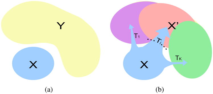
(a) The problem setting: X is the reference distribution and Y is the patient distribution. (b) Our model assumption: X is transformed into a distribution X′ covering the distribution Y, by a set of K different transformations.

The remainder of this paper is organized as follows. In section II, we explain how our clustering method CHIMERA was derived from the Coherent Point Drift algorithm [19] and how the proposed objective can be optimized in an Expectation-Maximization framework [20], [21]. The method was first validated by carrying out simulations and then used for processing two large clinical datasets (317 and 390 T1 MRI scans). The results presented in section III demonstrate the superiority of CHIMERA, compared to K-means, hierarchical clustering and two of their variations. The subtypes of AD revealed by our method using a large collection of Alzheimer's Disease MRI data are discussed in section IV, along with discussion of the merits and limitations of CHIMERA for the study of complex brain diseases.

II. Method

Let us assume that the dataset contains M normal control (NC) samples X = {x₁, …, x_m} and N patient samples Y = {y₁, …, y_N}. Let us assume that the samples are described by two sets of features: a set of D₁-dimensional imaging features: $x_m^v,y_n^v\in {\mathbb{R}}^{D_1}$; and a set of D₂-dimensional covariate features (these are known variables, such as age, sex, tumor type, treatment type): $x_m^c,y_n^c\in {\mathbb{R}}^{D_2}$. For the sake of simplicity, we will denote the samples in the compact vector forms: $x_m=(x_m^v,x_m^c)$, $y_n=(y_n^v,y_n^c)$.

We adopt a generative probabilistic framework. Considering the samples as points in the imaging space (Fig. 1), the pathology can be viewed as the difference between Y (patient) and X(NC) point distributions. Here, we model the pathological transition between the two groups as a transformation T from NC to patient distribution. When enough NC points have been collected for describing the NC population, we could assume that the estimated anatomy of patients, had they been spared of the disease, is covered by the NC distribution. Assuming that all the patients can be associated with NCs and that, conversely, the transformed NC points cover the entire set of patients, the transformation T is found by matching patient and NC distributions. Covariates are introduced into the distribution matching criteria by combining imaging and covariate-specific distances in a multi-kernel way [22].

The maximum a posteriori(MAP) optimization of the model leads to minimize the following energy ε:

$$\epsilon (\mathbf{X},\mathbf{Y},\mathrm{\Theta })=-\mathcal{L}(\mathbf{X},\mathbf{Y},\mathrm{\Theta })+\mathcal{R}(\mathrm{\Theta })$$ (1)

where Θ denotes the parameters of our model, such as transformations that are applied to X for generating Y, ℒ the log-likelihood of the distributions X and Y given the parameters and a regularization/penalty ℛ improves the stability/reliability of the estimation. These two parts are presented in detail in the next two sections.

A. Log-likelihood Term

Due to the heterogeneity of the effects of a given disease, the pathological transition might take several directions. Therefore, T consists of multiple possible transformations, each of them representing a pathological direction of imaging change. The transformed NC samples are denoted as ${\mathbf{X}}^{\prime }=[x_1^{\prime },\cdots ,x_M^{\prime }]$, where the imaging feature $x_m^v$ is transformed to $\mathbf{T}(x_m^v)$ and the covariate feature $x_m^c$ remains the same.

$$x_m^{\prime }=\mathbf{T}(x_m)=(\mathbf{T}(x_m^v),x_m^c)$$ (2)

Based on the hypothesis that the origins of patient samples are covered by the NC sample space, we assume that if we apply the pathological process to the NC samples X, the transformed NC point distribution X′ will cover the patient point distribution Y, as shown in Fig. 1(b).

The matching of distributions Y and X′ is found by a variant of Coherent Point Drift [19]. Each point $x_m^{\prime }$ is considered as a centroid of a spherical Gaussian cluster. All the clusters are assumed to have the same variance σ² that is optimized by the method. Points y_n are treated as i.i.d. data generated by a Gaussian Mixture Model (GMM) with equal weight $P(x_m^{\prime })=\frac{1}{M}$ for each cluster. The similarity between the two distribution is measured by the data likelihood of this mixture model, as presented in Equation (3).

In order to take covariate features into account, we adopt a multi-kernel setting. The distance between two points are measured by RBF kernels, where the kernel size of covariate features is r times larger than the kernel size of the imaging features. As a result, the likelihood of data Y generated by centroids X′ can be described as follows:

$$P(\mathbf{X},\mathbf{Y})=\prod _{n=1}^N\sum _{m=1}^{M}P(x_m^{\prime })P(y_n|x_m^{\prime })=\prod _{n=1}^N\sum _{m=1}^M\frac{1}{M}\frac{r^{D_2/2}}{{(\sqrt{2\pi }\sigma )}^{D_1+D_2}}·exp\{\frac{{\Vert y_n^v-\mathbf{T}(x_m^v)\Vert }^2+r{\Vert y_n^c-x_m^c\Vert }^2}{-2{\sigma }^2}\}$$ (3)

During our experiments, r was determined by the ratio of total variance of these two features.

We assume that there are K pathology directions T₁, …, T_k for a given disease. We define the transformation for one NC point to the patient space as:

$$\mathbf{T}(x_m^v)=\sum _{k=1}^K{\zeta }_{km}{T}_k(x_m^v)$$ (4)

Ideally, if the disease subtypes were distinct, ζ_km should take value 1 for the transformation corresponding to the disease subtype that affects x_m, and value 0 otherwise. In this work, we assume that patients with different pathologies might correspond to the same point in the space of NC distribution and we relax the variable ζ_km to sum up to 1 for each m. This relaxation leads us to consider the transformation T for each NC point x_m as a convex combination of all possible transformations T_k.

For the T_k, linear transformations were chosen, in order to derive analytical solutions for the distribution matching. Each T_k was described by a pair of parameters (A_k, b_k) ∈ (ℝ^D₁×D₁, ℝ^D₁):

$$\mathbf{T}(x_m^v)=\sum _{k=1}^K{\zeta }_{km}(A_k{x}_m^v+b_k)$$ (5)

where Σ_kζ_km = 1 and ζ_km ≥ 0 for all m.

During our experiments, three different kinds of A_k matrices were chosen: (1) full matrices (CHIMERA-affine), (2) diagonal matrices, in order to restrict the transformations to the combinations of scaling and translations (CHIMERA-duo) and (3) the identity, in order to consider only the translations b_k (CHIMERA-trans).

Introducing this definition of the T_k into Equation (3) leads to the following expression for the log-likelihood of the data:

$$\mathcal{L}(\mathbf{X},\mathbf{Y},\mathrm{\Theta })=\sum _{n=1}^{N}log\sum _{m=1}^M\frac{1}{M}\frac{r^{D_2/2}}{{(\sqrt{2\pi }\sigma )}^{D_1+D_2}}exp\left\{\frac{r{\Vert y_n^c-x_m^c\Vert }^2}{-2{\sigma }^2}\right\}·exp\left\{\frac{{\Vert y_n^v-{\sum }_{k=1}^K{\zeta }_{km}(A_k{x}_m^v+b_k)\Vert }^2}{-2{\sigma }^2}\right\}$$ (6)

B. Model Regularization

In an imaging feature space of dimension D₁, the dimension of parameter space of CHIMERA-affine is to the order of $\mathcal{O}(D_1^2)$, while for CHIMERA-duo and CHIMERA-trans to the order of 𝒪(D₁). In the low sample size settings that are typically observed in medical imaging studies, this large dimension yields ill posed problems. This issue is commonly mitigated by regularizing/penalizing the parameters of the transformations [23], [24]. We have adopted this approach, which improves also the generalization and the robustness of our model. In order to derive an analytical solution, we have chosen to penalize the Frobenius norm of A_k – I and the ℓ₂ norm of b_k, where I is an identity matrix. This regularization, is equivalent to posing Gaussian priors for the parameters.

$$\mathcal{R}(\mathrm{\Theta })=\frac{{\lambda }_1}{2{\sigma }^2}\sum _k{\Vert b_k\Vert }_2^2+\frac{{\lambda }_2}{2{\sigma }^2}\sum _k{\Vert A_k-\mathbf{I}\Vert }_F^2$$ (7)

Beside the explicit regularization term ℛ, our model can also be considered as being “implicitly” regularized. Instead of focusing on the points at the border between the different groups, like support vector machine [25] and relevance vector machine [26], our model always consider the entire point distributions. We aim, in that way, to reduce the sensitivity of clustering produced with respect to the individual subject variability.

The next section describes the MAP estimation strategy that was adopted for optimizing our model.

C. Optimization

In this work, we have used an Expectation-Maximization algorithm [20], [21] for optimizing the parameters Θ = (A, b, ζ, σ²) of our model, where A = {A₁, · · ·, A_K} and b = {b₁, · · ·, b_K}. The algorithm introduces latent variables z indicating the posterior probability of data point for each mixture component, $q_{nm}=q(z_n=x_m^{\prime }|y_n)$. By doing so, it provides a lower bound of the log-likelihood [21].

$${\mathcal{F}}_0=\sum _{n,m}{q}_{nm}log\left(\frac{P(y_n,x_m^{\prime })}{q_{nm}}\right)$$ (8)

The energy ε is minimized via an iterative scheme. In each iteration t, the algorithm alternates calculating the expected value of q with respect to parameter obtained in last iteration Θ^(t–1) in E-step, and updating Θ^(t) by minimizing the objective function (Equation (10)) in M-step.

During our experiments, at the initialization, the parameters σ² was set to the mean distance between dataset X and Y, ζ to be uniform distributed for each x_m, each A_k to be identity matrix I, and the translation term b_k was sampled from a normal distribution 𝒩(0, 1). The E-step and M-step were performed as follows.

E-Step

Using parameters Θ^(t–1) evaluated in previous M-step, Equation (8) was optimized at $q_{nm}=P(z_n=x_m^{\prime }|y_n)$:

$$q_{nm}=\frac{exp\left(\frac{{\Vert y_n^v-{\sum }_k{\zeta }_{km}(A_k{x}_m^v+b_k)\Vert }_2^2+r{\Vert y_n^c-x_m^c\Vert }_2^2}{-2{\sigma }^2}\right)}{{\sum }_{i=1}^{M}exp\left(\frac{{\Vert y_n^v-{\sum }_k{\zeta }_{ki}(A_k{x}_i^v+b_k)\Vert }_2^2+r{\Vert y_n^c-x_i^c\Vert }_2^2}{-2{\sigma }^2}\right)}$$ (9)

M-Step

We constructed our objective energy function ℱ(Θ) as an upper bound of our energy function ε. The minimization of ℱ(Θ) leads to the minimization of ε, which is proved in [27].

$$\mathcal{F}(\mathrm{\Theta })=\frac{1}{2{\sigma }^2}\sum _{m,n}{q}_{nm}({\Vert y_n^v-\sum _k{\zeta }_{km}(A_k{x}_m^v+b_k)\Vert }_2^2+r{\Vert y_n^c-x_m^c\Vert }_2^2)+\frac{N(D_1+D_2)}{2}log{\sigma }^2+\frac{{\lambda }_1}{2{\sigma }^2}\sum _k{\Vert b_k\Vert }_2^2+\frac{{\lambda }_2}{2{\sigma }^2}\sum _k{\Vert A_k-\mathbf{I}\Vert }_F^2$$ (10)

subject to

$$\sum _{k=1}^K{\zeta }_{km}=1\text{for}m=1,\dots ,M,0\le {\zeta }_{km}\le 1$$

The objective function is not globally convex but jointly convex in each parameter. Hence we propose an iterative procedure by minimizing the objective sequentially with respect to σ², ζ, A and b. We derived closed form solution for σ², A and b by setting derivative of objective function to zero. ζ was optimized using an advanced projected gradient descent algorithm that preserves the sum of the ζ_km [28]. The detailed parameter updating procedures are presented in Appendix A. During our experiments, we stopped the iteration when the objective difference between two iterations reached a predefined tolerance, that was set to 0.01. Because the EM algorithm only guarantees a local minimum solution, we ran the optimization several times and we kept the solution with the smallest energy value.

The next section explains how a clustering can be derived from the coefficients ζ_km and the posteriors q_nm found during the optimization, and how a new sample can be assigned to these clusters.

D. Clustering

The coefficients ζ_km can be considered as the probability, for the NC sample x_m, to undergo the transformation T_k. Let P(y_n|x_m) be the likelihood of a patient sample y_n to be associated with x_m. Then, the likelihood of a given patient sample, y_n, to have been generated by the transformation T_k can be estimated by:

$$P_k(y_n)=\sum _{m}P(y_n|x_m){\zeta }_{km}$$ (11)

Because the posteriors q_nm are proportional to P(y_n|x_m), with a common denominator for each n (Equation (9)), they can be used for partitioning the patient samples according to their main transformation, by choosing for each patient y_n the label l_n corresponding to the largest likelihood:

$$l_n=\underset{k}{\text{argmax}}{P}_k(y_n)=\underset{k}{\text{argmax}}\sum _m{q}_{nm}{\zeta }_{km}$$ (12)

As long as the ζ_km are stored, the label can be estimated for a novel data s by: (1) computing the likelihood P(s|x_m) based on distances between the novel sample s and the transformed controls X′, (2) computing P_k(s) and obtaining the label l_s = argmax_k P_k(s). This strategy was adopted for clustering clinical data during our experiments.

III. Experiments and Results

This section presents the experiments that were conducted for validating our approach. We compared first our approach with two standard clustering methods, K-means [15] and hierarchical Ward clustering [17], and two variants of these methods, on synthetic data and a real dataset of dementia patients with known subtypes. The promising results obtained incited us to analyze a clinical dataset where the ground truth is unknown.

We used CHIMERA for clustering a population of AD patients extracted from the ADNI dataset¹. Our analysis revealed two stable/reproducible subtypes that are strongly specific of AD according to prior clinical studies, while exhibiting distinct imaging patterns and clinical profiles, as if they were corresponding to distinct pathological trajectories. Detailed investigations that are outside the scope of this paper will be carried out in the future for elucidating all the medical implications of this finding.

A. Simulated Data

Our method was first validated using synthetic data simulating the effect of age and disease on brain volume.

The brain was divided into 20 regions (ROIs), where the atrophy was described by a normalized volume between 0 (the most serious atrophy) and 1 (largest possible ROI volume).

The simulated data was generated as follows:

1. 1000 samples were generated independently. For each sample, 20 ROI volumes were sampled randomly from a normal distribution, 𝒩(1, 0.1). In addition, each sample was associated with a random age, sampled from a uniform distribution between 55 and 85.

2. Age effect was introduced for each ROI volume and every sample, by subtracting the atrophy volume. The ROI volume atrophy was simulated by a normal distribution 𝒩(0.01(t – 55), 0.005(t – 55)), where t is the age. This simulation corresponds to a linear volume decrease with age of slope 0.01 per year; and a variance increase of slope 0.005 per year.

3. The samples were randomly separated into two 500-sample groups, a control group and a patient group. The patient group was further divided into two sub-groups of 250 samples. In each patient group we introduced an atrophy pattern induced by a 15% decrease in volume in pre-selected regions. Some of the regions selected were common across the subgroups while some others were distinct. This was done to simulate the effect of two distinct but overlaping variants of a same neurodegenerative disease. The two atrophy patterns are presented in Fig. 2.

4. The ROIs volumes were then normalized independently, by scaling them between 0 (the most atrophied sample ROI volume) and 1 (the largest sample ROI volume).

Fig. 2. Atrophy patterns introduced (in red).

The simulated data with age effect is plotted in Fig. 3. For both groups, the normalized total volume decreases as age increases. Patient group has smaller total volume due to the disease effect. But as the variance increases, the disease effect is overwhelmed by the age effect.

Fig. 3.

Simulated age effect on the normalized total volume. As age increase, the total volume linearly decreases and the variance of the ROI volumes increases.

We compared our model with K-means [15] clustering and Ward hierarchical clustering [17]. However, standard clustering methods do not have access to the information of control group as CHIMERA does. For fair comparison, we considered therefore two supplementary variants of these clustering methods. Similar to pattern-based morphometry [29], we computed a “profile” for each patient subject: we computed the difference vector between each patient point and its Euclidean nearest neighbor in the control group. These profiles were clustered instead of the original patient data. In these analysis, a general linear regression(GLM) [30] was performed on the imaging features for removing the age effects prior to the clustering. The three variants of our method were applied to the synthetic data. We set model parameters as follows, CHIMERA-affine: (λ₁, λ₂) = (10,100); CHIMERA-duo: (λ₁, λ₂) = (10,10); CHIMERA-trans: λ₁ = 10.

The simulation was repeated 100 times independently. All the methods were applied on each simulated data set, with K = 2. The Dice score [31] of overlap between the ground truth and the clustering labels were generated for each run, and the box plots for different methods are presented in Fig. 4. Given that the dice score is 0.5 when the labels are assigned randomly, our method performs better than clustering methods and their profile-based variations. CHIMERA-duo outperformed the other CHIMERA variants. This result indicates that CHIMERA-duo model contains enough degrees of freedom for capturing the differences between patient and control groups that cannot be expressed as a pure translation. In the meantime, the model is much smaller than the affine model, that is hard to regularize.

Fig. 4.

Box plot of dice scores on synthetic data between ground truth labels and outputs of clustering methods: (a) K-means, (b) K-means with profile, (c) Hierarchical clustering, (d) Hierarchical clustering with profile, (e) CHIMERA-affine, (f) CHIMERA-duo and (g) CHIMERA-trans.

B. Dementia Dataset

Before using our method for exploring unknown heterogeneous imaging patterns, we validated our approach on a dementia dataset containing patients suffering from different diseases generating distinct imaging patterns. We used a dementia clinical dataset of 317 T1 structural MRI scans corresponding to 148 Alzheimer's Disease (AD) patients, 91 Parkinson's Disease (PD) patients and 78 Normal Controls (NC). The images were skull-stripped, co-registered and Multi-Atlas ROIs were generated [32] [33]. The volumes of 80 ROIs were calculated, as well as the volume of brain lesions that they contain [34]. Age and gender of each subject were utilized as covariate features.

The performances of the seven methods described in section III-A were estimated by performing one hundred 10-folds cross-validations on the dataset. For each cross-validation, the patient samples were partitioned randomly into 10 folds. For each fold, the clustering was first established by using normal control samples and the remaining 90% patients. The 10% test samples of the fold were then assigned clustering labels. For K-means and Hierarchical clustering, the assignment was based on the distance to cluster centers; for our approach, the assignment procedure is explained in section II-D. After this assignment, the dice score between the known subtype labels and the labels produced by the clustering methods was computed for the samples of the fold. A dice score for the entire cross-validation was obtained by averaging the dice scores obtained for the ten folds. Running the cross-validation one hundred time with different partitions of the patient data produced the distribution of dice scores shown in Fig. 5. There is a significant performance gap between our approach and standard clustering methods. CHIMERA-duo and CHIMERA-trans worked comparably well, while the performance of the CHIMERA-affine model were a little lower.

Fig. 5.

Box plot of dice scores on dementia dataset between ground truth labels and outputs of clustering methods: (a) K-means, (b) K-means with profile, (c) Hierarchical clustering, (d) Hierarchical clustering with profile, (e) CHIMERA-affine, (f) CHIMERA-duo and (g) CHIMERA-trans.

This experiment confirms that our approach can identify distinct imaging patterns corresponding to clinically heterogeneous populations using real imaging data. We finally used CHIMERA for investigating the existence of subtypes of Alzheimer's Disease. We used CHIMERA-duo for this task, because this variant has the best trade-off between model complexity and generalization performances.

C. Alzheimer's Disease Dataset

We analyze the heterogeneity of Alzheimer's Disease by applying CHIMERA-duo to ADNI dataset of 390 T1 structural MRI scans with 177 AD patients and 213 Normal Controls. Similar to the preprocessing in section III-B, the volumes of 80 ROIs were calculated. Age and gender information were utilized as covariate features.

The model parameters, K (number of sub-clusters) and λ₁, λ₂ (parameters of the regularization term), were selected according to the reproducibility and data fit of the clustering outputs. We observed that when the ratio between λ₁ and λ₂ is too large, the transformations are relatively unconstrained, which leads to poor convergence. Small ratio, on the contrary, let the transformation degenerate into a pure translation, which is not desirable either. We empirically fixed this ratio as follows: λ₁ = λ₂ = λ.

The reproducibility was measured by the Adjusted Rand Index(ARI) [35] (Appendix B), which were extensively cross-validated. We ran experiments for K = 2, 3, 4 clusters, λ = 5, 7, …, 31 and 35. For each combination of K and λ, 100 runs of leave-10%-out clusterings were performed. During each clustering, a random subset of 90% of the patient samples and all the normal control samples were used for generating the transformations and defining the patient clusters. The remaining 10% patient samples were assigned to the group found, based on their proximity with the transformed control, as explained in the section II-D.

We measured the ARI between all the pairs of the 100 clusterings obtained for each parameter value, and averaged the ARI for each clustering. The complete results are shown in Fig. 6. When K increases, more transformation parameters are required (2KD₁). Small λs lead to ill-conditioned optimization that do not converge. This is for instance the case when λ < 11 and K = 4. On the other hand, large λ result in null/small transformations that are close to the identity, which is not desirable. For these reasons, smaller λ are preferable when the reproducibilities are comparable.

Fig. 6.

Reproducibility measured by the average Adjusted Rand Index [35], for all the number of cluster K tested, and all the sparsity parameter λ. The median average ARI corresponding to a same K were connected for improving the visualization of the trends.

We finally selected (K = 2, λ = 15), a set of parameters corresponding to a high reproducibility for a reasonable good data fit. In order to analyze the subtypes found by our method in detail, we selected the clustering providing the highest sum of ARI with the other clusterings, among the hundred clusterings associated with this set of parameters. This clustering is the medoid of the clusterings produced, and therefore the most reliable.

In this clustering, 177 AD patients are clustered into two subgroups: subgroup 1 with 91 subjects and subgroup 2 with 86 subjects. In order to reveal detailed disease signatures, we performed ROI-wise t-test for each subgroup against the control group, as well as the subgroups against each other. In Fig. 7, the t-stats for the ROIs are displayed in a heat map, thresholded at level of FDR adjusted p-value 0.01. Red color indicates when the first group has more volume than the last group. The opposite is indicated with blue color. The correspondence between the ROIs' names and labels is displayed in Table I [33].

Fig. 7.

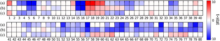
ROI-wise t-test results of: (a) Subgroup 1 v.s. Control group, (b) Subgroup 2 v.s. Control group, (c) Subgroup 1 v.s. Subgroup 2, for all the 80 ROIs. The t-stats thresholded by FDR adjusted p-value at level of 0.01 for the ROIs are shown. Red color indicates when the first group has more volume than the last group. The opposite is indicated with blue color. The names of these ROIs are displayed in Table I.

Table I. Names of 80 ROIs^1,2.

#	Name	#	Name
1	3rd Ventricle	41	Parietal Lobe WM L
2	4th Ventricle	42	Temporal Lobe WM R
3	Accumbens Area R	43	Temporal Lobe WM L
4	Accumbens Area L	44	Fornix R
5	Amygdala R	45	Fornix L
6	Amygdala L	46	Anterior Limb Intern. Capsule R
7	Brain Stem	47	Anterior Limb Intern. Capsule L
8	Caudate R	48	Posterior Limb Intern. Capsule R
9	Caudate L	49	Posterior Limb Intern. Capsule L
10	Cerebellum Exterior R	50	Corpus Callosum
11	Cerebellum Exterior L	51	Frontal Inferior GM L
12	Cerebellum WM R	52	Frontal Insular GM L
13	Cerebellum WM L	53	Frontal Lateral GM L
14	CSF	54	Frontal Medial GM L
15	Hippocampus R	55	Frontal Opercular GM L
16	Hippocampus L	56	Limbic Cingulate GM L
17	Inf Lat Vent R	57	Limbic Medialtemporal GM L
18	Inf Lat Vent L	58	Occipital Inferior GM L
19	Lateral Ventricle R	59	Occipital Lateral GM L
20	Lateral Ventricle L	60	Occipital Medial GM L
21	Pallidum R	61	Parietal Lateral GM L
22	Pallidum L	62	Parietal Medial GM L
23	Putamen R	63	Temporal Inferior GM L
24	Putamen L	64	Temporal Lateral GM L
25	Thalamus Proper R	65	Temporal Supratemporal GM L
26	Thalamus Proper L	66	Frontal Inferior GM R
27	Ventral DC R	67	Frontal Insular GM R
28	Ventral DC L	68	Frontal Lateral GM R
29	Vessel R	69	Frontal Medial GM R
30	Vessel L	70	Frontal Opercular GM R
31	Cere. Vermal Lob. 1-5	71	Limbic Cingulate GM R
32	Cere. Vermal Lob. 6-7	72	Limbic Medialtemporal GM R
33	Cere. Vermal Lob. 8-10	73	Occipital Inferior GM R
34	Basal Forebrain L	74	Occipital Lateral GM R
35	Basal Forebrain R	75	Occipital Medial GM R
36	Frontal Lobe WM R	76	Parietal Lateral GM R
37	Frontal Lobe WM L	77	Parietal Medial GM R
38	Occipital Lobe WM R	78	Temporal Inferior GM R
39	Occipital Lobe WM L	79	Temporal Lateral GM R
40	Parietal Lobe WM R	80	Temporal Supratemporal GM R

¹GM: gray matter; WM: white matter; R: right; L: left.

²The ROIs are extracted as in Doshi et al. [33].

As shown in Fig. 7 row (a) and (b), both patient subgroups present brain volume loss compared to normal controls, in regions including the temporal and limbic lobe, which are typical atrophy regions observed in Alzheimer's disease [36]–[39]. Also, both subgroups have larger ventricle volumes as compared to the control group. However, as shown in row (c), these two subgroups present significant between group differences in the following regions:

1. Subgroup 1 has more gray matter atrophy in limbic lobe including amygdala and hippocampus (5,6,15,16), and frontal insular regions (52,67). This atrophy pattern has been related to AD by many clinical studies, such as [39].

2. Subgroup 2 exhibits unique parietal and occipital gray matter atrophy on both lateral and medial structures (59-62,74-77). These atrophy patterns have also previously been noted in the literature [38]–[40]. Some reports have linked posterior cingulate and precuneous atrophy to early onset AD [41], [42].

3. Subgroup 1 exhibits unique deep gray matter atrophy in basal ganglia (3,4,8,9,21-24), a region that was also related to AD, for instance by Teipel et al. [43].

We performed a Voxel-Based Morphometry [44] on gray matter for each subgroup against the control group using the RAVENS maps that were generated during the co-registration [32]. RAVENS maps measure the tissue density of a brain with respect to a template [45], [46]. The t-stats map thresholded by FDR adjusted p-value 0.01 are presented in Fig. 8. We have circled out the significant different regions as discussed.

Fig. 8.

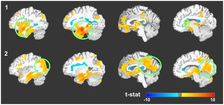
Voxel-based Morphometry [5] performed on gray matter RAVENS maps [45] between (1) Subgroup 1 and Control group; (2) Subgroup 2 and Control group. The t-stats, thresholded by FDR adjusted p-value at level of 0.01 are presented, overlaid on the registration template image. Red color indicates volume loss and blue color volume increase. The green circles highlight the differences between the subgroups.

A statistical analysis was carried out for determining if the two subgroups exhibit different clinical cognitive performance. We used MMSE score [47], ADAS-cog 11 score and ADAS-cog 13 score in this analysis. The score distributions, that are not Gaussian, were compared by a rank sum test [48]. The results are displayed in Table II. The subgroup 1 performed significantly worse than subgroup 2 in ADAS-cog test. The difference is less noticeable for the MMSE test. We performed a rank sum test for comparing the age distribution in the two groups. Subgroup 1 appeared to be slightly older than subgroup 2, but the test does not reach significance at the α = 0.05 level.

Table II. Cognitive score difference between the subgroups.

	MMSE	ADAS-cog 11	ADAS-cog 13
Mean difference1	−0.5284	1.9454	2.5913
p-value2	0.0787	0.0144	0.0183

¹Score mean of subgroup 1 subtracted by that of subgroup 2

²p-value is based on Ranksum test.

These findings indicate that our method has extracted distinct patterns of atrophy that have been previously implicated in Alzheimer's disease. Interestingly, the posterior cingulate/precuneous atrophy has been previously hypothesized to relate to early rather than late onset AD [41], which might imply that our identified 2 clusters also differentiate early vs. late onset patients.

IV. Discussion

We have proposed a new approach, CHIMERA, for identifying disease subtypes of heterogeneous diseases. Our approach relies on a point distribution mapping, while allowing the to reduction of the influence of nuisance covariates. The approach adopted overcomes several methodological limitations of existing methods for the analysis of disease heterogeneity. We discuss here three main aspects that have not been presented in detail in the previous sections. We also discuss a way to address the main limitation of our current framework.

First, the soft assignment performed by our model provides a rich information about the pathology. Each normal/control point is transformed with a probability distribution ζ by all possible transformations. This notion implies that a healthy subject might transition to a diseased state via various pathological patterns/processes. The clustering of patients is based on the posterior probability q and ζ. Instead of a hard assignment for clustering outputs, our approach produces probability soft assignment which might better describe the disease effects.

Second, the framework is modular. In this work, we have used a linear transformation with scaling and translation that has 𝒪(D) degrees of freedom. Since the sample sizes of most neuroimaging studies are relatively small, we might improve the performance of the model by choosing a more constrained transformation. For instance, the transformation could be represented by the displacement of a few reference samples [19]. Such transformation would exhibit much fewer degrees of freedom, which would improve the robustness of the optimization/clustering. Hierarchical transformations could also be implemented, similarly to [32], for reducing the computational burden and/or better constraining the transformation.

Thirdly, we integrate the covariate features in a multi-kernel way. Our framework does not make explicit assumption on the effect of covariates where GLM assumes that covariates have a linear relationship with the imaging features. With this strategy, our framework mitigates the effect of covariates softly, rather than a hard threshold in stratification which is an alternate way of solving this issue.

The large dimension of the transformations involved in our current framework constitutes its main limitation. The optimization instability induced was partially addressed by penalizing the transformations. However, this approach would not be suitable for high dimensional data such as voxel-level image maps [45] or voxel-wise transformations. The use of sparser transformations, as explained above, will help reducing the dimension of our model. Stricter penalties, such as ℓ₂₁ and ℓ₁ penalties, can be investigated in the future. However, we think that dimensionality reduction will probably remain necessary, in order to maintain the stability of the optimization and reduce the number of local optima. Another limitation of our current linear transformation formulation is that it doesn't take into account the covariance structure of the data, such as covariation between left and right side of the brain. Though we already got symmetric results in Fig. 7, it might be beneficial to introduce this constraint into the framework. Lastly, the Euclidean distance adopted in the framework implicitly treats features with the same weight. This limitation could be addressed by introducing Mahalanobis distance. These aspects will be further investigated in the future.

V. Conclusion

In this paper, we have presented a novel clustering framework, CHIMERA, that addresses some of the challenges raised by the heterogeneity of many diseases, especially neurodegenerative and neuropsychiatric diseases. In our approach, patients and controls are treated as point distributions and disease effects are represented by a set of transformations applied to them, each transformation standing for a different pathology subtype. Another critical contribution of our work is the integration of covariates. Our framework performs a matching between patients and controls based on these covariates in addition to the imaging features, by combining multiple distance/kernels. This matching mitigates potentially confounding effects of covariates that might not be relevant to the disease effect.

CHIMERA was validated on simulated data and on a clinical dataset where different dementia were mixed. The promising results obtained incited us to explore the heterogeneity of a patient group extracted from the ADNI database. CHIMERA recognized two patient groups, corresponding to distinct pathological brain atrophy patterns. These groups were found to present distinct cognitive abilities. This result illustrates the potential of our method for helping to refine the phenotyping of neurodegenerative diseases, and could potentially reflect early vs. late onset AD subtypes.

Appendix A

Optimization M-step Details

With the following notations:

• ${\mathbf{X}}_v^{\prime }$: D₁ × M matrix, mth column is $\mathbf{T}(x_m^v)$

• X_c : D₂ × M matrix, mth column is $x_m^c$

• Y_v : D₁ × N matrix, nth column is $y_n^v$

• Y_c : D₂ × N matrix, nth column is $y_n^c$

• ζ : K × M matrix, [ζ]_km = ζ_km, ith row is ζ_i·, mth column is ζ_·m

• Q : N × M matrix, [Q]_nm = q_nm

• d(u) : matrix with its diagonal elements from vector u

• d⁻¹(U) : vector contains diagonal elements of matrix U

• tr(U) : trace of matrix U

• 1 : column vector with all elements to be 1

• ○ : element-wise division

For each i = 1, …, K:

• ${\mathbf{X}}_1^i$ : D₁ × M matrix, mth column is ${\sum }_{k\ne i}{\zeta }_{km}(A_k{x}_m^v+b_k)$

• ${\mathbf{X}}_2^i$ : D₁ × M matrix, mth column is ${\zeta }_{im}{x}_m^v$

• ${\mathbf{X}}_3^i$ : D₁ × M matrix, mth column is ${\zeta }_{im}^2{x}_m^v$

• ${\mathbf{X}}_4^i$ : D₁ × M matrix, mth column is $A_i{x}_m^v$

1. The updating rule for σ² is:

   $$\begin{gathered} {\sigma }^2=[\text{tr}({\mathbf{Y}}_v\mathrm{d}(\mathbf{Q}\mathbf{1}){\mathbf{Y}}_v^T-2{\mathbf{Y}}_v\mathbf{Q}{\mathbf{X}}_v^{\prime T}+{\mathbf{X}}_v^{\prime }\mathrm{d}({\mathbf{Q}}^T\mathbf{1}){\mathbf{X}}_v^{\prime T}) \\ +\text{tr}({\mathbf{Y}}_c\mathrm{d}(\mathbf{Q}\mathbf{1}){\mathbf{Y}}_c^T-2{\mathbf{Y}}_c\mathbf{Q}{\mathbf{X}}_c^T+{\mathbf{X}}_c\mathrm{d}({\mathbf{Q}}^T\mathbf{1}){\mathbf{X}}_c^T) \\ +{\lambda }_1\sum _k{\Vert b_k\Vert }_2^2+{\lambda }_2\sum _k{\Vert A_k-\mathbf{I}\Vert }_F^2]/N(D_1+D_2) \end{gathered}$$ (13)

2. The updating rule for each A_i, i = 1 · · · K, When A_i is arbitrary matrix:

   $$A_i=({\mathbf{Y}}_v\mathbf{Q}{\mathbf{X}}_2^{iT}-{\mathbf{X}}_1^i\mathrm{d}({\mathbf{Q}}^T\mathbf{1}){\mathbf{X}}_2^{iT}-b_i{\mathbf{1}}^T\mathbf{Q}{\mathbf{X}}_3^{iT}+{\lambda }_2\mathbf{I}){({\mathbf{X}}_2^i\mathrm{d}({\mathbf{Q}}^T\mathbf{1}){\mathbf{X}}_2^{iT}+{\lambda }_2\mathbf{I})}^{-1}$$ (14)

   When A_i is diagonal matrix:

   $$A_i=\mathrm{d}[{\mathrm{d}}^{-1}({\mathbf{Y}}_v\mathbf{Q}{\mathbf{X}}_2^{iT}-{\mathbf{X}}_1^i\mathrm{d}({\mathbf{Q}}^T\mathbf{1}){\mathbf{X}}_2^{iT}-b_i{\mathbf{1}}^T\mathbf{Q}{\mathbf{X}}_3^{iT}+{\lambda }_2\mathbf{I})\circ ({\mathrm{d}}^{-1}({\mathbf{X}}_2^i\mathrm{d}({\mathbf{Q}}^T\mathbf{1}){\mathbf{X}}_2^{iT}+{\lambda }_2\mathbf{I}))]$$ (15)

   When A_i is identity matrix, skip optimizing for A.

3. The updating rule for each b_i, i = 1 · · · K is:

   $$b_i=\frac{{\mathbf{Y}}_v\mathrm{d}(\mathbf{Q}{\zeta }_i^T)\mathbf{1}-{\mathbf{X}}_1^i\mathrm{d}({\zeta }_{i·}){\mathbf{Q}}^T\mathbf{1}-{\mathbf{X}}_4^i\mathrm{d}{({\zeta }_{i·})}^2{\mathbf{Q}}^T\mathbf{1}}{{\mathbf{1}}^T\mathbf{Q}\mathrm{d}({\zeta }_i){\zeta }_i^T+{\lambda }_1}$$ (16)

4. To update ζ_·m, we use a projected gradient descent scheme. First we move ζ_im for i = 1, · · ·, K with Newton's method:

   $$\begin{array}{c}\frac{\partial \mathcal{F}}{\partial {\zeta }_{im}}=\frac{1}{{\sigma }^2}\sum _n{q}_{nm}{(y_n^v-\sum _k{\zeta }_{km}(A_k{x}_m^v+b_k))}^T(-A_i{x}_m^v-b_i)\\ \frac{{\partial }^2\mathcal{F}}{\partial {\zeta }_{im}^2}=\frac{1}{{\sigma }^2}\sum _n{q}_{nm}{(A_k{x}_m^v+b_k)}^T(A_i{x}_m^v-b_i)\\ {\zeta }_{im}^{\mathit{\text{new}}}={\zeta }_{im}^{\mathit{\text{old}}}-\frac{\partial \mathcal{F}}{\partial {\zeta }_{im}}·{\left(\frac{{\partial }^2\mathcal{F}}{\partial {\zeta }_{im}^2}\right)}^{-1}\end{array}$$

   Then we projected the new vector ${\zeta }_{·m}^{\mathit{\text{new}}}$ back to the feasible set (ℓ₁ simplex) using method proposed in [28].

Appendix B

Definition of Adjusted Rand Index

The Adjusted Rand Index was proposed by Hubert and Arabie [35]. Suppose that a set of sample was labeled/clustered twice, and let denote the two labelings with X = {x}, Y = {y}. The matrix m_x,y = |x∩y| is defined, where |x∩y| is the number of subjects labeled x in X and y in Y. With the following notations a_x = Σ_ym_x,y and b_y = Σ_xm_x,y, the Adjusted Rand Index(ARI) is calculated as:

$$\text{ARI}=\frac{{\sum }_{x,y}\left(\begin{array}{c}{m}_{x,y}\\ 2\end{array}\right)-\left[{\sum }_x\right(\begin{array}{c}{a}_x\\ 2\end{array}\left){\sum }_y\right(\begin{array}{c}{b}_y\\ 2\end{array}\left)\right]/\left(\begin{array}{c}N\\ 2\end{array}\right)}{\frac{1}{2}\left[{\sum }_x\right(\begin{array}{c}{a}_x\\ 2\end{array})+{\sum }_y(\begin{array}{c}{b}_y\\ 2\end{array}\left)\right]-\left[{\sum }_x\right(\begin{array}{c}{a}_x\\ 2\end{array}\left){\sum }_y\right(\begin{array}{c}{b}_y\\ 2\end{array}\left)\right]/\left(\begin{array}{c}N\\ 2\end{array}\right)}$$

References

- 1.Yamasue H, Kasai K, Iwanami A, Ohtani T, Yamada H, Abe O, Kuroki N, Fukuda R, Tochigi M, Furukawa S, et al. Voxel-based analysis of MRI reveals anterior cingulate gray-matter volume reduction in posttraumatic stress disorder due to terrorism. Proceedings of the National Academy of Sciences. 2003;100(151):9039–9043. doi: 10.1073/pnas.1530467100. [DOI] [PMC free article] [PubMed] [Google Scholar]
- 2.Good CD, Johnsrude IS, Ashburner J, Henson RN, Friston KJ, Frackowiak RS. A Voxel-Based Morphometric Study of Ageing in 465 Normal Adult Human Brains. NeuroImage. 2001;14(1):21–36. doi: 10.1006/nimg.2001.0786. [DOI] [PubMed] [Google Scholar]
- 3.Giedd JN, Blumenthal J, Jeffries NO, Castellanos FX, Liu H, Zijdenbos A, Paus T, Evans AC, Rapoport Jl. Brain development during childhood and adolescence: a longitudinal MRI study. Nature neuroscience. 1999;2(10):861–863. doi: 10.1038/13158. [DOI] [PubMed] [Google Scholar]
- 4.Thirion B, Pinel P, Mériaux S, Roche A, Dehaene S, Poline JB. Analysis of a large fMRI cohort: Statistical and methodological issues for group analyses. Neuroimage. 2007;35(1):105–120. doi: 10.1016/j.neuroimage.2006.11.054. [DOI] [PubMed] [Google Scholar]
- 5.Ashburner J, Friston KJ. Voxel-based morphometrythe methods. Neuroimage. 2000;11(6):805–821. doi: 10.1006/nimg.2000.0582. [DOI] [PubMed] [Google Scholar]
- 6.Davatzikos C, Genc A, Xu D, Resnick SM. Voxel-based morphometry using the RAVENS maps: methods and validation using simulated longitudinal atrophy. NeuroImage. 2001;14(6):1361–1369. doi: 10.1006/nimg.2001.0937. [DOI] [PubMed] [Google Scholar]
- 7.Honea R, Crow TJ, Passingham D, Mackay CE. Regional deficits in brain volume in schizophrenia: a meta-analysis of voxel-based morphometry studies. 2014 doi: 10.1176/appi.ajp.162.12.2233. [DOI] [PubMed] [Google Scholar]
- 8.Goodlett CB, Fletcher PT, Gilmore JH, Gerig G. Group analysis of DTI fiber tract statistics with application to neurodevelopment. NeuroImage. 2009;45(1):S133–S142. doi: 10.1016/j.neuroimage.2008.10.060. [DOI] [PMC free article] [PubMed] [Google Scholar]
- 9.Murray ME, Graff-Radford NR, Ross OA, Petersen RC, Duara R, Dickson DW. Neuropathologically defined subtypes of Alzheimer's disease with distinct clinical characteristics: a retrospective study. The Lancet Neurology. 2011;10(9):785–796. doi: 10.1016/S1474-4422(11)70156-9. [DOI] [PMC free article] [PubMed] [Google Scholar]
- 10.Fenton WS, McGlashan TH, Victor BJ, Blyler CR. Symptoms, subtype, and suicidality in patients with schizophrenia spectrum disorders. American journal of psychiatry. 1997;154(2):199–204. doi: 10.1176/ajp.154.2.199. [DOI] [PubMed] [Google Scholar]
- 11.Tager-Flusberg H, Joseph RM. Identifying neurocognitive phenotypes in autism. Philosophical Transactions of the Royal Society B: Biological Sciences. 2003;358(1430):303–314. doi: 10.1098/rstb.2002.1198. [DOI] [PMC free article] [PubMed] [Google Scholar]
- 12.Wåhlstedt C, Thorell LB, Bohlin G. Heterogeneity in adhd: neuropsychological pathways, comorbidity and symptom domains. Journal of abnormal child psychology. 2009;37(4):551–564. doi: 10.1007/s10802-008-9286-9. [DOI] [PubMed] [Google Scholar]
- 13.Marusyk A, Polyak K. Tumor heterogeneity: causes and consequences. Biochimica et Biophysica Acta (BBA)-Reviews on Cancer. 2010;1805(1):105–117. doi: 10.1016/j.bbcan.2009.11.002. [DOI] [PMC free article] [PubMed] [Google Scholar]
- 14.Garcia-Closas M, Hall P, Nevanlinna H, Pooley K, Morrison J, Richesson DA, Bojesen SE, Nordestgaard BG, Axelsson CK, Arias JI, et al. Heterogeneity of breast cancer associations with five susceptibility loci by clinical and pathological characteristics. PLoS genetics. 2008;4(4):e1000054. doi: 10.1371/journal.pgen.1000054. [DOI] [PMC free article] [PubMed] [Google Scholar]
- 15.Lloyd S. Least squares quantization in PCM. Information Theory, IEEE Transactions on. 1982;28(2):129–137. [Google Scholar]
- 16.Johnson SC. Hierarchical clustering schemes. Psychometrika. 1967;32(3):241–254. doi: 10.1007/BF02289588. [DOI] [PubMed] [Google Scholar]
- 17.Ward JH., Jr Hierarchical grouping to optimize an objective function. Journal of the American statistical association. 1963;58(301):236–244. [Google Scholar]
- 18.Noh Y, Jeon S, Lee JM, Seo SW, Kim GH, Cho H, Ye BS, Yoon CW, Kim HJ, Chin J, et al. Anatomical heterogeneity of Alzheimer disease Based on cortical thickness on MRIs. Neurology. 2014;83(21):1936–1944. doi: 10.1212/WNL.0000000000001003. [DOI] [PMC free article] [PubMed] [Google Scholar]
- 19.Myronenko A, Song X. Point set registration: Coherent point drift. PAMI. 2010;32:2262–2275. doi: 10.1109/TPAMI.2010.46. [DOI] [PubMed] [Google Scholar]
- 20.Moon TK. The expectation-maximization algorithm. Signal processing magazine, IEEE. 1996;13(6):47–60. [Google Scholar]
- 21.Bishop C, et al. Pattern recognition and machine learning. Vol. 1 springer; New York: 2006. [Google Scholar]
- 22.Lanckriet GR, Cristianini N, Bartlett P, Ghaoui LE, Jordan MI. Learning the kernel matrix with semidefinite programming. The Journal of Machine Learning Research. 2004;5:27–72. [Google Scholar]
- 23.Schölkopf B, Smola AJ. Learning with kernels: Support vector machines, regularization, optimization, and beyond. MIT press; 2002. [Google Scholar]
- 24.Engl HW, Hanke M, Neubauer A. Regularization of inverse problems. Vol. 375 Springer Science & Business Media; 1996. [Google Scholar]
- 25.Cortes C, Vapnik V. Support-vector networks. Machine learning. 1995;20(3):273–297. [Google Scholar]
- 26.Tipping ME. Sparse Bayesian learning and the relevance vector machine. The journal of machine learning research. 2001;1:211–244. [Google Scholar]
- 27.Neal RM, Hinton GE. Learning in graphical models. Springer; 1998. A view of the EM algorithm that justifies incremental, sparse, and other variants; pp. 355–368. [Google Scholar]
- 28.Duchi J, Shalev-Shwartz S, Singer Y, Chandra T. Proceedings of the 25th international conference on Machine learning. ACM; 2008. Efficient projections onto the l 1-ball for learning in high dimensions; pp. 272–279. [Google Scholar]
- 29.Gaonkar B, Pohl K, Davatzikos C. Medical Image Computing and Computer-Assisted Intervention–MICCAI 2011. Springer; 2011. Pattern based morphometry; pp. 459–466. [DOI] [PMC free article] [PubMed] [Google Scholar]
- 30.McCullagh P. Generalized linear models. European Journal of Operational Research. 1984;16(3):285–292. [Google Scholar]
- 31.Dice LR. Measures of the amount of ecologic association between species. Ecology. 1945;26(3):297–302. [Google Scholar]
- 32.Ou Y, Sotiras A, Paragios N, Davatzikos C. DRAMMS: De-formable registration via attribute matching and mutual-saliency weighting. Medical image analysis. 2011;15(4):622–639. doi: 10.1016/j.media.2010.07.002. [DOI] [PMC free article] [PubMed] [Google Scholar]
- 33.Doshi J, Erus G, Ou Y, Gaonkar B, Davatzikos C. Multi-atlas skull-stripping. Academic radiology. 2013;20(12):1566–1576. doi: 10.1016/j.acra.2013.09.010. [DOI] [PMC free article] [PubMed] [Google Scholar]
- 34.Lao Z, Shen D, Liu D, Jawad AF, Melhem ER, Launer LJ, Bryan RN, Davatzikos C. Computer-assisted segmentation of white matter lesions in 3D MR images using support vector machine. Academic radiology. 2008;15(3):300–313. doi: 10.1016/j.acra.2007.10.012. [DOI] [PMC free article] [PubMed] [Google Scholar]
- 35.Hubert L, Arabie P. Comparing partitions. Journal of classification. 1985;2(1):193–218. [Google Scholar]
- 36.Fox N, Warrington E, Freeborough P, Hartikainen P, Kennedy A, Stevens J, Rossor MN. Presymptomatic hippocampal atrophy in Alzheimer's disease A longitudinal MRI study. Brain. 1996;119(6):2001–2007. doi: 10.1093/brain/119.6.2001. [DOI] [PubMed] [Google Scholar]
- 37.Thompson PM, Hayashi KM, De Zubicaray G, Janke AL, Rose SE, Semple J, Herman D, Hong MS, Dittmer SS, Doddrell DM, et al. Dynamics of gray matter loss in Alzheimer's disease. The Journal of Neuroscience. 2003;23(3):994–1005. doi: 10.1523/JNEUROSCI.23-03-00994.2003. [DOI] [PMC free article] [PubMed] [Google Scholar]
- 38.Karas G, Scheltens P, Rombouts S, Visser P, Van Schijndel R, Fox N, Barkhof F. Global and local gray matter loss in mild cognitive impairment and alzheimer's disease. Neuroimage. 2004;23(2):708–716. doi: 10.1016/j.neuroimage.2004.07.006. [DOI] [PubMed] [Google Scholar]
- 39.Foundas AL, Leonard CM, Mahoney SM, Agee OF, Heilman KM. Atrophy of the hippocampus, parietal cortex, and insula in alzheimer's disease: a volumetric magnetic resonance imaging study. Cognitive and Behavioral Neurology. 1997;10(2):81–89. [PubMed] [Google Scholar]
- 40.Holroyd S, Shepherd ML, Downs JH., III Occipital atrophy is associated with visual hallucinations in alzheimer's disease. The Journal of neuropsychiatry and clinical neurosciences. 2000 doi: 10.1176/jnp.12.1.25. [DOI] [PubMed] [Google Scholar]
- 41.Karas G, Scheltens P, Rombouts S, van Schijndel R, Klein M, Jones B, van der Flier W, Vrenken H, Barkhof F. Precuneus atrophy in early-onset alzheimers disease: a morphometric structural mri study. Neuroradiology. 2007;49(12):967–976. doi: 10.1007/s00234-007-0269-2. [DOI] [PubMed] [Google Scholar]
- 42.Shima K, Matsunari I, Samuraki M, Chen WP, Yanase D, Noguchi-Shinohara M, Takeda N, Ono K, Yoshita M, Miyazaki Y, et al. Posterior cingulate atrophy and metabolic decline in early stage alzheimer's disease. Neurobiology of aging. 2012;33(9):2006–2017. doi: 10.1016/j.neurobiolaging.2011.07.009. [DOI] [PubMed] [Google Scholar]
- 43.Teipel SJ, Flatz WH, Heinsen H, Bokde AL, Schoenberg SO, Stöckel S, Dietrich O, Reiser MF, Möller HJ, Hampel H. Measurement of basal forebrain atrophy in alzheimer's disease using mri. Brain. 2005;128(11):2626–2644. doi: 10.1093/brain/awh589. [DOI] [PubMed] [Google Scholar]
- 44.Cox RW. AFNI: software for analysis and visualization of functional magnetic resonance neuroimages. Computers and Biomedical research. 1996;29(3):162–173. doi: 10.1006/cbmr.1996.0014. [DOI] [PubMed] [Google Scholar]
- 45.Goldszal AF, Davatzikos C, Pham DL, Yan MX, Bryan RN, Resnick SM. An image-processing system for qualitative and quantitative volumetric analysis of brain images. Journal of computer assisted tomography. 1998;22(5):827–837. doi: 10.1097/00004728-199809000-00030. [DOI] [PubMed] [Google Scholar]
- 46.Davatzikos C. Mapping image data to stereotaxic spaces: applications to brain mapping. Human Brain Mapping. 1998;6(5-6):334–338. doi: 10.1002/(SICI)1097-0193(1998)6:5/6<334::AID-HBM2>3.0.CO;2-7. [DOI] [PMC free article] [PubMed] [Google Scholar]
- 47.Folstein MF, Folstein SE, McHugh PR. mini-mental state: a practical method for grading the cognitive state of patients for the clinician. Journal of psychiatric research. 1975;12(3):189–198. doi: 10.1016/0022-3956(75)90026-6. [DOI] [PubMed] [Google Scholar]
- 48.Wilcoxon F, Wilcox RA. Some rapid approximate statistical procedures. Lederle Laboratories; 1964. [Google Scholar]