CASSIS and SMIPS: promoter-based prediction of secondary metabolite gene clusters in eukaryotic genomes

Abstract

Motivation: Secondary metabolites (SM) are structurally diverse natural products of high pharmaceutical importance. Genes involved in their biosynthesis are often organized in clusters, i.e., are co-localized and co-expressed. In silico cluster prediction in eukaryotic genomes remains problematic mainly due to the high variability of the clusters’ content and lack of other distinguishing sequence features.

Results: We present Cluster Assignment by Islands of Sites (CASSIS), a method for SM cluster prediction in eukaryotic genomes, and Secondary Metabolites by InterProScan (SMIPS), a tool for genome-wide detection of SM key enzymes (‘anchor’ genes): polyketide synthases, non-ribosomal peptide synthetases and dimethylallyl tryptophan synthases. Unlike other tools based on protein similarity, CASSIS exploits the idea of co-regulation of the cluster genes, which assumes the existence of common regulatory patterns in the cluster promoters. The method searches for ‘islands’ of enriched cluster-specific motifs in the vicinity of anchor genes. It was validated in a series of cross-validation experiments and showed high sensitivity and specificity.

Availability and implementation: CASSIS and SMIPS are freely available at https://sbi.hki-jena.de/cassis.

Contact: thomas.wolf@leibniz-hki.de or ekaterina.shelest@leibniz-hki.de

Supplementary information: Supplementary data are available at Bioinformatics online.

1 Introduction

Secondary metabolites (SM), also often referred as natural products, are substances with outstanding diversity of biological activities, including pharmaceutically important ones, e.g. antibiotic, toxic, immunosuppressant. They are produced primarily by microorganisms (fungi, bacteria, algae). Genes responsible for SM biosynthesis and also for modifications, transport, regulation, etc., are often organized in clusters (Brakhage and Schroeckh, 2011). Here, we define clusters as sets of co-localized and co-regulated genes, the products of which are presumably functionally connected. In fungi, SM clusters typically have modest sizes (normally up to 20 genes), are characterized by tight co-localization of successive genes and are often regulated by a cluster-specific transcription factor (csTF), which can be a part of the respective cluster (Brakhage, 2013; Keller and Hohn, 1997). In many cases, also not csTF can regulate SM clusters (Hoffmeister and Keller, 2007). Recently, an example of cross-cluster regulation was described in fungi: activation of the csTF of a cluster led to upregulation of another cluster on a different chromosome; in addition to the own cluster (Bergmann et al., 2010). In this example, elucidation of the cluster specific motif helped to understand the mode of regulation of the second cluster.

Two SM classes of particular importance are synthesized by multimodular megasynthases: polyketide synthases (PKS) and non-ribosomal peptide synthetases (NRPS) or PKS–NRPS hybrids. In eukaryotes, in particular in fungi, these enzymes are characterized by specific multidomain structure and large size, which makes them easy to detect in the genomes. The other cluster members, however, are more difficult to identify since the clusters’ content varies greatly and there are no stable cluster markers (i.e. genes that would always accompany a megasynthase). This constitutes the first challenge for computational prediction of clusters.

The second challenge is the scarcity of the experimental data. The main body of experimental evidence for SMs and their biosynthetic pathways comes from bacteria and is not always applicable to eukaryotes. For instance, amino acid specificity of adenylation domains is quite well predictable from NRPS structure (Eppelmann et al., 2002; Stachelhaus et al., 1999) in bacteria but the same models do not work for fungi (Boettger et al., 2012). Fungal data are rather scanty, in total <40 clusters are fully described so far (collected in this study, see Supplementary Table S1).

Most cluster prediction tools developed heretofore depend on domain homology, e.g. antiSMASH (Blin et al., 2013), SMURF (Khaldi et al., 2010), CLUSEAN (Weber et al., 2009) or ClustScan (Starcevic et al., 2008). These tools rely on collections of protein domains found in known clusters and predict new clusters by searching for these domains. This approach works well for similar clusters but has difficulties when encountering new cluster members (i.e. the proteins with new functions, with domains unknown to the system). Besides, it is known that not all successive genes in a cluster region belong to the cluster, e.g. at least four genes within the aflatoxin cluster are ‘gap’ genes that are not conserved and not assigned to the aflatoxin or sterigmatocystin biosynthesis (Amaike and Keller, 2011). Consideration of domains of the gap genes leads to erroneous predictions. All these problems together with the limited number of eukaryotic ‘template’ clusters make similarity-based methods error-prone and tending to overestimate the clusters’ lengths, when applied to eukaryotes. Homology limitations might be bypassed by applying other approaches, such as window-averaged DNA curvature profiles (Do and Miyano, 2008) or methods relying on expression data, like microarrays, etc. (Andersen et al., 2013). But these methods are limited in their applications. The former is restricted to LaeA-like regulated clusters, the latter require expression data, which can be problematic because most fungal clusters are silent under laboratory conditions (Brakhage and Schroeckh, 2011) and their induction is a challenging task.

Of all existing cluster predicting tools, antiSMASH is the most prominent, reliable and very much recommendable to use. Nonetheless, there is one type of useful information that is ignored by the similarity approach that is utilized by antiSMASH: the information about common TF binding sites that characterize the clusters. Since the cluster genes are co-regulated, their promoters should share the transcription factor binding sites (TFBS) for the common regulator. Taking into account this additional layer of information can improve the cluster prediction and supply with additional useful characteristics, such as the shared regulatory pattern and the nature of the regulating csTF.

Recently, we suggested an approach to detect eukaryotic gene clusters by estimating the density of binding motifs for csTF. The density must be higher within the clusters and lower, although not completely abolished, in other parts of the genome. The method, and the tool based on the method, is called Motif Density Method (MDM, Wolf et al., 2013). MDM showed high specificity and sensitivity and was able to solve difficult problems like distinguishing closely located clusters (separated by just several genes), the task unsolvable for similarity-based tools (Wolf et al., 2013). After having solved the main problem—the usage of promoter information for cluster prediction—we wanted to improve the method making the algorithm more transparent and the tool easier to handle.

Here, we present ‘Cluster Assignment by Islands of Sites’ (CASSIS), the further development and improvement of MDM. We made several changes, most importantly in the prediction algorithm, which are described in detail in the ‘Methods’ section. In short, instead of estimating the motifs’ density in a sliding window, we applied a set of rules to identify the borders of the motif ‘islands’ around the anchor gene. The introduced changes improved the performance and made the algorithm simpler and more straightforward. The CASSIS method is implemented in a tool with the same name. An online version as well as downloads for Windows and Linux is available. Besides, we added a small tool called ‘Secondary Metabolites by InterProScan’ (SMIPS) for the fast and easy genome-wide detection of SM anchor genes, e.g. PKS, NRPS and dimethylallyl tryptophan synthases (DMATS). SMIPS results can be directly sent to the CASSIS tool or used separately to describe the SM biosynthetic potential of a species.

2 Methods

The SMIPS and CASSIS tools are two discrete software tools, with the option to run CASSIS on the output of SMIPS. In this section, we provide a step-by-step description of the entire work-flow.

2.1 Training data

A positive training set of 38 known (experimentally proven) SM gene clusters was used to estimate the parameters of the CASSIS search. This collection is restricted to clusters which have been verified experimentally by gene inactivation (disruption, deletion or knock-out), gene over-expression experiments, assigning gene functions to steps in the biosynthesis, or observable co-regulation of transcription. This set was manually collected based on literature and can be found in Supplementary Table S1.

For comparison with SMURF and antiSMASH, the training set for CASSIS included the 24 clusters that were published in 2010 or earlier (and hence could have been used for training of SMURF and antiSMASH, too). Whereas, the test set contained only the 12 clusters that were ‘new’ for all three compared tools, i.e. published in 2011 or later (see Supplementary Table S1).

The genome sequences, protein sequences and corresponding gene annotations were downloaded from the Broad Institute (http://www.broadinstitute.org) or Aspergillus Genome Database (Cerqueira et al., 2014).

2.2 Evaluation

To assess the accuracy, precision, etc., of CASSIS and compare these characteristics with other tools, we ran cross-validation experiments. In each prediction, correctly identified cluster genes were considered as true positives (TP). The total number of TP was the sum of all genes of the considered clusters. The cluster genes not detected as TP by a predictive tool were counted as false negatives (FN), genes predicted outside the genuine clusters were false positives (FP). To obtain a feasible number of true negatives (TN), which are in general all non-cluster genes and hence make a huge number for a whole contig or a chromosome, we restricted the considered genomic region to ±30 genes around the anchor gene (because the largest so far known cluster—aflatoxin—contains about 30 genes). Note that this restriction was used only for counting TN. For quantitative comparison of the tools, we calculated sensitivity (recall), specificity, precision, false discovery rate (FDR), accuracy and F₁-score according to standard definitions as derived from confusion matrix.

2.3 SMIPS tool

SMIPS is a small tool for the genome-wide prediction of PKS, NRPS and DMATS. SMIPS’ input can be a protein FASTA file or an InterProScan output file. For the latter, SMIPS accepts the formats of InterProScan or the JGI tables (for details see https://sbi.hki-jena.de/smips/Help.php#Input).

The representative set of protein domain models for each enzyme type was collected by scanning available known fungal PKS, NRPS and DMATS. The collection was extended with known sets of SM domains from bacteria and plants (e.g. Blin et al., 2013). The final list of all considered InterPro (IPR) accession numbers is shown in Supplementary Table S2.

SMIPS extracts all genes with at least one IPR number coinciding with the preselected SM domain list (Supplementary Table S2). The selected genes are evaluated for the occurrence of a set of domains typically sufficient for the full enzymatic activity (‘minimal set’ of domains characteristic for each SM type): KS, AT and ACP for PKS; A, C and T for NRPS; a single domain with prenyltransferase activity is sufficient for a DMATS (see Supplementary Table S2 for abbreviations). Incomplete NRPS and PKS forms (i.e. possessing more than one domain but not the minimal set) are reported as ‘NRPS-like’ or ‘PKS-like’. Single KS, C and AT domains are reported separately (e.g. ‘KS-only’). Finally, the domain arrangement of a gene is reported in simple text format (e.g. KS-AT-ACP). SMIPS output contains tables with all genes with at least one typical SM domain, and with all information for each putative SM gene: name, type, domain arrangement, etc.

SMIPS is very fast. On an Intel Core2Duo CPU, running at 3 GHz, it always takes less than a second to analyze the InterProScan files.

2.4 Choosing the promoter length

To estimate the optimal length of promoter sequences to be extracted, we performed an analysis of experimentally proven fungal TFBS from two databases (TRANSFAC, status of 2012, and FunTF, an in-house database for fungal TFBS). All TFBS were mapped on the respective genomic sequences and the distance to the corresponding transcription start site (TSS) was measured. The mapping results (Fig. 1) suggest that the overwhelming majority of genuine sites are located in the region −1000/+50 bp around the TSS. This range is therefore the recommendable length of promoter sequences, at least for the analysis of TFBS occurrences.

Fig. 1.

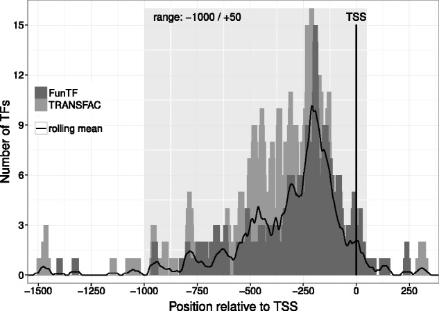
Choosing the promoter range. The great majority of the genuine fungal TFBS from TRANSFAC and FunTF map to the region −1000/+50 bp

2.5 CASSIS tool for SM cluster predictions

CASSIS is the successor of MDM published in 2013 (Wolf et al., 2013). It underwent several changes in the algorithm but the main idea remained the same: the sites for a TF regulating co-expressed cluster genes must be more dense (or form ‘islands’) within the cluster region.

CASSIS requires two input files: (i) genome sequence (contigs, chromosomes) in FASTA format; (ii) the corresponding annotation with start position, stop position and strand orientation of each gene. The user also needs a list of genes serving as ‘anchors’ for the future clusters. The latter can be SMIPS output or any other list of genes (e.g. manually selected). Principally, CASSIS is not restricted to only SM cluster predictions and will work for any anchor gene.

2.5.1 Promoter sequences

Before starting any prediction, CASSIS retrieves all promoter sequences genome-wide (based on the annotation file). The standard promoter range (−1000/+50 around TSS) applies if the intergenic region is >1 kb (or 2 kb for two non-overlapping promoters). If the promoter is bidirectional (overlapping) or the intergenic region is <1 kb, the whole intergenic region is retrieved. No promoter sequences are considered for genes overlapping by the 5′-ends.

2.5.2 Motif search

The tools MEME and FIMO (Bailey and Elkan, 1994; Grant et al. 2011; Bailey et al. 2009 (suite); http://www.meme-suite.org), required for the next two steps, are not incorporated into CASSIS and should be therefore pre-installed on the system.

The first three steps of the prediction (selection of the interim promoter sets, MEME and FIMO searches) are made as described in the initial MDM publication (Wolf et al., 2013). In short, motifs (putative binding sites) are searched in interim sets of promoters around the anchor gene. Since the length of the cluster and the location of the anchor gene within the cluster are unknown, CASSIS automatically prepares several promoter sets around the anchor ranging from three to 15 promoters upstream and downstream the anchor gene, in total up to 250 different sets (Fig. 2). All sets are sent to MEME for prediction of over-represented motifs.

Fig. 2.

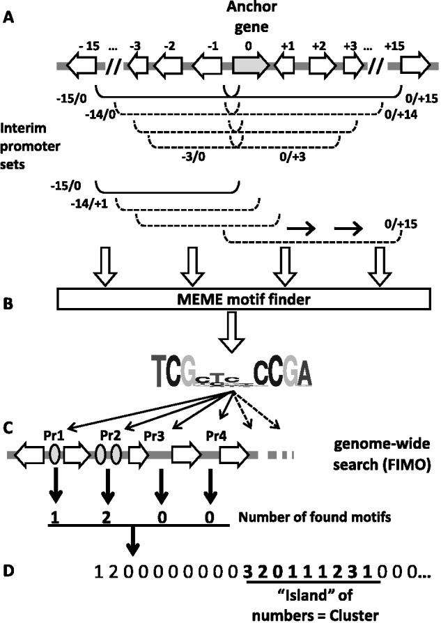
CASSIS algorithm. (A) Interim promoter sets around the anchor gene are submitted to MEME for motif prediction. (B) All found motifs are selected. (C) The motifs are submitted to FIMO for the genome-wide prediction in promoter (Pr) sequences. (D) The sequence of promoters, each characterized by the number of found motifs, is considered as the string of numbers. This number string is searched for an ‘island’ of mostly non-zero values, which is regarded as the cluster

MEME is run for each set with the following search parameters: any number of repetitions (ANR); one motif to find; motif width 6–12 bp. To select the motifs for further analysis, CASSIS applies the following restrictions: (i) the motif must be found in the promoter of the anchor gene; (ii) the motif must be in more than one promoter; and (iii) the MEME E-value must not exceed a certain estimated cut-off (see Section 2.5.5). All MEME input and output files are preserved.

The motifs fulfilling the requirements are automatically sent to FIMO (Grant et al., 2011), which predicts the motifs’ occurrences in all promoters of the considered genome. Thus, the FIMO input is the FASTA file with genome-wide extracted promoter sequences. The search is restricted by a p-value cut-off (see Section 2.5.5). Based on the FIMO results, CASSIS counts the number of motifs per promoter. At this step, the motif can be rejected if: (i) it is not found in the promoter of the anchor gene (this can happen because of the FIMO cut-off); (ii) it is not found in any other but the anchor promoter; (iii) the motif is too frequent, i.e. is found in more than a certain percentage of all promoter sequences (see Section 2.5.5 for parameter settings).

2.5.3 Transforming the genomic sequence into the sequence of promoters

On this step, the genomic sequence is seen as a sequence of promoters. This means that promoters are considered as units characterized by the number of occurrences of the considered motif (Fig. 2, Step D). The genomic sequence is in this way transformed into a string of numbers, each number representing the motifs’ occurrences in a unit (promoter). For instance, if one motif was found in the first promoter, two motifs in the second, and 0 in the third and fourth promoters, the string will be 1–2–0–0. SM clusters should represent the regions with the highest density of the motifs (in other words, ‘islands’ of non-zero numbers in the number string).

2.5.4 Defining the cluster borders

The anchor gene’s promoter is taken as seed for the cluster prediction. CASSIS scans the number string immediately upstream and downstream of the anchor promoter until it hits the first ‘zero’ value (promoter without binding site). If one or two zeroes are followed by a non-zero value, they are included in the cluster (gap rule ‘≤2 zero-promoters’, see Section 2.5.5). If more than two zeroes are found in a row, the cluster is interrupted. The last non-gap promoter marks the border of the cluster prediction. This step is carried out for each motif (Section 2.5.2). If this leads to multiple different cluster borders, the most abundant one will be considered. The output of CASSIS contains the locus IDs of the first and last genes corresponding to the promoters flanking the predicted cluster, the motif and promoter information, and the length of each prediction.

2.5.5 Adjustable parameters and their estimation

CASSIS can be fine tuned by adjusting four parameters, two of them being intrinsic CASSIS features, whereas the other two are the parameters of MEME and FIMO search. Since the motif prediction plays pivotal role in the further analysis, refining the latter by adjusting the E-value and p-value cut-offs for MEME and FIMO, respectively, can be crucial for the whole cluster prediction. The CASSIS default parameters for MEME and FIMO are estimated using the training set of experimentally verified SM clusters (Section 2.1). The option to tune these parameters is provided in CASSIS.

The two intrinsic CASSIS parameters are (i) the proportion of promoters with the motif in the genome (reflecting the genome-wide motif frequency); and (ii) the maximal allowed number of ‘zero’ promoters (‘gaps’) within the cluster. These parameters are estimated using a training set (e.g. of experimentally verified SM clusters) and can be further adjusted by the user. The gap parameter is restricted at the upper border by five promoters. The parameters are considered optimal if they give rise to the predictions with the smallest deviation. For the Ascomycete training set (Section 2.1), the parameter values were: frequency 14% and gap ≤2 zero-promoters (based on the observation of the largest gap in real clusters).

2.5.6 Runtime analysis

We applied CASSIS to the training set of 38 known gene clusters (Supplementary Table S1) on a machine with Intel Xeon CPUs running at 2.7 GHz. Using more than one CPU automatically turns on the parallelization of the MEME and FIMO steps. First, we allowed CASSIS to use up to 60 CPUs. Time measurements yield that it takes about 3 min in average to predict the cluster for a given anchor gene. Allowing only two CPUs, which should give results similar to a usual desktop computer, the prediction takes about 40 min in average.

3 Results

3.1 New features of CASSIS and prediction of SM enzymes by SMIPS

CASSIS is the improvement of the previously established MDM tool (Wolf et al., 2013). CASSIS is not similarity based and exploits the properties used for the definition of clusters, namely the co-localization and presumable co-regulation of cluster genes. The co-regulation assumes the occurrence of binding sites for the common regulator (TF) in the promoters of cluster genes. The task of the cluster prediction is thus restricted to the task of finding a region around the anchor gene, where the promoters share a common binding site. Importantly, the promoters sharing the site should form an ‘island’—a mostly uninterrupted group separated from non-cluster regions by long stretches of ‘motif-less’ promoters. This does not mean that the same sites cannot occur outside the cluster: they can exist but should be far enough not to interfere with the cluster (moreover, they can be indicators of other genes regulated by the same TF, thus the information about them can be valuable).

In the course of improvement of the MDM method and collecting more observations of real clusters, we realized that the prediction algorithm can be simplified, so that the scoring system applied in the MDM version can be dropped. Instead of the ‘frame scores’ used in MDM, we now applied a more straightforward approach of ‘gap rules’ as described in Section 2.5.4. This made the algorithm more transparent, easier to adjust and easier to interpret. Besides this innovation, we added and improved several features. We drastically increased the number of promoter sets (from 7 to 250), which are submitted to MEME for motif prediction. This makes the search for the best common motif more precise, improving the accuracy of the entire cluster prediction. We also introduced several cut-off values to filter out unpromising or invalid intermediate results: (i) the E-value cut-off for motifs predicted by MEME, (ii) the p-value cut-off for FIMO hits, (iii) the percentage cut-off for the number of promoters with binding sites compared with all promoters in the genome (genome-wide frequency of the motif), and (iv) the maximal gap length within the cluster. Altogether this helped to decrease the number of FP and to increase the specificity and accuracy (see Section 3.2).

To make the workflow smooth and independent, we added a small but useful tool called SMIPS for the preliminary prediction of (all potential SM anchor genes in the given genome.) Methodologically, SMIPS does not differ from other tools for PKS and NRPS predictions, basing on the HMM models for typical domains of SM enzymes. However, as CASSIS requires predefined anchor genes as input, we found it more convenient to add SMIPS to the CASSIS workflow. In this way, we avoid preliminary runs of other tools (such as SMURF) to obtain the anchor genes information. In addition to sending the output of SMIPS to CASSIS, it can be used independently for the annotation and description of SM genes.

3.2 Assessment of the CASSIS performance, validation and comparison with other tools

To assess the performance of our method and tool, we undertook a series of leave-one-out (LOO) cross-validation experiments. As positive set we used the 38 experimentally proven fungal clusters (Supplementary Table S1) and performed the LOO for each cluster. The benchmarking shows high specificity, sensitivity, accuracy and precision (Table 1). With this we show that over-fitting is not an issue and our tool is able to reliably predict unknown clusters.

Table 1.

Benchmark results of the LOO cross-validation for CASSIS

Characteristics	CASSIS performancea
Sensitivity	0.84 ± 0.0010
Specificity	0.98 ± 0.0002
Precision	0.71 ± 0.0010
Accuracy	0.96 ± 0.0002
FDR	0.29 ± 0.0010
F1-score	0.73 ± 0.0008

^aAverage for all 38 LOO experiments. Error is the standard error of the mean. See Supplementary Table S1 for the list of used clusters

As the CASSIS approach is based on promoter analysis and is thus very distant from similarity-based methods, it was interesting to compare its performance with the most prominent similarity-based tools antiSMASH and SMURF. We applied the tools to the re-identification of the clusters with known borders. To make a clean experiment and put all three tools in equal position, we included in our training set those clusters that were characterized before the publication of antiSMASH and SMURF and hence could be used for their training (at least for SMURF). On the other hand, the clusters published after 2010 were considered as ‘new’ for all three tools and used as test set. The comparison reveals that antiSMASH has a higher sensitivity but the number of FP predictions made by similarity-based methods is also higher: compared with CASSIS, antiSMASH suggests in average four FP more per cluster. This reflects the tendency of the similarity tools to overestimate the clusters’ lengths, even though they pick up the right genes with high sensitivity. As a result, CASSIS outperforms the other tools in specificity, accuracy and precision (Table 2, Supplementary Table S3 and Supplementary Fig. S1). Moreover, in some cases the similarity-based tools failed to recognize the anchor gene, which lead to the loss of the whole cluster (see Supplementary Fig. S2). For instance, in Aspergillus nidulans the ent-pimara-8(14),15-diene cluster is lost by antiSMASH and SMURF because they do not recognize AN1594 as the anchor gene. CASSIS/SMIPS did not encounter any problems in the detection of all anchors.

Table 2.

Comparison of CASSIS with the similarity-based antiSMASH and SMURF tools: re-identification of the 12 test clusters not used for the tools’ training

Characteristics	Comparisona
	CASSIS	antiSMASH	SMURF
Sensitivity	0.87 ± 0.04	0.94 ± 0.04	0.78 ± 0.10
Specificity	0.96 ± 0.01	0.87 ± 0.02	0.84 ± 0.02
Precision	0.80 ± 0.05	0.54 ± 0.05	0.42 ± 0.06
Accuracy	0.94 ± 0.01	0.88 ± 0.01	0.82 ± 0.02
FDR	0.20 ± 0.05	0.46 ± 0.05	0.58 ± 0.06
F1-score	0.81 ± 0.02	0.66 ± 0.04	0.51 ± 0.06

^aAverage for all 12 clusters. Error is the standard error of the mean. See Supplementary Table S1 for the list of used clusters

See Supplementary Table S4 for a more general comparison of the features of all four tools.

4 Discussion

Clustering of genes implies their co-localization, co-regulation and assignment to the same process. In the case of SM, this is a biosynthetic pathway and/or further processing of the product. Most of the approaches developed for the genome-wide cluster prediction rely on protein domain similarity. Thus, they use the first and last properties of the clusters but ignore the co-expression (or co-regulation). Our approach is in this sense complementary, as it ignores the functional features of the proteins but considers the promoter information. This constitutes both an advantage and a disadvantage of the approach. The advantage is the consideration of a new, yet unused layer of information (promoters, motifs, sites), which is, moreover, the key feature of the cluster definition. The disadvantage is the neglect of the remaining information, but this can be seen as a specialization. Indeed, the similarity-based tools exist and at least one of them, antiSMASH, gives very good, although not perfect, predictions. Our aim is not to compete with antiSMASH or to substitute it. We suppose that the optimal predictions can be achieved by application of both tools simultaneously: antiSMASH is more sensitive but CASSIS is more precise, and each of them supplies with specific information about the discovered clusters (see Supplementary Table S4).

Motifs that are shared by the cluster genes (and form in this way the basis of the cluster prediction) have their own value as the potential TFBS of the cluster’s presumable regulator. CASSIS provides the option to retrieve the motifs corresponding to the detected clusters. Moreover, as the motifs’ occurrences are scanned genome-wide, it is possible to find sub-clusters (also called super-clusters), which are groups of genes regulated by the same TF, simultaneously with the ‘main’ cluster, but located in another part of the genome. If a sub-cluster is large enough (more than three genes), it can be detected quite easily. In the next versions of CASSIS we plan to implement such a feature.

Like MDM, CASSIS is not restricted to the prediction of SM clusters. Other types of gene clusters can be represented by different anchor genes, depending on the pathway or process, for which the genes are clustered. As CASSIS does not consider the properties of genes, the nature of the anchor gene does not matter.

Being based on the de novo motif discovery, CASSIS is quite sensitive to the quality of the genome assembly. Two features are important: the length of contigs (scaffolds) and the information quality of the sequence. The former feature is, actually, important for any cluster prediction tool, since clusters are lengthy stretches of genomic sequence, which should be preferably uninterrupted. The information quality becomes important for genomes with low complexity (AT-rich) regions, since it is hard to predict significant motifs in such sequences.

5 Implementation and availability

The CASSIS method is implemented in a tool with the same name. User-friendly online versions of both SMIPS and CASSIS (the ‘CASSIS suite’) are available at https://sbi.hki-jena.de/cassis. The suite also provides a comfortable workflow to run CASSIS on the results of SMIPS. The source codes as well as executeable files for Linux and Windows are freely available at https://sbi.hki-jena.de/cassis/Download.php. The SMIPS and CASSIS tools are implemented in Perl 5.

References

- Amaike S., Keller N.P. (2011) Aspergillus flavus In: VanAlfen N., et al. (ed.) Annual Review of Phytopathology. Vol. 49, pp. 107–133. [DOI] [PubMed] [Google Scholar]
- Andersen M.R. et al. (2013) Accurate prediction of secondary metabolite gene clusters in filamentous fungi. Proc. Natl Acad. Sci., 110, E99–E107. [DOI] [PMC free article] [PubMed] [Google Scholar]
- Bailey T.L., Elkan C. (1994) Fitting a mixture model by expectation maximization to discover motifs in biopolymers. In Proceedings/International Conference on Intelligent Systems for Molecular Biology; ISMB, Vol. 2, AAAI Press, pp. 28–36. [PubMed]
- Bailey T.L. et al. (2009) MEME Suite: tools for motif discovery and searching. Nucleic Acids Res., 37, W202–W208. [DOI] [PMC free article] [PubMed] [Google Scholar]
- Bergmann S. et al. (2010) Activation of a silent fungal polyketide biosynthesis pathway through regulatory cross talk with a cryptic nonribosomal peptide synthetase gene cluster. Appl. Environ. Microbiol., 76, 8143–8149. [DOI] [PMC free article] [PubMed] [Google Scholar]
- Blin K. et al. (2013) antiSMASH 2.0—a versatile platform for genome mining of secondary metabolite producers. Nucleic Acids Res., 41, W204–W212. [DOI] [PMC free article] [PubMed] [Google Scholar]
- Boettger D. et al. (2012) Evolutionary imprint of catalytic domains in fungal PKS-NRPS hybrids. ChemBioChem, 13, 2363–2373. [DOI] [PubMed] [Google Scholar]
- Brakhage A.A. (2013) Regulation of fungal secondary metabolism. Nat. Rev. Microbiol., 11, 21–32. [DOI] [PubMed] [Google Scholar]
- Brakhage A.A., Schroeckh V. (2011) Fungal secondary metabolites—strategies to activate silent gene clusters. Fungal Genet. Biol., 48, 15–22. [DOI] [PubMed] [Google Scholar]
- Cerqueira G.C. et al. (2014) The Aspergillus Genome Database: multispecies curation and incorporation of RNA-Seq data to improve structural gene annotations. Nucleic Acids Res., 42, D705–D710. [DOI] [PMC free article] [PubMed] [Google Scholar]
- Do J., Miyano S. (2008) The GC and window-averaged DNA curvature profile of secondary metabolite gene cluster in Aspergillus fumigatusy genome. Appl. Microbiol. Biotechnol., 80, 841–847. [DOI] [PubMed] [Google Scholar]
- Eppelmann K. et al. (2002) Exploitation of the selectivity-conferring code of nonribosomal peptide synthetases for the rational design of novel peptide antibiotics. Biochemistry, 41, 9718–9726. [DOI] [PubMed] [Google Scholar]
- Grant C.E. et al. (2011) FIMO: scanning for occurrences of a given motif. Bioinformatics, 27, 1017–1018. [DOI] [PMC free article] [PubMed] [Google Scholar]
- Hoffmeister D., Keller N.P. (2007) Natural products of filamentous fungi: enzymes, genes, and their regulation. Nat. Prod. Rep., 24, 393–416. [DOI] [PubMed] [Google Scholar]
- Keller N.P., Hohn T.M. (1997) Metabolic pathway gene clusters in filamentous fungi. Fungal Genet. Biol.: FG & B, 21, 17–29. [PubMed] [Google Scholar]
- Khaldi N. et al. (2010) SMURF: genomic mapping of fungal secondary metabolite clusters. Fungal Genet. Biol., 47, 736–741. [DOI] [PMC free article] [PubMed] [Google Scholar]
- Stachelhaus T. et al. (1999) The specificity-conferring code of adenylation domains in nonribosomal peptide synthetases. Chem. Biol., 6, 493–505. [DOI] [PubMed] [Google Scholar]
- Starcevic A. et al. (2008) ClustScan: an integrated program package for the semi-automatic annotation of modular biosynthetic gene clusters and in silico prediction of novel chemical structures. Nucleic Acids Res., 36, 6882–6892. [DOI] [PMC free article] [PubMed] [Google Scholar]
- Weber T. et al. (2009) CLUSEAN: a computer-based framework for the automated analysis of bacterial secondary metabolite biosynthetic gene clusters. J. Biotechnol., 140, 13–17. [DOI] [PubMed] [Google Scholar]
- Wolf T. et al. (2013) Motif-based method for the genome-wide prediction of eukaryotic gene clusters In: Petrosino A., et al. (eds), New Trends in Image Analysis and Processing – ICIAP 2013, Number 8158 in Lecture Notes in Computer Science, Springer, Heidelberg, pp. 389–398. [Google Scholar]
Associated Data
This section collects any data citations, data availability statements, or supplementary materials included in this article.