Mesochronal Structure Learning

Abstract

Standard time series structure learning algorithms assume that the measurement timescale is approximately the same as the timescale of the underlying (causal) system. In many scientific contexts, however, this assumption is violated: the measurement timescale can be substantially slower than the system timescale (so intermediate time series datapoints will be missing). This assumption violation can lead to significant learning errors. In this paper, we provide a novel learning algorithm to extract system-timescale structure from measurement data that undersample the underlying system. We employ multiple algorithmic optimizations that exploit the problem structure in order to achieve computational tractability. The resulting algorithm is highly reliable at extracting system-timescale structure from undersampled data.

1 Introduction

In many domains, measurement speed can be significantly slower than the causal or communication speeds in the underlying system. For example, fMRI experiments typically measure brain activity roughly every two seconds, but the causal and communication connections between neuronal layers operate much faster [8]. Similar observations can be made about systems in ecology, climatology, economics, genomics and proteomics, and cognitive science. Moreover, a discrepancy between the measurement timescale τ_M and the system timescale τ_S can make a difference: an apparent A → B connection at τ_M can be consistent with any possible connection at τ_S: A → B, A ← B, or no connection at all. Thus, it is critical that we not simply restrict our attention to learning connections at τ_M.

In this paper, we address the problem of learning the causal structure at τ_S from measurements taken at a slower sampling rate, also called “undersampled” data.¹ We focus on cases in which the underlying system structure can be represented as a directed graphical model (without simultaneous influence). There has been very little prior work on the problem of structure learning from undersampled time series data, though there have been important prior explorations of learning when the measurement and system timescales diverge, or when causal influences operate on multiple timescales [3, 5, 9]. There are multiple algorithms for learning graphical structure from time series data [6, 7, 11, 14, 15], but they all assume that τ_M is at least as fast as τ_S. Undersampling was explicitly addressed in [2], but they focused on the “forward” problem of undersampling: given a structure at τ_S, what structure will be realized at τ_M? That paper provided some preliminary theorems (used below) to characterize the backward problem, but not a usable algorithm for actually learning structure at τ_S from measurements at τ_M. In this paper, we introduce such an algorithm: the Mesochronal Structure Learning (MSL) algorithm (from Greek méso (μέσω) for “through” and chronos (χρóνoς) for “time”) (Section 3); and show that it can often learn significant τ_S structure from τ_M data (Section 4). First, however, we provide a precise statement of the problem.

2 Formal statement of the problem

We use a compressed graph representation of the underlying system structure.² We assume that the system is first-order Markov,³ and so temporal information can be encoded directly in the graphical edges. This assumption also implies a form of “causal sufficiency”: specifically, there cannot be unobserved variables such that nodes in the current timestep (at the causal timescale) are conditionally associated once the variable values at the previous timestep are known. Let $\mathcal{G}$ be a directed graphical model over variables V such that V_i → V_j means $V_i^{t-1}\to V_j^t$, where superscripts denote (relative) time index. We exclude contemporaneous connections because τ_S can be arbitrarily fast. $\mathcal{G}$ can be cyclic, including self-loops, but the underlying system structure will be acyclic when “unrolled” through time. Let P (2V) be a joint probability distribution over V^t and V^t−1. We connect $\mathcal{G}$ and P (2V) through standard assumptions, though adjusted for this setting. Specifically, let pa(V_i) denote the parents of V_i in $\mathcal{G}$. The Markov assumption requires: $V_i^t$ is independent of $\left[{\mathbf{V}}^t\backslash V_i^t\right]\cup \left[{\mathbf{V}}^{t-1}\backslash \text{pa}{\left(V_i\right)}^{t-1}\right]$ conditional on $\text{pa}{\left(V_i\right)}^{t-1}$. The Faithfulness assumption requires that these be the only independencies involving some $V_i^t$.

Let {t⁰, t¹, …, t^k, …} denote the timesteps at the system timescale. We say that the system is sampled at rate u when the measured timesteps are {t⁰, t^u, …, t^ku, … }. The system timescale is thus “sampled at rate 1.” We focus on cases of undersampling; that is, when u > 1. Undersampling implies failure to observe intermediate steps on paths between variables, and so the measurement timescale graph ${\mathcal{G}}^u$ can be derived from the causal timescale graph ${\mathcal{G}}^1$. More precisely, V_i → V_j in ${\mathcal{G}}^u$ iff there is a path of length u from V_i to V_j in ${\mathcal{G}}^1$. Undersampling can also introduce bidirected edges that represent unobserved common causes of variables at time t. For example, if V_i ← V_c → V_j in ${\mathcal{G}}^1$, then for all u > 1, ${\mathcal{G}}^u$ will contain V_i ↔ V_j since the unmeasured $V_c^{t-1}$ is a parent of both $V_i^t$ and $V_j^t$. If the true system structure ${\mathcal{G}}^1$ and the sampling rate u are known, then there are efficient algorithms for computing the resulting (expected) measurement timescale structure ${\mathcal{G}}^u$ [2].

The general problem of inferring ${\mathcal{G}}^1$ from data sampled at unknown rate u is computationally intractable at the current time, and so we principally focus on the special case in which u = 2 (though Section 4 shows how to generalize our algorithm to u > 2). That is, what can be learned about ${\mathcal{G}}^1$ if the input data is a time series in which every other timestep is unobserved? It is straightforward to see that ${\mathcal{G}}^2$ can be quite different from ${\mathcal{G}}^1$; for example, if ${\mathcal{G}}^1$ is a directed cycle over three variables (e.g., X → Y → Z → X), then that cycle will have the reverse direction in ${\mathcal{G}}^2$. At the same time, ${\mathcal{G}}^2$ and ${\mathcal{G}}^1$ cannot be arbitrarily different; for example, if V_i → V_i in ${\mathcal{G}}^1$ (i.e., V_i has a self-loop), then V_i → V_i in ${\mathcal{G}}^2$. We now provide a multi-step algorithm for recovering as much information as possible.

3 MSL algorithm

There are a number of previously identified structural invariants of ${\mathcal{G}}^1$ that hold across sampling rates [2], but many of them provide only a coarse characterization of the structure of ${\mathcal{G}}^1$. We thus must search in a more direct fashion for the ${\mathcal{G}}^1$ that could have produced ${\mathcal{G}}^2$. The Mesochronal Structure Learning (MSL) algorithm has two distinct steps. First, one learns ${\mathcal{G}}^2$ from data, expert knowledge, or a combination of the two (Section 3.1). There are many different algorithms for learning causal structure at the measurement timescale (i.e., ${\mathcal{G}}^2$), and so we focus on the second step: infer the set of ${\mathcal{G}}^1$ that could possibly have produced (given undersampling) the learned ${\mathcal{G}}^2$ (Section 3.2). The ${\mathcal{G}}^2\to {\mathcal{G}}^1$ mapping is one-to-many, and so the MSL algorithm out-puts an equivalence class (possibly a singleton) of possible ${\mathcal{G}}^1$. The MSL algorithm is based on a conceptually simple inferential move, but requires significant algorithmic (Section 3.3) and practical (Section 3.4) optimizations in order to be computationally tractable.

3.1 Learning ${\mathcal{G}}^2$

There are many different algorithms for learning the structure of ${\mathcal{G}}^2$ from time series data [6, 7, 11, 14, 15], as the measurement and structure timescales are the same. One can also modify structure learning algorithms designed for i.i.d. data (e.g., the well-known PC or GES algorithms [1, 13]) for the special case of time series data in which the causal direction can be inferred from temporal information. We will mostly treat these algorithms as “black boxes” that simply provide an estimated ${\mathcal{G}}^2$ for input to the second stage. We cannot completely abstract away from details of those algorithms, however, since errors learning ${\mathcal{G}}^2$ structure can result in errors by the overall MSL algorithm. We return to this issue in Section 4, but focus for now on the algorithmically novel aspect of inferring causal timescale structure from estimated measurement timescale structure.

3.2 From ${\mathcal{G}}^2$ to ${\mathcal{G}}^1$

Given a known ${\mathcal{G}}^1$ and undersample rate u, [2] provides an efficient method for computing ${\mathcal{G}}^u$. Thus, for an estimated ℋ², there is an obvious brute-force approach: for all ${\mathcal{G}}^1$, compute the corresponding ${\mathcal{G}}^2$ and check if it equals the estimated ℋ². The problem with this approach is equally obvious: it must survey every possible ${\mathcal{G}}^1$, of which there are $2^{n^2}$ many. This brute-force strategy could potentially work for 3-, 4-, or even 5-node graphs, but rapidly becomes computationally completely infeasible. We thus pursue a different strategy.

We focus throughout on the case of a single Strongly Connected Component (SCC): a maximal variable set S such that there is a path from every X ∈ S to every Y ∈ S. All systems with feedback are composed of SCCs, and so they are the most scientifically interesting systems when working with time series data. When a very weak additional condition holds,⁴ then SCC membership is invariant under undersampling (Corollary 7 in [2]). Thus, we can use ${\mathcal{G}}^2$ structure to reliably identify SCC membership in ${\mathcal{G}}^1$, and then do focused search over each SCC separately.

Theorems 4 and 5 in [2] show that, when u gets very large, such an SCC becomes a super-clique: for every pair of nodes A, B (possibly A = B), we have A → B, A → B, and A ↔ B. (The last two do not apply when A = B.) That is, a super-clique is a maximally dense graph over the SCC. Moreover, these super-cliques are the worst-case for a “backwards” learning algorithm, as a huge number of SCCs imply a super-clique under (significant) undersampling. Thankfully, super-cliques rarely result for smaller undersample rates; typically, more can be learned at u = 2.

Given an estimated ℋ² that is an SCC, every directed edge corresponds to a path of length 2 in ${\mathcal{G}}^1$. More generally, if we have estimated ℋ^u for a known u, then each edge must correspond to a path of length u in ${\mathcal{G}}^1$. Thus, we can add u − 1 “virtual” nodes within each edge in ℋ^u, where each virtual node refers to some unknown, but actual, node in V. The virtual-to-actual node mapping can clearly be many-to-one, as u can be significantly larger than the size of V. This virtual node representation is shown in Figure 1.

Figure 1.

A 3-node SCC at undersampling rates 1 and 2, as well as its virtual nodes and their merging options.

The basic structure of this stage of the MSL algorithm is: (1) “identify” each virtual node with an actual node, thereby yielding a candidate ${\mathcal{G}}^1$; and then (2) check if that candidate actually implies ℋ^u. As noted above, there is a computationally efficient algorithm for step (2); the computational challenge is efficiently considering the relevant possible identifications. We focus in the remainder of this section on the case of u = 2 as that is sufficient to reveal significant complexities. The overall algorithm-schema is importantly not limited to that case, however, and we provide a “proof-of-concept” for u = 3 in Section 4.

For e edges in ℋ², there are n^e possible node identifications,⁵ each of which results in a candidate ${\mathcal{G}}^1$. Moving directly to complete identifications can require examining an intractable number of ${\mathcal{G}}^1$ (e.g., if n > 30 and e > 100, as below). We thus instead sequentially identify virtual nodes, coupled with a (local) stopping rule based on the concept of a conflict, and a lemma (with corollary):⁶

conflict

${\mathcal{G}}^u$ contains one or more edges that are not in ℋ^u.

Lemma 3.1. Conflict persistence

If a virtual node identification results in a conflict, then no further node identifications will eliminate that conflict.

Corollary 3.2

If ${\mathcal{G}}^1$ conflicts with ℋ^u, then every supergraph of ${\mathcal{G}}^1$ conflicts with ℋ^u.

Thus, if any partial virtual node identification results in a ${\mathcal{G}}^1$ whose ${\mathcal{G}}^u$ contains an edge not found in ℋ^u, then we need not consider any further identifications that build off of that base. This naturally suggests a backtracking search on a search tree through the possible node identifications, as shown in Figure 2. More precisely, the basic MSL algorithm is:

1. Let $\mathcal{G}$ be the empty graph, and {E₁, …, E_e} be an arbitrary ordering of edges in ℋ^u (Table in Figure 1)

2. In a depth-first manner over the edges, consider each possible node identification for the virtual nodes added to E_i and add the corresponding edges to $\mathcal{G}$

3. Check whether a conflict is found after adding the edges arising from virtual node identification for E_i

4. If a conflict is found, then prune that search tree branch, backtrack by removing the E_i identification, and try the next possible node identifications for E_i.

Figure 2.

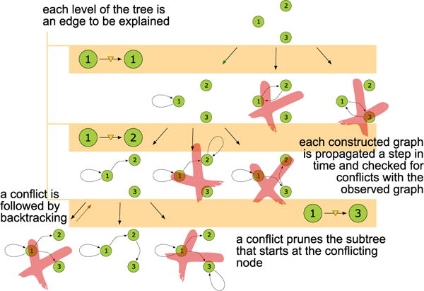
The search tree for 3-node SCC of Figure 1

The process is illustrated in Figure 2 for the graph in Figure 1. In the worst case, this algorithm obviously requires checking as many ${\mathcal{G}}^1$ as if we simply surveyed all possible simultaneous node identifications. In practice, however, the proactive pruning of branches in the search tree can lead to considerable speed-ups, especially in cases in which e is relatively large.

This algorithm is correct but not yet complete, as ${\mathcal{G}}^1$ can contain edges that do not have manifest in any way in ${\mathcal{G}}^2$. For example, if ${\mathcal{G}}^1$ is A → B, then ${\mathcal{G}}^2$ is simply the empty graph over A, B. In that case, there are no virtual nodes to identify, so the algorithm would correctly but incompletely return the empty graph as the only ${\mathcal{G}}^1$ possibility. More generally, especially for relatively dense ℋ², the algorithm finds a suitable ${\mathcal{G}}^1$ prior to reaching the full depth of the search tree (i.e., without identifying all virtual nodes). One response would be to simply force the algorithm to fully traverse the tree, but this can be quite expensive when the branching factor is high (i.e., for dense ℋ²). Instead, we pursue a different strategy.

If the algorithm finds a suitable ${\mathcal{G}}^1$ before reaching a leaf of the search tree, then we know that every graph below it in the tree will be a supergraph of that ${\mathcal{G}}^1$ (since virtual node identifications can only add edges, not remove them). Thus, we only need to find all supergraphs of that ${\mathcal{G}}^1$ whose ${\mathcal{G}}^2={\mathcal{H}}^2$. That search is greatly aided by Corollary 3.2.

The supergraph construction step first tries to separately add each of the n² possible directed edges that are not yet in ${\mathcal{G}}^1$. Each resulting graph that equals ℋ² is added to the output equivalence class. The step then adds, in a depth-first manner, each edge that did not yield a conflict to the other new graphs, and backtracks whenever an edge addition creates a conflict.⁷ This step is extremely fast in practice for graphs of reasonable sparsity despite its worst-case factorial behavior. If no edges create a conflict—for example, when ℋ² is a super-clique—then the running time is indeed Θ(n!). In that particular case, however, the equivalence class has been analytically determined to be any size-n SCC with gcd=1 (see ^{fn. 4}) [2, Theorem 4], and so the present algorithm is actually unnecessary.

The full MSL algorithm (including the supergraph step) has the following desirable property:

Lemma 3.3

The MSL algorithm is correct and complete: given ℋ², it finds all and only ${\mathcal{G}}^1$ such that ${\mathcal{G}}^2={\mathcal{H}}^2$.

Unfortunately, preliminary experiments demonstrated that the algorithm can be very slow (see Figure 4 for a highlight of the problem) and take days even for smaller (n = 10) graphs. The order in which virtual nodes are identified can make a significant difference in runtime speed, but even improving those orders is insufficient to yield an algorithm that is usable on large graphs. Instead, we must exploit additional constraints and optimizations.

Figure 4.

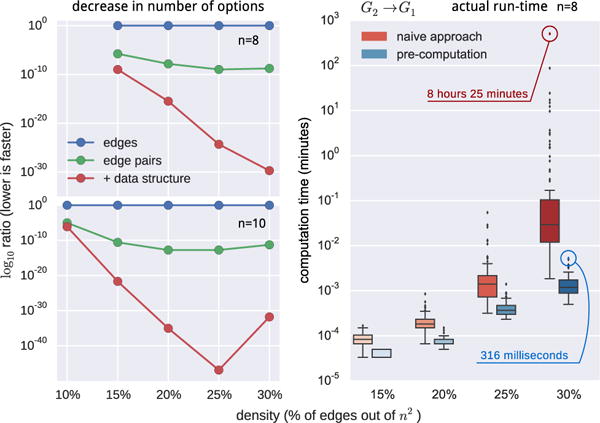
Comparison of the search-space size (left) and computation time (right) between the naive backtracking and our approaches.

3.3 Using graphical constraints

The key intuition underlying the constraints in this section is that some virtual node identifications can be excluded without ever actually constructing-and-testing the corresponding ${\mathcal{G}}^1$. For example, suppose A → B → C in ℋ². In this case, ${\mathcal{G}}^1$ must contain, for some X, Y: A → X→ B → Y → C. There is thus a length-2 path from X to Y in ${\mathcal{G}}^1$, and so ${\mathcal{G}}^2$ will contain X → Y. Hence, we only need to consider virtual node identifications for A → B and B → C in which the two identifications correspond to nodes with a directed edge between them in ℋ². More generally, virtual node identifications can analytically constrain one another in ways that can be exploited in this algorithm.

Recall that the complexity of the MSL algorithm for u = 2 is approximately n^e, where e is the number of edges in ℋ². By identifying pairs of virtual nodes (that analytically constrain one another), we can potentially achieve a large reduction in the exponent in practice, since we will have to consider many fewer branches.

Two different types of structures in ℋ² guide the pairwise identifications. First, consider all forks in ℋ²: pairs of edges X ← H → Y, where possibly X = H or Y = H (if there is a self-loop plus another edge). If the two virtual nodes refer to the same actual node, then X and Y will have a common cause in the previous (causal) timestep, and so there will be a bidirected edge between them.⁸ Thus, if there is no bidirected edge between X and Y in ℋ², then the two virtual nodes cannot identify to the same node. Hence, we only need to consider n² − n possible identifications for that pair of virtual nodes.

The other relevant structure is the two-edge chain described at the start of this section, where the only pairwise virtual node identifications that are considered are those for which there is a corresponding edge in ℋ².

In practice, the algorithm converts some elements of the edge list {E₁, …, E_e} into edge-pairs by first selecting (without replacement)} all forks in ℋ², then selecting all remaining two-edge directed paths. The remaining edges have the usual n possible virtual node identifications.

Figure 3 shows a search space for the graph from Figure 1, and demonstrates the computational advantage of considering pairwise identifcations, as the number of possible identifications is significantly reduced.

Figure 3.

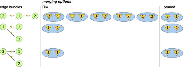
Edge-pairs for 3-node SCC of Figure 1 and merging options for their virtual nodes: all possible options (raw) and the one that remain after constructing the pairwise data structure (pruned).

In general, let {m₁, …, m_l} be the sets of virtual node identifications for each of the edges or edge-pairs derived from the preceding procedure. The computational complexity of using some edge-pairs is simply ${\prod }_i^l\text{len}\left(m_i\right)$, where len is the number of possible identifications for that particular edge or edge-pair. Thus, the computational advantage, expressed as a log-ratio, of using (some) edge-pairs is: $\log r={\displaystyle {\sum }_i^l\log \text{len}(m_i)-e\log n}$. This advantage is plotted in Figure 4, which shows (on log-scale) the average log-ratio for 100 random 8- and 10-node SCCs. The practical advantage of edge-pairs is potentially even greater, as Figure 4 does not account for active pruning of the search tree.

3.4 Precomputation and other optimizations

The use of edge-pairs provides significant speed-up in the MSL algorithm (as seen in Figure 4), but its worst-case complexity still makes it difficult to use the algorithm for n > 10. Moreover, around 10% of the graphs took many days to compute, and did not exhibit any noticeable structural difference in ℋ² that could be used to predict computation time.⁹ The core problem is that much of the search tree eventually gets pruned, but structural features of ℋ² do not support predictions about which parts will be pruned. If we can instead prune conflicting options prior to the traversal of the solution space, then we can potentially further reduce the search time.

The key algorithmic move is to expand the “analytic conflict checking” beyond just particular edge-pairs, to also pre-computing conflicts between multiple edge-pairs. In the extreme, there can be a (seemingly) possible virtual node identification that conflicts with every possible identification for some other edge or edge-pair, in which case the first identification can simply be removed from consideration. Moreover, this precomputation is independent of the evaluation order of the virtual node identifications, since a conflict between identifications m_i and m_j does not depend on the particular values i and j. This pruning thus also reduces the need for random restarts to be robust against evaluation order effects.

The MSL algorithm was therefore expanded to include significant pre-computation to further prune the initial search tree. Specifically, for each pair of edge-pairs, the algorithm constructs a ${\mathcal{G}}^1$ for every possible identification of both edge-pairs. If the resulting ${\mathcal{G}}^1$ results in a conflict with ℋ², then we remove that pair of complex identifications from the search tree. This precomputation can considerably prune the search tree, perhaps even yielding (as in Figure 3) a search “tree” with only one branch. There is a cost because the resulting data structure can be complex: it contains not only the reduced set of (complex) identifications for each edge-pair, but also splits those options into subsets depending on the particular (complex) identification used in the previous level of the search tree. This more complex structure is required because some possible identifications will be incompatible with only a subset of the identifications at the previous level, but we want to avoid checking them during the algorithm flow (since we already checked in the precomputation).

Further algorithmic speed-ups can be achieved by intelligently ordering the virtual node identifications (i.e., the levels of the search tree). In particular, the MSL algorithm will run fastest when search tree levels with significant breadth—that is, virtual nodes or node-pairs for which there are many possible identifications—are pushed further down in the search tree. If this is done, then pruning operations will remove more branches. In addition, each search tree node is also a “conflict check” point, and this ordering of search tree levels minimizes the number of search tree nodes, even if no branches are ever pruned. The benefits of intelligent identification ordering can be substantial for deep trees with small numbers of possible identifications for most of the edge-pairs.

These two optimizations—precomputation and intelligent search tree ordering—yield substantial benefits. We again computed the potential reduction in computation for randomly generated graphs (using the equation from Section 3.3). The “+ data structure” line on the left-hand plot in Figure 4 shows that the more optimized approach can achieve over 40 orders of magnitude reduction in the number of conflict checks.

Each conflict check requires the algorithm to add edges to the constructed ${\mathcal{G}}^1$, compute ${\mathcal{G}}^2$, check for conflicts with ℋ², and then remove the just-added edges in case of a conflict. These steps are computationally expensive, and so we can achieve further performance gains if we can analytically determine whether a complex identification creates a conflict before starting these operations. These checks are not precomputed, but rather are performed in an online fashion based on the constraints in the following lemmas (where $c{h}_{\mathcal{G}}\left(A\right)$ and $p{a}_{\mathcal{G}}\left(A\right)$ denote the children and parents of A in $\mathcal{G}$, respectively):

Lemma 3.4

A virtual node V in $S\stackrel{V}{\to }E$ cannot be identified with node X if any of the following holds:

1. $\exists W\in c{h}_{{\mathcal{G}}^1}\left(S\right)\backslash Xs.t.\cancel{\exists }W\leftrightarrow X\in {\mathcal{H}}^2$

2. $\exists W\in c{h}_{{\mathcal{G}}^1}\left(X\right)\backslash Es.t.\cancel{\exists }W\leftrightarrow E\in {\mathcal{H}}^2$

3. $\exists W\in c{h}_{{\mathcal{G}}^1}\left(X\right)s.t.\cancel{\exists }S\to W\in {\mathcal{H}}^2$

4. $\exists W\in c{h}_{{\mathcal{G}}^1}\left(E\right)s.t.\cancel{\exists }X\to W\in {\mathcal{H}}^2$

5. $\exists W\in p{a}_{{\mathcal{G}}^1}\left(S\right)s.t.\cancel{\exists }W\to X\in {\mathcal{H}}^2$

6. $\exists W\in p{a}_{{\mathcal{G}}^1}\left(X\right)s.t.\cancel{\exists }W\to E\in {\mathcal{H}}^2$

Lemma 3.5

A virtual node pair V₁, V₂ for a fork $E_1\stackrel{V_1}{\leftarrow }S\stackrel{V_2}{\to }{E}_2$ cannot be identified with nodes X₁, X₂ if any of the following holds:

1. $V_{1}in{E}_1\stackrel{V_1}{\leftarrow }S\mathit{\text{cannot be identified with}}{X}_1$

2. $V_{2}inS\stackrel{V_2}{\to }{E}_2\mathit{\text{cannot be identified with}}{X}_2$

3. $V_1\equiv E_2\wedge V_2\notin p{a}_{{\mathcal{H}}^2}\left(E_1\right)$

4. $V_2\equiv E_1\wedge V_1\notin p{a}_{{\mathcal{H}}^2}\left(E_2\right)$

5. $S\equiv V_2\wedge V_1\ne V_2\wedge V_1\ne E_2\mathit{\text{and}}\cancel{\exists }{E}_2\leftrightarrow V_1\in {\mathcal{H}}^2$

6. $S\equiv V_1\wedge \left(V_1\equiv V_2\vee V_2\equiv E_2\right)\mathit{\text{and}}\cancel{\exists }{E}_1\leftrightarrow E_1\leftrightarrow E_2\in {\mathcal{H}}^2$

7. $S\equiv V_1\wedge \left(V_1\equiv V_2\vee V_2\equiv E_2\right)\mathit{\text{and}}\cancel{\exists }{E}_1\leftrightarrow E_2\in {\mathcal{H}}^2$

8. $S\equiv V_2\wedge \left(V_1\equiv V_2\vee V_1\equiv E_1\right)\mathit{\text{and}}\cancel{\exists }{E}_1\leftrightarrow E_2\in {\mathcal{H}}^2$

9. $V_1\equiv V_2\mathit{\text{and}}\cancel{\exists }{E}_1\leftrightarrow E_2\in {\mathcal{H}}^2$

Lemma 3.6

A virtual node pair V₁, V₂ for two-edge sequence $S\stackrel{V_1}{\to }M\stackrel{V_2}{\to }E$ E cannot be identified with X₁, X₂ if any of the following holds:

1. $V_{1}inS\stackrel{V_1}{\to }M\mathit{\text{cannot be merged to}}{X}_1$

2. $V_{2}inM\stackrel{V_2}{\to }E\mathit{\text{cannot be merged to}}{X}_2$

3. $V_1\equiv V_2\wedge \left(M\notin p{a}_{{\mathcal{H}}^2}\left(M\right)\vee V_1\notin p{a}_{{\mathcal{H}}^2}\left(V_2\right)\vee S\notin p{a}_{{\mathcal{H}}^2}\left(E\right)\right)$

As noted above, we apply these constraints in an online manner in order to prune branches of the search tree without having to add edges and check for conflicts. The resulting algorithm exhibits substantial reductions in runtime, enabling us to examine the MSL algorithm’s behavior for ${\mathcal{G}}^1$ ranging up to 35 nodes, as shown in the simulation testing described in the next section.

4 Testing and validation

As we argued earlier, SCCs represent the scientifically most interesting situations, precisely because they are ones in which feedback loops present a challenging learning task. In addition, although connections between SCCs are undoubtedly of interest, the formal results of [2] imply that we can reliably treat the SCCs relatively independently. We thus focus on single-SCC graphs in our synthetic data studies. Any SCC can provably be decomposed into a single simple loop with “ears” (i.e., sequences that branch off from, then return to, that simple loop) that build on top of one another. We thus use a simple ear decomposition skeleton to generate SCCs for our simulations.

SCC generation procedure

For n nodes, first generate a single simple loop that passes through all nodes. Without loss of generality, we can assume that this ring graph passes through the nodes in sequential order. There are n(n − 1) possible edges that can be added to this ring graph, including self-loops for each node. We sample uniformly from those possible edges until the required density—i.e., the fraction of the n² possible edges that are actual—is achieved.¹⁰ We use overall density rather than average node degree to measure graph complexity because density is normalized by the number of possible edges, so we can (approximately) match graph complexity across different values of n.

We previously reported the theoretical maximum conflict checks for 8- and 10-node graphs for different versions of the MSL algorithm. We also report (in Figure 4) a comparison of the actual run times. We randomly generated 100 8-node graphs for each density in {15%, 20%, 25%, 30%} and ran both the naive approach (virtual node identification for each edge separately) and the precomputation approach that takes advantage of edge-pairs and pairwise constraints. The box and whisker plot shows the distribution of the individual run-times expressed in minutes. Not only does the median execution time for 8-node graphs improve by an order of magnitude, but the naive approach also generates considerably more outliers that take much longer to compute. The run-times for the hardest graphs (which provide an empirical estimate on the run-time upper bound) are five orders of magnitude longer for the naive approach.¹¹

4.1 Equivalence class sizes

We earlier noted that, when ℋ² is a super-clique (i.e., every possible edge between each pair of nodes), then there will typically be a large number of ${\mathcal{G}}^1$ consistent with that super-clique. That is, the equivalence class will be quite large. One question is about the sizes of the equivalence classes when ℋ² is not a super-clique. If the equivalence class is sufficiently small, then expert knowledge or further studies may be a tractable way to reach a unique solution.

To better explore the equivalence class sizes, we generated 100 random 6-node SCCs (using the above procedure) for each density from 20% to 60% in 5% increments, then analytically computed ${\mathcal{G}}^2$ and passed that to the optimized MSL algorithm. n = 6 is sufficiently large that brute-force inference is infeasible, but the graphs are still tractable for the optimized MSL algortihm even at high densities. This is a particular worry since the complexity of the search grows exponentially with the number of edges in ${\mathcal{G}}^2$. Figure 5 shows the sizes of the equivalence classes for the graphs at different densities.

Figure 5.

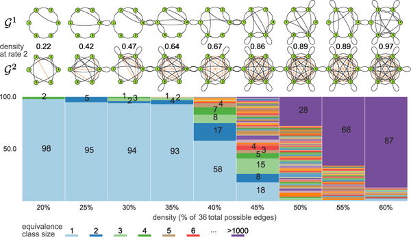
Equivalence class size distribution among 100 randomly generated 6-node SCCs at a given density and examples of 6-node SCCs for each.

Some of the most notable findings from Figure 5 are i) for densities up to 35%, the overwhelming majority of the equivalence classes are singletons; ii) for densities above 50%, the equivalence classes often grow to quite large sizes; however, iii) those ${\mathcal{G}}^2$ graphs are incredibly dense, and so unsurprisingly are difficult to analyze tractably. The MSL algorithm complexity depends exponentially on the number of edges in ${\mathcal{G}}^2$, and so increasing n for a fixed density rapidly leads to significant computational barriers. Figure 5 suggests that densities above 35% will frequently lead to very large equivalence classes, and so we focus on lower densities for larger n.

In particular, we performed the same analysis (including run-times) for 8-node (Figure 6) and 10-node graphs (Figure 7). The results for 6-node graphs largely generalize. MSL is a fast and practical algorithm for these graph sizes, as demonstrated by the wall-clock run-time measurements summarized in Figure 7. Note that these are quite challenging graphs, as shown in Figure 8. 10-node graphs with 30% density can have more than 65 edges in ${\mathcal{G}}^2$, and so the naive approach would have to consider 10⁶⁵ virtual node identifications.

Figure 6.

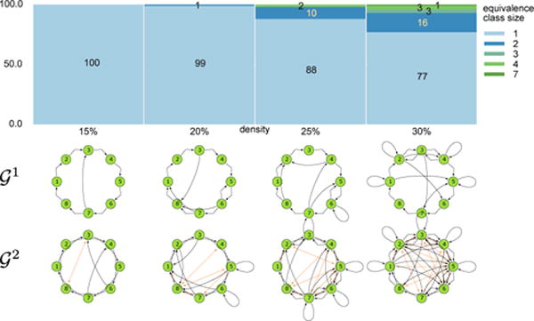
Equivalence class size distribution for 100 randomly generated 8-node SCCs at a given density and examples of 8-node SCCs for each of the densities.

Figure 7.

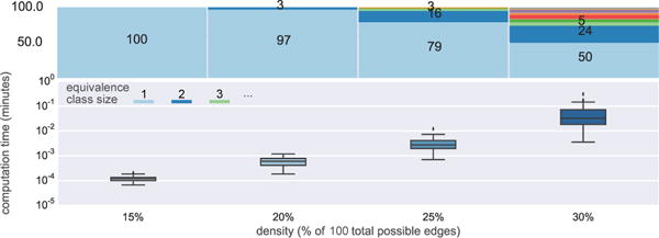
Distribution of run-time (wall clock) and sizes of equivalence classes across densities of 10-node graphs.

Figure 8.

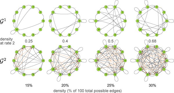
Example 10-node graphs at different densities and their corresponding ${\mathcal{G}}^1\mathrm{s}$.

The MSL algorithm is also computationally tractable for significantly larger n. For 15-node graphs, it can readily learn ${\mathcal{G}}^1$ structures up to 25% density, though outlier cases can take multiple days to compute. Figure 9 shows results for 100s of random SCCs with density of 10% for node sizes from 15 to 35. This density actually corresponds to quite challenging learning tasks. For example, a 35-node graph with 10% density can have nearly 400 edges in ${\mathcal{G}}^2$. Despite these large numbers of edges, the MSL algorithm rarely takes longer than an hour, even for 35-node graphs.

Figure 9.

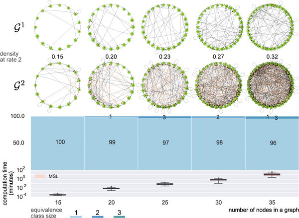
Graphs with 15, 20, 25, 30, and 35 nodes at the density of 10%, their corresponding ${\mathcal{G}}^2$ and equivalence class size distribution as well as the running time summarizing the computation of 100 random SCCs per node size.

4.2 Generality of the MSL algorithm

The MSL algorithm is actually an algorithm-schema that can be generalized to different known u, though its complexity rapidly increases. We performed a “proof-of-concept” of MSL for u = 3 with 100 random 6-node graphs. In this variant, each ${\mathcal{G}}^3$ edge has two virtual nodes that must be identified. Figure 10 shows the equivalence classes for u = 3. Interestingly, we obtain similar results with singleton equivalence classes dominating at low densities, but a rapid increase in the proportion of larger equivalence classes.

Figure 10.

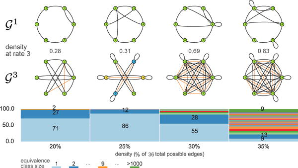
Applying the MSL algorithm to the ${\mathcal{G}}^3\to {\mathcal{G}}^1$ problem: results for 100 random 6 node graphs per density. Example ${\mathcal{G}}^1$ and their corresponding ${\mathcal{G}}^3$ are shown for reference.

4.3 Violations of the rate assumptions

If we know that u = 2, then MSL can successfully recover all graphs in the equivalence class. That assumption could easily be violated, however, as one might (for example) believe u = 2 when actually u = 3. Figure 11 shows results when MSL assuming u = 2 was applied to the ${\mathcal{G}}^3$ for 100 6-node graphs. Importantly, for ${\mathcal{G}}^1$ densities up to 30%, the MSL (assuming u = 2) algorithm fails to find a solution; that is, there is no ${\mathcal{G}}^1$ whose ${\mathcal{G}}^2$ matches the given graph (which is actually a ${\mathcal{G}}^3$). One can thus infer that a key algorithmic assumption has likely been violated. Unfortunately, the testability of the u = 2 assumption does not seem to extend to higher densities, which further suggests focusing our attention on ${\mathcal{G}}^1$ with no more than 30% density.

Figure 11.

Equivalence class size distribution for 100 randomly generated 6-node SCCs at a given density after the ${\mathcal{G}}^2\to {\mathcal{G}}^1$ MSL search when the input graph to the algorithm was in fact ${\mathcal{G}}^3$

4.4 From undersampled data to ${\mathcal{G}}^1$

The above results show that the nonparametric ${\mathcal{G}}^2\to {\mathcal{G}}^1$ component of the MSL algorithm is correct and computationally efficient, enabling us to learn equivalence classes for SCCs with densities up to 30%. For finite sample data, we need to incorporate a stable, reliable algorithm to learn the ℋ² structure. As noted earlier, there are multiple learning algorithms for this task (i.e., learning measurement-timescale structure), though they must allow for the possibility of bidirected edges to encode correlation between variables at the same time. We have used both a restricted version of the PC algorithm [11] and direct optimization of log likelihood in a structural vector autoregressive (SVAR) model [10]. In our experiments, we found that SVAR optimization provided more accurate and stable solutions, likely because of errors in conditional independence tests used in the modified PC algorithm. The best choice for learning ℋ² structure is an open research question. In the following, we only show results for the SVAR procedure.

We generated 100 random 8-node SCCs for each density in {15%, 20%, 25%, 30%}. These graphs are complex and interesting, but also are computationally tractable for the full MSL algorithm. For each random graph, we generated a random transition matrix by sampling weights for the non-zero elements of the adjacency matrix, and controlling system stability (by keeping the maximal eigenvalue at or below 1). This transition matrix was then used for a vector auto-regressive (VAR) model [10] with noise (standard deviation of 1) to generate data. Every other data sample was removed (to undersample at rate 2), and the resulting data was provided to the SVAR optimization to yield a candidate ℋ². The MSL algorithm was then applied to this ℋ² to obtain an equivalence class of ${\mathcal{G}}^1$ that can be compared to ground truth in terms of two error-types: omission error: the number of omitted edges normalized to the total number of edges in the ground truth; comission error: number of edges not present in the ground truth normalized to the total possible edges minus the number of those present in the ground truth. Figure 12 shows the results of these simulations. We also plot the estimation errors of the SVAR (on the undersampled data) to understand the dependence of MSL estimation errors on the estimation errors for ℋ². Interestingly, applying the MSL algorithm does not significantly increase the error rates over those produced by the SVAR estimation.

Figure 12.

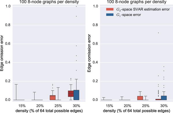
The MSL estimation and search errors on synthetic data undersampled at rate 2.

In some cases, SVAR estimation errors result in an ℋ² for which there are no possible ${\mathcal{G}}^1$.¹² For the simulations described in Figure 12, we deal with these cases by i) modifying MSL to accept (at the final step) those solutions that produce an undersampled graph that has the same directed edges as the estimated ℋ²; ii) restarting the simulation if a solution is not found. The former improves performance because bidirected edges often contain a weaker signal and are prone to mis-estimation, while the latter is to ensure comparability of results.

We have also modified the MSL algorithm so that, in these cases, it sequentially considers all neighbors of each ℋ² in the Hamming cube constructed on the length $n^2+\left(\begin{array}{c}n\\ 2\end{array}\right)$ binary string that represent directed and bidirected edges. If MSL finds a solution for one of these neighbors of ℋ², then we return it and compare to the ground truth as before.

We repeated our 8-node experiment successively checking neighborhoods from 1–5 steps away from the learned ℋ². In the worst case, this can require over 5.2 × 10⁷ additional MSL runs (for n = 8), so there can be a significant increase in run-time. The results are summarized in Figure 13. The increased complexity did not allow us to proceed to the 30% density. This time, however, we did not have to restart a single computation at densities or 15% and 20% with only few rejected at 25%.

Figure 13.

The estimation and search errors on synthetic data undersampled at rate 2 when the ${\mathcal{G}}^2$ Hamming cube neighborhood search is used.

5 Conclusions

Many scientific contexts depend on learning the structure of a system at some timescale that is faster than the measurement timescale. Standard structure learning algorithms can extract the measurement-level structure, but that structure can be quite different from the structure of the underlying system. The apparent structure given undersampled data is not immediately informative about the actual structure at the causal or system timescale. We have presented the first computationally efficient algorithm for learning the equivalence class of system-timescale structures that could have produced the measurement-timescale data. The algorithm can, in theory, be applied for arbitrary known undersample rates u, though it is computationally intractable for u > 3. Nonetheless, we have shown that the MSL algorithm exhibits promising performance for u = 2, including reliably learning underlying structure over large node-sets. The MSL algorithm also provides a novel tool for investigating the sizes of those equivalence classes. We showed that small amounts of undersampling typically do not destroy much information, as the equivalence class for many ${\mathcal{G}}^2$ was a singleton. Undersampling greatly increases the complexity of structure learning, but does not make it impossible or infeasible.

References

- 1.Chickering DM. Optimal structure identification with greedy search. The Journal of Machine Learning Research. 2003;3:507–554. [Google Scholar]
- 2.Danks D, Plis S. Learning causal structure from undersampled time series. JMLR: Workshop and Conference Proceedings. 2013;1:1–10. [Google Scholar]
- 3.Dash D. Restructuring dynamic causal systems in equilibrium. Proceedings of the Tenth International Workshop on Artificial Intelligence and Statistics (AIStats 2005) 2005:81–88. [Google Scholar]
- 4.Dean T, Kanazawa K. A model for reasoning about persistence and causation. Computational intelligence. 1989;5(2):142–150. [Google Scholar]
- 5.Fisher FM. A correspondence principle for simultaneous equation models. Econometrica: Journal of the Econometric Society. 1970:73–92. [Google Scholar]
- 6.Friedman N, Murphy K, Russell S. 15th Annual Conference on Uncertainty in Artificial Intelligence. San Francisco: Morgan Kaufmann; 1999. Learning the structure of dynamic probabilistic networks; pp. 139–147. [Google Scholar]
- 7.Granger CWJ. Investigating causal relations by econometric models and cross-spectral methods. Econometrica: Journal of the Econometric Society. 1969:424–438. [Google Scholar]
- 8.Huettel SA, Song AW, McCarthy G. Functional magnetic resonance imaging. Sinauer Associates, Publishers; Sunderland, MA, USA: 2004. [Google Scholar]
- 9.Iwasaki Y, Simon HA. Causality and model abstraction. Artificial Intelligence. 1994;67(1):143–194. [Google Scholar]
- 10.Lutkepohl H. New introduction to multiple time series analysis. Springer Science & Business Media; 2007. [Google Scholar]
- 11.Moneta A, Chlaß N, Entner D, Hoyer P. Causal search in structural vector autoregressive models. Journal of Machine Learning Research: Workshop and Conference Proceedings, Causality in Time Series (Proc NIPS2009 Mini-Symposium on Causality in Time Series) 2011;12:95–114. [Google Scholar]
- 12.Murphy K. PhD thesis, UC Berkeley. 2002. Dynamic Bayesian Networks: Representation, Inference and Learning. [Google Scholar]
- 13.Spirtes P, Glymour C, Scheines R. Causation, prediction, and search. Vol. 81. MIT press; 2001. [Google Scholar]
- 14.Thiesson B, Chickering D, Heckerman D, Meek C. Proceedings of the Twentieth Conference Annual Conference on Uncertainty in Artificial Intelligence (UAI-04) Arlington, Virginia: AUAI Press; 2004. Arma time-series modeling with graphical models; pp. 552–560. [Google Scholar]
- 15.Voortman M, Dash D, Druzdzel M. Proceedings of the Twenty-Sixth Annual Conference on Uncertainty in Artificial Intelligence (UAI) Corvallis, Oregon: AUAI Press; 2010. Learning why things change: The difference-based causality learner; pp. 641–650. [Google Scholar]
Associated Data
This section collects any data citations, data availability statements, or supplementary materials included in this article.