

Abstract
Mobile monitoring has provided a means for broad spatial measurements of air pollutants that are otherwise impractical to measure with multiple fixed site sampling strategies. However, the larger the mobile monitoring route the less temporally dense measurements become, which may limit the usefulness of short-term mobile monitoring for applications that require long-term averages. To investigate the stationarity of short-term mobile monitoring measurements, we calculated long term medians derived from a mobile monitoring campaign that also employed 2-week integrated passive sampler detectors (PSD) for NOx, Ozone, and nine volatile organic compounds at 43 intersections distributed across the entire city of Baltimore, MD. This is one of the largest mobile monitoring campaigns in terms of spatial extent undertaken at this time. The mobile platform made repeat measurements every third day at each intersection for 6–10 minutes at a resolution of 10 s. In two-week periods in both summer and winter seasons, each site was visited 3–4 times, and a temporal adjustment was applied to each dataset. We present the correlations between eight species measured using mobile monitoring and the 2-week PSD data and observe correlations between mobile NOx measurements and PSD NOx measurements in both summer and winter (Pearson’s r = 0.84 and 0.48, respectively). The summer season exhibited the strongest correlations between multiple pollutants, whereas the winter had comparatively few statistically significant correlations. In the summer CO was correlated with PSD pentanes (r = 0.81), and PSD NOx was correlated with mobile measurements of black carbon (r = 0.83), two ultrafine particle count measures (r =0.8), and intermodal (1–3 μm) particle counts (r = 0.73). Principal Component Analysis of the combined PSD and mobile monitoring data revealed multipollutant features consistent with light duty vehicle traffic, diesel exhaust and crankcase blow by. These features were more consistent with published source profiles traffic-related air pollutants than features based on the PSD data alone. Short-term mobile monitoring shows promise for capturing long-term spatial patterns of traffic-related air pollution, and is complementary to PSD sampling strategies.
Keywords: Traffic-related air pollution, mobile monitoring, ozone, ultrafine particles, black carbon
1. INTRODUCTION
Mobile monitoring has been commonly used to investigate the spatial distributions of traffic-related air pollutants (TRAP); however, mobile monitoring campaigns are resource intensive and are therefore typically limited in duration or require restricted spatial coverage to allow for both temporal and spatial density of data. A concern for using mobile monitoring data in a regulatory framework is establishing how representative short-term monitoring data are of longer-term spatial averages obtained by conventional methods. (Van den Bossche et al., 2015). To address this concern, we present an investigation into the stationarity of mobile monitoring data relative to fixed integrated passive sampler detectors (PSDs), as well as the added benefit of conducting both types of monitoring concurrently.
Both mobile monitoring and fixed sampler detection schemes (passive and continuous) have been used to refine predictive models for criteria pollutants and, more recently, for pollutants of emerging concern such as black carbon (Dons et al., 2013b) and ultrafine particle counts. Passive sampler detectors (PSD) adsorb air pollutants directly from the environment. PSDs are advantageous for their simplicity of use, and in the case of volatile organic compounds (VOCs), their ability to detect a large number of chemicals with a single sampler. However, the temporal resolution of PSDs is limited by analytical detection limits, and temperature-dependent sampling rates. When used for ambient monitoring PSDs typically require several days to collect a sample, and can be deployed for up to two weeks before saturation (Beckerman et al., 2008; Cohen et al., 2009).
Mobile monitoring platforms have now been developed for pedestrians (Marc et al., 2012) (Dons et al., 2013a), bicycles (Pattinson et al., 2014; Van den Bossche et al., 2015), trains (Castellini et al., 2014), and cars (Hudda et al., 2014; Pirjola et al., 2004). Mobile platforms can also be mobile labs consisting of trailers equipped with relatively simple portable instrumentation to highly sophisticated mass spectrometers (Massoli et al., 2012; Sun et al., 2012; von der Weiden-Reinmüller et al., 2014). Mobile monitoring provides real-time monitoring at a variety of locations, with the accompanying challenge of being temporally limited at any one place. It provides the means to measure air pollutant concentrations with broad spatial coverage using sophisticated equipment that would otherwise be impractical to duplicate in a fixed monitoring campaign.
Sullivan and Pryor (2014) used a combination of mobile monitoring and four continuous fixed site measurements to investigate the spatio-temporal variability of PM2.5 within a small urban region (~12 km). They found mobile monitoring provided enhanced spatial density whereas continuous fixed site monitors provided temporally-rich data. (Sullivan and Pryor, 2014). Other small spatial scale campaigns for black carbon and ultrafine particle counts have shown correlations between mobile routes in proximity to fixed sampling locations (Van den Bossche et al., 2015; Wu et al., 2015). All of these campaigns were limited in spatial extent due to the availability of fixed site locations and duplicate instrumentation both of which are logistically complicated to overcome. Duplication of instruments is resource intensive, which also restricts the number of pollutants measured and the ability to study pollutant mixtures.
In this work, we investigate the utility of combining readily deployed PSD and mobile monitoring. PSDs provide wide-spread spatial coverage for a dozen gaseous pollutants and mobile monitoring provides complimentary short-term measurements of both gaseous and particulate pollutants. Correlations between PSD and collocated continuous read measurements have been reported by Beckerman et al. in a previous near-roadway gradient study that consisted of a one week deployment of PSDs in Toronto, Canada (Beckerman et al., 2008). In our study, the sampling design consisted of mobile monitoring of eight pollutants in combination with 2-week fixed-site passive sampling of a combination of nine volatile organic compounds (VOCs), NO2, NOx, and ozone. The VOC speciation provided by the passive samplers allows differential detection of light duty (low molecular weight hydrocarbons) and heavy duty vehicles (long-chain alkanes) at each sampling location. In this study we selected forty-three monitoring locations in an approximately 400 km2 region encompassing the city and suburbs of Baltimore, MD making this one of the largest mobile monitoring campaigns in terms of spatial extent. Locations were selected to optimize spatial coverage near residences of participants in the Multi-Ethnic Study of Atherosclerosis (Cohen et al., 2009). Our two monitoring campaigns took place in February (winter) and June (summer) of 2012 to capture seasonal differences in pollutant distributions. We investigate both the pair-wise and multipollutant correlations between the two-week integrated PSD data and the 10-sec average mobile monitoring data in these two seasons.
2. METHODS
A detailed description of the methods for sample collection, sample analysis and statistical treatment of the data is provided in the supplementary material. In brief, two sampling campaigns were conducted in 2012 between February 12–22, 2012 and June18–27. The roadway intersections we selected throughout the urban area are depicted in Figure 1, representing a combination of residential streets and arterials with mixed traffic composition. PSDs positioned on utility poles near the intersections provided two-week integrated measures of various VOCs, ozone, NOx and NO2 as listed in Table 1. The PSD data were complemented by measurements obtained from a mobile platform (Riley et al., 2014) between the hours of 14:00–19:00 local time. Intersections were sampled along fixed routes every third day for a total of ~6–10 minutes at a sampling rate of 10 s. Each site was sampled 3–4 times during the summer and winter campaigns, and the order of the sampling was reversed each time the route was repeated We performed mobile monitoring continuously on the move (~20–35 km/hr), with each intersection and its surrounding area sampled in an alternating clover leaf pattern (Larson et al., 2009). We therefore use the term ‘roadway intersection’ to include an area several hundred meters in extent centered on a given intersection. Our mobile monitoring method therefore captures a distribution of air pollution concentrations at each intersection (Larson et al., 2009). The species used in this analysis are listed in Table 1 and the corresponding mobile instruments and their reporting ranges are provided in Table S1.
Figure 1.

Map of the study area. Fixed routes were driven for each colored subset of locations, with each route driven every third day. Map produced using ArcMap (ESRI Inc., 2014), railroad data from Open Baltimore, map layers from US census (Geography Division, 2008), and traffic counts from Maryland department of transportation (State Highway Administration, 2012).
Table 1.
List of species on mobile platform and passive sample detectors (PSD)
| Mobile Platform | PSD | ||
|---|---|---|---|
| Species | Units used | Species | Units used |
| UFPN (diameter 25–400 nm) | Counts/liter | Pentanes (includes pentanes and hexanes) | μg/m3multipy by 100 to achieve original conc. |
| PN1 (diameter 50–1000 nm) | Counts/liter | Benzene | μg/m3 |
| PNfine (diameter 0.25–1 μm) | Counts/liter | Toluene | μg/m3 |
| Intermodal PN (1–3 μm) | Counts/liter | m-Xylene | μg/m3 |
| Black Carbon (BC) | ng/m3 | o-Xylene | μg/m3 |
| NOx | ppb | Nonane | μg/m3 |
| CO (summer only)* | ppm | Decane | μg/m3 |
| O3 | mg/m3 | Undecane | μg/m3 |
| Volatile Organic Compounds (VOCs) | ppm | Dodecane (Winter Only)* | μg/m3 |
| NOx | ppb | ||
| NO2 | ppb | ||
| O3 | ppb | ||
Missing data in the case of winter CO, and laboratory error for summer Dodecane.
2.1 Mobile platform temporal adjustments
A central challenge to the use of mobile monitoring data for spatial analysis is developing methods to adjust for temporally-varying contributions to the observed values, such as day to day differences in meteorology that affect the entire region. For this analysis we are interested in determining how much each intersection typically differs from the well-mixed regional background levels as measured by the mobile platform during the study duration. Therefore, we processed the majority of mobile data to adjust for between-day temporal trends by subtracting the daily 5th percentile as discussed in the supplemental information section S4.2.
Mobile ozone measurements and PNFine (0.25–1 μm) contained within-day variability due to regional concentration changes (Supplemental S4.2.2 –S4.2.3). Thus we adjusted ozone and PNfine measurements by subtracting a 30-minute rolling 5th percentile (95th percentile for ozone), resulting in variables that are considered localized. The 30-minute window ensured that an area (~6 km2) larger than a single intersection (~0.36 km2) was used to estimate the background and the 5th percentile is reliably calculated from ~180 data points. We refer to the adjusted ozone concentrations as “ozone depletion”.
We then aggregated the adjusted mobile data at each roadway intersection across days within season, and calculated the median for each pollutant at each intersection. The median is obviously less sensitive than the mean to the presence of discrete high concentration plumes in the distribution of concentrations measured at an intersection. (Riley et al., 2014) The resultant medians are differential concentrations from the estimated daily or 30-minute rolling 5th percentile background concentrations. Therefore, a near zero or negative value is interpreted as an intersection whose measured concentrations were among the lowest recorded along each route. Figures S1 and S2 show that the distributions of concentrations recorded for the different routes were not systematically different from one another.
2.2 Mobile and PSD measurement correlations
Mobile data was then merged with the PSD data to generate the analysis dataset for each season. The resulting data files are available in the supplemental information. We calculated the Pearson’s correlation coefficients for the mobile data medians and the corresponding PSD 2-week averages, separately for each season. Because the PSD ozone measurements were uncorrelated with other pollutants we excluded them from the principal component analysis (PCA). We standardized the data by mean-centering and scaling by the variance, and calculated principal components from the correlation matrix using the function ‘principal’ from the R package “psych” (Revelle, 2015). We determined the number of components selected by requiring eigenvalues to be greater than one. To aid in interpretability of the components, we then rotated the selected components using Varimax.
3. RESULTS
3.1 Study area description
A map of the roadway intersections is provided in Figure 1. The map includes annual average weekday traffic counts, and train traffic routes. Environmentally critical areas of the sampling region include a 1 km perimeter along the port, where sites 1to 5 and site 43 are located. The port is serviced by a large number of low-traffic roads with high percentages of diesel truck traffic (truck traffic counts not shown). The roadway intersections are divided among the three different sampling routes; roadway intersection sites along the same route share common color shading.
3.2 Mobile data adjustments
Boxplots of the distribution of 10 s measurements taken at the roadway intersections are provided in the supplemental information (Figure S8–16) for both the unadjusted data as well as the adjusted data. The adjusted data were used to calculate the medians for each species at the roadway intersections for the two-week period, and the medians are indicated by the black dashed line in the figures. Black carbon (BC), ozone depletion, ultrafine particle number count (UFPN), and NOx all exhibit cross-season similarities in which specific roadway intersections had elevated concentrations of the respective species; for example, intersections in the downtown region are consistently elevated for pollutant concentrations as compared to the rest of the city. The spatial pattern is evident in the maps of the quintiles of the median concentrations for mobile species NOx, BC, and UFPN after data adjustment (Figure 2). The winter campaign took place during stronger winds than in summer with most days exhibiting a westerly direction (see Figures S17 and S18); this may account for higher concentrations of BC and UFPN on the eastern side of the city relative to summer which had no prevailing wind direction and lower wind speeds.
Figure 2.

Spatial distribution of pollutant quintiles for the mobile platform medians after data adjustment (concentrations represent the difference between the measured concentrations and the daily 5th percentile). Maps are a watercolor depiction of Baltimore, MD. Maps produced using the OpenStreetMap package in R (Fellows and Stotz, 2013).
3.3 PSD summary statistics
Boxplots for the PSD data are provided in Figure 3. The summer campaign had higher concentrations of each VOC species compared to the winter campaign (dodecane was excluded from the summer data due to high limit of detection from laboratory contamination). Both seasons exhibit a similar ranking of VOC concentrations: low molecular weight hydrocarbons had higher concentrations than the long chain alkanes ( > C6). Ozone concentrations were highest in the summer; conversely, oxides of nitrogen were higher in the winter consistent with observations at a nearby AQS monitor (see caption to Figure 3). The mobile monitoring platform also measured higher VOC and NOx concentrations in the summer compared to winter (see unadjusted data in the SI)
Figure 3.
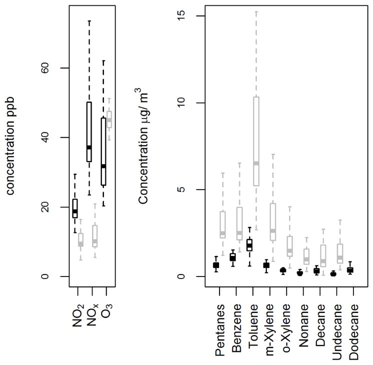
PSD summaries by analyte. Black (winter) and gray (summer). Pentanes are divided by 100 and include both pentanes and hexanes. For comparison AQS measurements taken in downtown Baltimore (GPS 39.298056, −76.604722) for NOx averaged 16.7 ppb in summer and 44.6 ppb in the winter over the same time period (U.S. Environmental Protection Agency Air Quality System (AQS) Data Mart, 2012). VOC data collected at the same location for the PAMS monitoring network indicates higher values in the winter rather than the summer for similar compounds. Benzene: 0.18 ppb summer (0.58 μg/m3), 0.37 ppb (1.18 μg/m3) winter. O-Xylene: 0.07 ppb summer (0.3 μg/m3), 0.06 ppb winter (0.26 μg/m3). Hexanes: 0.01 ppb summer (0.035 μg/m3), 0.33 ppb winter (1.16 μg/m3). AQS and PAMS data converted to μg/m3 assume standard temperature and pressure.
3.4 Mobile platform correlations
Scatterplot matrices for a subset of air pollutants measured by the mobile platform are presented in figure 4 for summer and winter. Histograms of concentrations show a tendency toward lower concentrations. The scatterplots generally follow a linear relationship in the summer, but a similarly clear trend is not evident in the winter. The correlation coefficients for the entire mobile dataset are provided in Tables 2 and 3 for summer and winter, respectively. Correlations are strongest between the particulate matter pollutants, and are stronger overall in the summer.
Figure 4.

Correlation scatterplot matrix for select mobile platform species for (A) summer and (B) winter. Pearson’s correlation coefficients are in the upper diagonal, values greater than 0.4 are significant (2-sided p = 0.01). Each data point represents the median derived from the sampling intersections. concentrations represent the difference between the measured concentrations and the daily 5th percentile.
Table 2.
Mobile Platform Pearson’s Correlation Coefficients, Summer
| UFPN | PN1 | PNFine | PN (1-3μm) | BC | NOx mob. | CO | O3 depl. | |
|---|---|---|---|---|---|---|---|---|
| UFPN | 0.94 | 0.77 | 0.82 | 0.84 | 0.8 | 0.33 | 0.8 | |
| PN1 | 0.94 | 0.72 | 0.8 | 0.84 | 0.86 | 0.28 | 0.78 | |
| PNFine | 0.77 | 0.72 | 0.84 | 0.74 | 0.59 | 0.25 | 0.75 | |
| PN (1-3μm) | 0.82 | 0.8 | 0.84 | 0.76 | 0.73 | 0.39 | 0.78 | |
| BC | 0.84 | 0.84 | 0.74 | 0.76 | 0.84 | 0.47 | 0.71 | |
| NOx mob. | 0.8 | 0.86 | 0.59 | 0.73 | 0.84 | 0.5 | 0.75 | |
| CO | 0.33 | 0.28 | 0.25 | 0.39 | 0.47 | 0.5 | 0.42 | |
| O3 depl. | 0.8 | 0.78 | 0.75 | 0.78 | 0.71 | 0.75 | 0.42 | |
| VOC | 0.52 | 0.48 | 0.44 | 0.57 | 0.52 | 0.47 | 0.49 | 0.43 |
The 2 sided probability p = 0.01 critical value for Pearson’s correlation coefficients is 0.40 for N = 40. The correlations coefficients are calculated using the medians derived for each sampling intersection after temporal adjustment as described in section 2.1.
Table 3.
Mobile Platform Pearson’s Correlation Coefficients, Winter
| UFPN | PN1 | PNFine | PN (1-3μm) | BC | NOx mob. | O3 depl. | |
|---|---|---|---|---|---|---|---|
| UFPN | 0.9 | 0.6 | 0.67 | 0.64 | 0.63 | 0.52 | |
| PN1 | 0.9 | 0.56 | 0.7 | 0.73 | 0.62 | 0.46 | |
| PNFine | 0.6 | 0.56 | 0.84 | 0.76 | 0.29 | 0.38 | |
| PN (1-3μm) | 0.67 | 0.7 | 0.84 | 0.88 | 0.41 | 0.3 | |
| BC | 0.64 | 0.73 | 0.76 | 0.88 | 0.33 | 0.29 | |
| NOx mob. | 0.63 | 0.62 | 0.29 | 0.41 | 0.33 | 0.32 | |
| O3 depl. | 0.52 | 0.46 | 0.38 | 0.3 | 0.29 | 0.32 | |
| VOC | −0.089 | −0.12 | −0.049 | −0.22 | −0.16 | −0.096 | 0.0061 |
The 2 sided probability p = 0.01 critical value for Pearson’s correlation coefficients is 0.40 for N = 40. The correlations coefficients are calculated using the medians derived for each sampling intersection after temporal adjustment as described in section 2.1.
3.5 PSD correlations
Scatterplot matrices for the subset of air pollutants measured by the PSDs are presented in figure 5 for summer and winter. The summer scatterplots follow the linear regression line reasonably well, but this is not observed in the winter except for a few cases (nonane and undecane). Histograms of PSD concentrations appear to be less skewed toward lower concentrations than those for the mobile platform data (Figure 4). The correlation coefficients for the entire PSD dataset are provided in Tables 4 and 5 for summer and winter respectively. The pollutants measured in summer were all significantly correlated (p = 0.01) except for PSD ozone. Correlations are weaker in the winter, and less than half of them are significant at p = 0.01.
Figure 5.

Correlation scatterplot matrix for select passive sampler detector species for (A) Summer and (B) winter. Pearson’s correlation coefficients are in the upper diagonal, values greater than 0.4 are significant (2-sided p = 0.01). Organic species have units of μg/m3, Pentanes have been divided by a factor of 100, and NOx has units of ppb.
Table 4.
PSD Pearson’s Correlation Coefficients, Summer
| Pentanes | Benzene | Toluene | m-Xylene | o-Xylene | Nonane | Decane | Undecane | NO2 | NOx | |
|---|---|---|---|---|---|---|---|---|---|---|
| Pentanes | 0.95 | 0.82 | 0.79 | 0.76 | 0.43 | 0.48 | 0.6 | 0.73 | 0.78 | |
| Benzene | 0.95 | 0.87 | 0.86 | 0.84 | 0.47 | 0.59 | 0.69 | 0.81 | 0.85 | |
| Toluene | 0.82 | 0.87 | 0.98 | 0.94 | 0.69 | 0.58 | 0.77 | 0.8 | 0.84 | |
| m-Xylene | 0.79 | 0.86 | 0.98 | 0.97 | 0.62 | 0.58 | 0.76 | 0.78 | 0.83 | |
| o-Xylene | 0.76 | 0.84 | 0.94 | 0.97 | 0.65 | 0.72 | 0.85 | 0.75 | 0.8 | |
| Nonane | 0.43 | 0.47 | 0.69 | 0.62 | 0.65 | 0.61 | 0.75 | 0.54 | 0.54 | |
| Decane | 0.48 | 0.59 | 0.58 | 0.58 | 0.72 | 0.61 | 0.91 | 0.48 | 0.47 | |
| Undecane | 0.6 | 0.69 | 0.77 | 0.76 | 0.85 | 0.75 | 0.91 | 0.62 | 0.61 | |
| NO2 | 0.73 | 0.81 | 0.8 | 0.78 | 0.75 | 0.54 | 0.48 | 0.62 | 0.96 | |
| NOx | 0.78 | 0.85 | 0.84 | 0.83 | 0.8 | 0.54 | 0.47 | 0.61 | 0.96 | |
| O3 | 0.39 | 0.44 | 0.25 | 0.24 | 0.23 | 0.024 | 0.17 | 0.16 | 0.45 | 0.46 |
The 2 sided probability p = 0.01 critical value for Pearson’s correlation coefficients is 0.40 for N = 40.
Table 5.
PSD Pearson’s Correlation Coefficients, Winter
| Pentanes | Benzene | Toluene | m-Xylene | o-Xylene | Nonane | Decane | Undecane | Dodecane | NO2 | NOx | |
|---|---|---|---|---|---|---|---|---|---|---|---|
| Pentanes | 0.38 | 0.26 | 0.44 | 0.45 | 0.31 | 0.054 | 0.32 | 0.022 | 0.084 | 0.27 | |
| Benzene | 0.38 | 0.43 | 0.47 | 0.46 | 0.35 | 0.22 | 0.44 | 0.15 | 0.43 | 0.51 | |
| Toluene | 0.26 | 0.43 | 0.51 | 0.5 | 0.29 | −0.004 | 0.25 | −0.061 | 0.19 | 0.43 | |
| m-Xylene | 0.44 | 0.47 | 0.51 | 0.99 | 0.76 | 0.39 | 0.74 | 0.3 | 0.49 | 0.79 | |
| o-Xylene | 0.45 | 0.46 | 0.5 | 0.99 | 0.78 | 0.38 | 0.75 | 0.29 | 0.49 | 0.79 | |
| Nonane | 0.31 | 0.35 | 0.29 | 0.76 | 0.78 | 0.48 | 0.87 | 0.32 | 0.5 | 0.64 | |
| Decane | 0.054 | 0.22 | −0.004 | 0.39 | 0.38 | 0.48 | 0.65 | 0.93 | 0.22 | 0.22 | |
| Undecane | 0.32 | 0.44 | 0.25 | 0.74 | 0.75 | 0.87 | 0.65 | 0.46 | 0.63 | 0.64 | |
| Dodecane | 0.022 | 0.15 | −0.061 | 0.3 | 0.29 | 0.32 | 0.93 | 0.46 | 0.068 | 0.12 | |
| NO2 | 0.084 | 0.43 | 0.19 | 0.49 | 0.49 | 0.5 | 0.22 | 0.63 | 0.068 | 0.76 | |
| NOx | 0.27 | 0.51 | 0.43 | 0.79 | 0.79 | 0.64 | 0.22 | 0.64 | 0.12 | 0.76 | |
| O3 | 0.1 | 0.28 | 0.27 | 0.077 | 0.065 | −0.1 | 0.039 | −0.13 | 0.2 | 0.014 | 0.2 |
The 2 sided probability p = 0.01 critical value for Pearson’s correlation coefficients is 0.40 for N = 40.
3.6 PSD vs. Mobile correlations
Scatterplot matrices between a subset of mobile monitoring medians and PSD data are provided in Figure 6. The scatterplots generally follow a linear regression for the summer campaign, but again not for the winter campaign. The correlation coefficients between the entire PSD and Mobile datasets are provided in Tables 6 and 7. The correlation matrix for summer reveals some high correlations between mobile platform and PSD data. In particular, CO has a higher correlation with PSD pentanes than it does with any mobile platform measurements which is also observed in the scatterplots. PSD NOx is highly correlated to mobile NOx and also with BC, UFPN and ozone depletion. Ozone depletion moderately correlated with PSD ozone as is mobile NOx. No other correlations are significant for PSD ozone in summer. The summer exhibited significant correlations between all mobile platform and PSD compounds except for PSD decane and ozone. In contrast, the majority of correlations observed in the winter between PSD and mobile data are insignificant (at p= 0.01). For seven of the monitoring days in winter, precipitation was recorded in the form of rain, snow, or fog. Winter wind speed averages exceeded 7 mph on 7 of the monitoring days with higher gusts (see figures S17–18). These meteorological factors may have resulted in increased deposition and dispersion of pollutants.
Figure 6.

Scatterplot matrix comparing select mobile platform and PSD species units provided in Table 1.
Table 6.
PSD vs. Mobile Pearson’s Correlation Coefficients, Summer
| UFPN | PN1 | PNFine | PN (1-3μm) | BC | NOx mob. | CO | O3 depl. | VOC | |
|---|---|---|---|---|---|---|---|---|---|
| Pentanes | 0.51 | 0.47 | 0.44 | 0.49 | 0.61 | 0.63 | 0.81 | 0.6 | 0.57 |
| Benzene | 0.62 | 0.6 | 0.51 | 0.58 | 0.7 | 0.74 | 0.73 | 0.67 | 0.54 |
| Toluene | 0.62 | 0.6 | 0.55 | 0.6 | 0.69 | 0.67 | 0.7 | 0.66 | 0.57 |
| m-Xylene | 0.62 | 0.61 | 0.54 | 0.61 | 0.67 | 0.67 | 0.65 | 0.65 | 0.53 |
| o-Xylene | 0.58 | 0.59 | 0.52 | 0.56 | 0.64 | 0.66 | 0.58 | 0.6 | 0.5 |
| Nonane | 0.42 | 0.38 | 0.44 | 0.36 | 0.5 | 0.38 | 0.46 | 0.4 | 0.42 |
| Decane | 0.36 | 0.37 | 0.27 | 0.29 | 0.41 | 0.48 | 0.27 | 0.31 | 0.39 |
| Undecane | 0.5 | 0.47 | 0.39 | 0.41 | 0.58 | 0.55 | 0.42 | 0.44 | 0.53 |
| NO2 | 0.79 | 0.77 | 0.69 | 0.71 | 0.83 | 0.83 | 0.58 | 0.77 | 0.44 |
| NOx | 0.82 | 0.8 | 0.71 | 0.73 | 0.83 | 0.84 | 0.59 | 0.8 | 0.51 |
| O3 | 0.38 | 0.37 | 0.33 | 0.28 | 0.39 | 0.49 | 0.32 | 0.55 | −0.081 |
The 2 sided probability p = 0.01 critical value for Pearson’s correlation coefficients is 0.40 for N = 40. The correlations coefficients are calculated between the PSD data and the medians derived for each sampling intersection after temporal adjustment of the mobile platform data as described in section 2.1.
Table 7.
PSD vs. Mobile Pearson Correlation Coefficients, Winter
| UFPN | PN1 | PNFine | PN (1-3μm) | BC | NOx mob. | O3 depl. | VOC | |
|---|---|---|---|---|---|---|---|---|
| Pentanes | 0.32 | 0.43 | 0.21 | 0.41 | 0.49 | 0.36 | −0.024 | −0.04 |
| Benzene | 0.3 | 0.23 | 0.16 | 0.12 | 0.19 | 0.19 | 0.33 | 0.22 |
| Toluene | 0.071 | 0.074 | -.034 | 0.074 | 0.095 | 0.031 | −0.14 | 0.12 |
| m-Xylene | 0.45 | 0.48 | 0.33 | 0.36 | 0.45 | 0.32 | 0.19 | 0.18 |
| o-Xylene | 0.42 | 0.45 | 0.33 | 0.36 | 0.44 | 0.3 | 0.19 | 0.18 |
| Nonane | 0.42 | 0.45 | 0.32 | 0.29 | 0.37 | 0.31 | 0.25 | 0.17 |
| Decane | 0.22 | 0.18 | 0.18 | 0.12 | 0.23 | 0.021 | 0.13 | 0.13 |
| Undecane | 0.48 | 0.47 | 0.48 | 0.38 | 0.42 | 0.28 | 0.31 | 0.26 |
| Dodecane | 0.064 | 0.064 | 0.078 | 0.035 | 0.15 | −0.062 | 0.083 | 0.096 |
| NO2 | 0.6 | 0.51 | 0.53 | 0.43 | 0.38 | 0.39 | 0.48 | 0.3 |
| NOx | 0.6 | 0.53 | 0.47 | 0.44 | 0.47 | 0.48 | 0.51 | 0.2 |
| O3 | −0.2 | −0.19 | -.064 | −0.08 | 0.073 | −0.18 | 0.13 | 0.08 |
The 2 sided probability p = 0.01 critical value for Pearson’s correlation coefficients is 0.40 for N = 40. The correlations coefficients are calculated between the PSD data and the medians derived for each sampling intersection after temporal adjustment of the mobile platform data as described in section 2.1.
The effect of the choice of temporal data adjustments on the correlation coefficients is presented in section S5.2 in the supplemental materials. We find that the daily 5th percentile adjustment gave the highest correlation between PSD and mobile data except for PNfine and ozone for which the rolling 30-minute 5th and 95th percentile adjustments (respectively) resulted in the highest correlations.
3.5 Principal component analysis
The rotated principal components (RC) are compared between PSD only data and combined PSD and mobile platform data in Figure 6 for the summer season only, where correlations between pollutants were strongest. Winter RCs were similar to the features derived for the summer dataset although they were not directly comparable due to the absence of mobile CO in the winter and dodecane in the summer. We excluded winter data from this analysis because bootstrap resampling of the winter data revealed that the RCs derived were unstable.
The PSD data yield two components that explain 87% of the total variability. One RC consists of high loadings for low molecular weight hydrocarbons, NO2, NOx, and the other RC has high loadings of long chain alkanes. Adding the mobile platform data results in three components with 83% of the total variance explained. Adding the mobile data further parses the low molecular weight VOC and NOx PSD data into two components instead of one. The correlations we observed between the mobile data and the PSD data are also evident in the first two components of the combined data analysis. In the combined dataset the first component has high loadings for particle counts, NOx mobile, and ozone depletion and PSD NOx and NO2, whereas the second component consists of CO highly correlated with low molecular weight hydrocarbons. The third component appears to be long chain VOCs that had little correlation to low molecular weight VOCs and the mobile data.
4. DISCUSSION
Whether or not short-term mobile monitoring data are representative of longer-term (2-week) measurements greatly impacts the utility of mobile monitoring campaigns in characterizing spatial patterns in air pollution. The first challenge in comparing mobile monitoring and PSD datasets is to define an appropriate measure of central tendency for the mobile monitoring species at each of the intersections, across the days of sampling. Our sampling scheme makes repeat measurements at roadway intersections every third day for a total of 3–4 visits lasting 6–10 minutes each. The distributions of measurements at a given intersection made on these separate days could differ depending upon temporally-varying factors such as traffic characteristics (weekend/weekday), meteorological factors (mixing height and wind speed and direction), and time of sampling (mid-afternoon versus evening/sundown). In this paper we chose to adjust the distributions to minimize between-day temporal variations in order to allow all other sources of variability to be aggregated over multiple days of sampling. Median values for each pollutant at each intersection were obtained from these aggregated distributions. Mobile platform measurements of absolute ozone concentration and absolute PNfine were excluded from this analysis because within-day variability due to meteorological or other non-local factors (regional transport) dominates the variability for these metrics (Wu et al., 2015) (Yli-Tuomi et al., 2005). For example, the boxplots for unadjusted PNfine and ozone concentrations (Figure S15–S16) compared to unadjusted BC (Figure S14) indicate that ozone concentrations are affected by both within and between day factors as evidenced by large daily concentration changes and vastly differing daily spatial patterns. In contrast consistent spatial patterns are observed in the quintiles of UFPN, BC, and NOx following data adjustment (see Figure 2). This choice of data adjustment is discussed in further detail in supplemental S4.2.
The VOCs measured on the PSD in winter were overall much lower in concentration than in the summer; however, the relative concentrations of the pollutants measured were similar in the two seasons indicating some consistency in the measurements. The Photochemical Assessment Monitoring Station (PAMS) data for Baltimore, which is located at the downtown AQS site, measured higher VOC concentrations in winter, and the concentrations were overall lower than what we measured on the PSDs. The PAMS data consists of one 24 hour sample every 6th day and therefore does not provide a direct comparison. The distribution of concentrations observed in winter is lower, which may account for the weaker correlations between VOCs in this season. PSD NOx and NO2 exhibit seasonal differences as well. In the summer, NOx and NO2 have nearly identical distributions of concentrations (see Figure 2) and are correlated with r = 0.96, whereas in winter, NOx is almost twice the concentration of NO2 and the correlation is r = 0.76. This indicates that NOx in summer is almost entirely NO2, whereas in winter NO makes up a substantial amount of NOx concentrations.
The only pollutant common to both the PSD and mobile monitoring sampling was NOx, and the scatterplot matrices in Figure 6 illustrate that the mobile monitoring and PSD measures were correlated for this pollutant, especially during the summer campaign. This result indicates that source activity that was sampled briefly by mobile monitoring in four afternoon visits distributed across two weeks is relevant to the source activity sampled over the entire two weeks. The strong correlation between PSD pentanes and mobile CO in the summer campaign is particularly noteworthy because these combined measurements indicate that the sampling strategy is detecting VOCs arising from mobile sources (in US cities ~95% of CO is emitted from vehicles). (U.S. EPA, 2008) The presence of significant correlation between a the PSDs and adjusted mobile platform measurements suggests that the comparatively limited amount of time sampling at each site by the mobile platform averaged across multiple visits is in fact representative of longer-term spatial contrasts between locations within a city (Figure 2). This observation is particularly helpful for interpreting particle count distributions as well as BC measurements for which there so far have been few low-cost solutions for obtaining multiple, simultaneous, fixed site, time-integrated measurements.
The correlation results (especially from summer) are consistent with previous campaigns comparing mobile data to fixed site and near roadway monitors. Typically it is found that the mobile platform concentrations are most correlated with the fixed site measurements collected nearest to the mobile route. (Sullivan and Pryor, 2014; Van den Bossche et al., 2015) Beckerman et al reported correlations between continuous read measurements (ultrafine particle mass and PM2.5) and 1 week PSD (Ogawa and 3M) measurements of NO2, NOx, ozone, benzene, xylenes, and hexanes (among other VOCs) in a colocation experiment measuring the near road gradient of two major highways (Beckerman et al., 2008). They report similar correlation coefficients to our summer campaign (between 0.6 and 0.8), although they have fewer points of comparison and their monitor placements were measuring the same source. Our correlations between UFPN and VOCs are also similar to those reported from a near-roadway gradient measurement made by real-time instruments in a summer campaign in Raleigh, North Carolina (Hagler et al., 2009). Correlations between pollutants on mobile platforms have also been found to vary by neighborhood in some studies with correlation coefficients ranging between 0.35–0.8 between particle number counts and NOx (Patton et al., 2014), which may indicate variation in traffic characteristics.
The principal components analysis on the PSD-only data resulted in two components compared to three for the combined PSD and mobile analysis for the summer. The PSD-only rotated components reveal that the majority of the variance is described by a feature enriched in low molecular weight hydrocarbons and NOx. However, with the addition of the mobile platform measurements, the VOC and NOx data are split among three features. The strong correlations between the PSD NOx measures and the mobile platform NOx, BC, and particulate matter species are revealed in the first component. Whereas the strong correlations between mobile CO and the low molecular weight hydrocarbons appear in the second feature. Finally, the least amount of variance is attributed to the high molecular weight hydrocarbon feature, RC3. Our findings are similar to Oakes and colleagues, who found that NOx was approximately evenly split between multipollutant features they designated as diesel, gasoline, and “total mobile sources”. (Oakes et al., 2014). RC1 for the combined data has loadings consistent with emission factors for diesel exhaust (Hudda et al., 2013; Westerdahl et al., 2005). RC2 has high loadings of mobile CO and lower molecular weight hydrocarbons as well as mobile and PSD NOx; this feature is consistent with light duty vehicle traffic (Hudda et al., 2013; Oakes et al., 2014). Finally, RC3 is enhanced in the longer chain alkanes (n > 6) that are uncorrelated with both PN and BC concentrations, typical of uncontrolled crankcase emissions from diesel engine road-draft tubes (Zielinska et al., 2008).
This work only used mobile sampling in the afternoon, which is a potential limitation of this study particularly in winter when 1–3 hours of sampling occurs after dark. Also the PSD samplers capture the morning commute in addition to the afternoon commute, which might also be an important factor for correlations between PSD and mobile measurements in winter. In summer, we note, that correlations between PSD and mobile measurements exceed 0.8 which indicates the mobile platform sampling strategy is capturing the spatial variability in this season. In summer, the absence of a prevailing wind direction over the duration of the two-week period was serendipitous as the concentrations at intersections near highways would ordinarily be impacted by downwind transport. The weaker correlations in winter (including PSD only) were unexpected since winter typically exhibits stronger correlations between air pollutants as has been reported by Patton et al. (2014).. Typically higher correlations in winter have been attributed to increased atmospheric stability. We speculate several days of precipitation and strong winds during the winter campaign may have contributed to the weaker correlations for both PSD and mobile measurements. Therefore, the generalizability of the correlation results for the two week period of the campaign to the remainder of winter is questionable.
5. CONCLUSIONS
We have presented an analysis of the correlations between long-term integrated PSD data and short-term, time resolved mobile monitoring data. The correlations we observed between the PSD and mobile measurements demonstrated that underlying spatial variability in specific TRAP components could be reliably captured in a relatively short total measurement time at each location, provided those measurements were aggregated over several days, and that the data are appropriately adjusted for between day changes in background concentrations of each component. This is particularly helpful in that several of the pollutants monitored with the mobile platform (e.g. BC, PN1) cannot be measured with inexpensive PSDs. In addition, for pollutants where regional transport dominates the variance in concentrations (ozone and PM2.5), a 30-minute moving 5th percentile (or 95th percentile for ozone) sufficiently isolates the local contribution to observed concentrations.
It is not straightforward to adjust for confounding temporal factors in a spatially and temporally varying dataset. For interested readers, we’ve included a more detailed discussion of how the correlation results change with choice of temporal correction in the supplement section S.5.2. Finally, a PCA of the combined PSD and mobile monitoring data revealed a number of multipollutant mixtures, and these features were more consistent with published source profiles for TRAP, compared to an analysis based on the PSD data alone.
Supplementary Material
Figure 7.

Summer season principal component analyses with varimax rotation for PSD data and the combined mobile medians and PSD data, respectively. Loadings of rotated components (RC) are depicted. Breakdown of variance explained PSD only: RC1PSD 53% and RC2PSD 34%. Combined mobile and PSD: RC1 37%, RC2 25% and RC3 22% (Total 83%).
HIGHLIGHTS.
A city wide mobile monitoring campaign was combined with passive samplers
Correlations between mobile and passive measurements were moderate to strong
Short term mobile monitoring may be representative of long term spatial patterns.
Acknowledgments
This publication was made possible by USEPA grant (RD-83479601-0). Its contents are solely the responsibility of the grantee and do not necessarily represent the official views of the USEPA. Further, USEPA does not endorse the purchase of any commercial products or services mentioned in the publication. Additional support provided by the National Institute of Environmental Health Sciences (T32ES015459, P30ES007033). This publication’s contents are solely the responsibility of the authors and do not necessarily represent the official views of the sponsoring agencies. Laboratory analysis of the 3M passive sampler detectors was performed by the Environmental Health Laboratory at the University of Washington under direction of Dr. Russell Dills.
Footnotes
Publisher's Disclaimer: This is a PDF file of an unedited manuscript that has been accepted for publication. As a service to our customers we are providing this early version of the manuscript. The manuscript will undergo copyediting, typesetting, and review of the resulting proof before it is published in its final citable form. Please note that during the production process errors may be discovered which could affect the content, and all legal disclaimers that apply to the journal pertain.
References
- Beckerman B, Jerrett M, Brook JR, Verma DK, Arain MA, Finkelstein MM. Correlation of nitrogen dioxide with other traffic pollutants near a major expressway. Atmos Environ. 2008;42(2):275–290. [Google Scholar]
- Castellini S, Moroni B, Cappelletti D. PMetro: Measurement of urban aerosols on a mobile platform. Measurement. 2014;49:99–106. [Google Scholar]
- City of Baltimore. Open Baltimore. Shape file Baltimore railroad. 2008 https://data.baltimorecity.gov/browse?category=Geographic.
- Cohen MA, Adar SD, Allen RW, Avol E, Curl CL, Gould T, Hardie D, Ho A, Kinney P, Larson TV, Sampson P, Sheppard L, Stukovsky KD, Swan SS, Liu LJS, Kaufman JD. Approach to Estimating Participant Pollutant Exposures in the Multi-Ethnic Study of Atherosclerosis and Air Pollution (MESA Air) Environ Sci Technol. 2009;43(13):4687–4693. doi: 10.1021/es8030837. [DOI] [PMC free article] [PubMed] [Google Scholar]
- Dons E, Temmerman P, Van Poppel M, Bellemans T, Wets G, Panis LI. Street characteristics and traffic factors determining road users’ exposure to black carbon. Sci Total Environ. 2013a;447:72–79. doi: 10.1016/j.scitotenv.2012.12.076. [DOI] [PubMed] [Google Scholar]
- Dons E, Van Poppel M, Kochan B, Wets G, Int Panis L. Modeling temporal and spatial variability of traffic-related air pollution: Hourly land use regression models for black carbon. Atmos Environ. 2013b;74:237–246. [Google Scholar]
- ESRI Inc. ArcGIS: ArcMap. 2014. 10.2.2.3552. [Google Scholar]
- Fellows I, Stotz JP. OpenStreetMap: Access to open street map raster images. 2013. 0.3.1. [Google Scholar]
- Geography Division, U.S. Department of Commerce (U.S. Census Bureau) TIGER/Line Shapefile, 2008, county. Baltimore city, MD (24510): 2008. http://www.census.gov/geo/maps-data/data/tiger-line.html. [Google Scholar]
- Hagler GSW, Baldauf RW, Thoma ED, Long TR, Snow RF, Kinsey JS, Oudejans L, Gullett BK. Ultrafine particles near a major roadway in Raleigh, North Carolina: Downwind attenuation and correlation with traffic-related pollutants. Atmos Environ. 2009;43(6):1229–1234. [Google Scholar]
- Hudda N, Fruin S, Delfino RJ, Sioutas C. Efficient determination of vehicle emission factors by fuel use category using on-road measurements: downward trends on Los Angeles freight corridor I-710. Atmospheric Chemistry and Physics. 2013;13(1):347–357. doi: 10.5194/acp-13-347-2013. [DOI] [PMC free article] [PubMed] [Google Scholar]
- Hudda N, Gould T, Hartin K, Larson TV, Fruin SA. Emissions from an International Airport Increase Particle Number Concentrations 4-fold at 10 km Downwind. Environ Sci Technol. 2014;48(12):6628–6635. doi: 10.1021/es5001566. [DOI] [PMC free article] [PubMed] [Google Scholar]
- Larson T, Henderson SB, Brauer M. Mobile Monitoring of Particle Light Absorption Coefficient in an Urban Area as a Basis for Land Use Regression. Environ Sci Technol. 2009;43(13):4672–4678. doi: 10.1021/es803068e. [DOI] [PubMed] [Google Scholar]
- Marc M, Zabiegala B, Namiesnik J. Mobile Systems (Portable, Handheld, Transportable) for Monitoring Air Pollution. Crit Rev Anal Chem. 2012;42(1):2–15. [Google Scholar]
- Massoli P, Fortner EC, Canagaratna MR, Williams LR, Zhang Q, Sun Y, Schwab JJ, Trimborn A, Onasch TB, Demerjian KL, Kolb CE, Worsnop DR, Jayne JT. Pollution Gradients and Chemical Characterization of Particulate Matter from Vehicular Traffic near Major Roadways: Results from the 2009 Queens College Air Quality Study in NYC. Aerosol Sci Technol. 2012;46(11):1201–1218. [Google Scholar]
- Oakes MM, Baxter LK, Duvall RM, Madden M, Xie MJ, Hannigan MP, Peel JL, Pachon JE, Balachandran S, Russell A, Long TC. Comparing Multipollutant Emissions-Based Mobile Source Indicators to Other Single Pollutant and Multipollutant Indicators in Different Urban Areas. Int J Env Res Public Health. 2014;11(11):11727–11752. doi: 10.3390/ijerph111111727. [DOI] [PMC free article] [PubMed] [Google Scholar]
- Pattinson W, Longley I, Kingham S. Using mobile monitoring to visualise diurnal variation of traffic pollutants across two near-highway neighbourhoods. Atmos Environ. 2014;94(0):782–792. [Google Scholar]
- Patton AP, Perkins J, Zamore W, Levy JI, Brugge D, Durant JL. Spatial and temporal differences in traffic-related air pollution in three urban neighborhoods near an interstate highway. Atmos Environ. 2014;99:309–321. doi: 10.1016/j.atmosenv.2014.09.072. [DOI] [PMC free article] [PubMed] [Google Scholar]
- Pirjola L, Parviainen H, Hussein T, Valli A, Hameri K, Aaalto P, Virtanen A, Keskinen J, Pakkanen TA, Makela T, Hillamo RE. “Sniffer” - a novel tool for chasing vehicles and measuring traffic pollutants. Atmos Environ. 2004;38(22):3625–3635. [Google Scholar]
- Revelle W. psych: Procedures for Personality and Psychological Research. Northwestern University; Evanston, Illinois, USA: 2015. 1.5.6. [Google Scholar]
- Riley EA, Banks L, Fintzi J, Gould TR, Hartin K, Schaal L, Davey M, Sheppard L, Larson T, Yost MG, Simpson CD. Multi-pollutant mobile platform measurements of air pollutants adjacent to a major roadway. Atmos Environ. 2014;98(0):492–499. doi: 10.1016/j.atmosenv.2014.09.018. [DOI] [PMC free article] [PubMed] [Google Scholar]
- State Highway Administration, Maryland Department of transportation. Annual Average Daily Traffic Counts. 2012 http://sha.maryland.gov/pages/GIS.aspx?PageId=838.
- Sullivan R, Pryor S. Quantifying spatiotemporal variability of fine particles in an urban environment using combined fixed and mobile measurements. Atmos Environ. 2014;89:664–671. [Google Scholar]
- Sun YL, Zhang Q, Schwab JJ, Chen WN, Bae MS, Hung HM, Lin YC, Ng NL, Jayne J, Massoli P, Williams LR, Demerjian KL. Characterization of near-highway submicron aerosols in New York City with a high-resolution aerosol mass spectrometer. Atmospheric Chemistry and Physics. 2012;12(4):2215–2227. [Google Scholar]
- U.S. Environmental Protection Agency Air Quality System (AQS) Data Mart. [July 2013];EPA AQS Data for Oldtown Fire Station, 1100 Hillen Street. 2012 http://www.epa.gov/ttn/airs/aqsdatamart/access/interface.htm.
- U.S. EPA. Latest findings on national air quality: Status and trends through 2006, EPA-454/R-07-007. Research Triangle Park, NC: 2008. p. 22. [Google Scholar]
- Van den Bossche J, Peters J, Verwaeren J, Botteldooren D, Theunis J, De Baets B. Mobile monitoring for mapping spatial variation in urban air quality: development and validation of a methodology based on an extensive dataset. Atmos Environ 2015 [Google Scholar]
- von der Weiden-Reinmüller SL, Drewnick F, Zhang QJ, Freutel F, Beekmann M, Borrmann S. Megacity emission plume characteristics in summer and winter investigated by mobile aerosol and trace gas measurements: the Paris metropolitan area. Atmos Chem Phys. 2014;14(23):12931–12950. [Google Scholar]
- Westerdahl D, Fruin S, Sax T, Fine PM, Sioutas C. Mobile platform measurements of ultrafine particles and associated pollutant concentrations on freeways and residential streets in Los Angeles. Atmos Environ. 2005;39(20):3597–3610. [Google Scholar]
- Wu H, Reis S, Lin C, Beverland IJ, Heal MR. Identifying drivers for the intra-urban spatial variability of airborne particulate matter components and their interrelationships. Atmos Environ. 2015;112:306–316. [Google Scholar]
- Yli-Tuomi T, Aarnio P, Pirjola L, Makela T, Hillamo R, Jantunen M. Emissions of fine particles, NOx, and CO from on-road vehicles in Finland. Atmos Environ. 2005;39(35):6696–6706. [Google Scholar]
- Zielinska B, Campbell D, Lawson DR, Ireson RG, Weaver CS, Hesterberg TW, Larson T, Davey M, Liu LJS. Detailed Characterization and Profiles of Crankcase and Diesel Particular Matter Exhaust Emissions Using Speciated Organics. Environ Sci Technol. 2008;42(15):5661–5666. doi: 10.1021/es703065h. [DOI] [PMC free article] [PubMed] [Google Scholar]
Associated Data
This section collects any data citations, data availability statements, or supplementary materials included in this article.