Metabolomics by Gas Chromatography-Mass Spectrometry: the combination of targeted and untargeted profiling

Abstract

Gas chromatography-mass spectrometry (GC-MS)-based metabolomics is ideal for identifying and quantitating small molecular metabolites (<650 daltons), including small acids, alcohols, hydroxyl acids, amino acids, sugars, fatty acids, sterols, catecholamines, drugs, and toxins, often using chemical derivatization to make these compounds volatile enough for gas chromatography. This unit shows that on GC-MS- based metabolomics easily allows integrating targeted assays for absolute quantification of specific metabolites with untargeted metabolomics to discover novel compounds. Complemented by database annotations using large spectral libraries and validated, standardized standard operating procedures, GC-MS can identify and semi-quantify over 200 compounds per study in human body fluids (e.g., plasma, urine or stool) samples. Deconvolution software enables detection of more than 300 additional unidentified signals that can be annotated through accurate mass instruments with appropriate data processing workflows, similar to liquid chromatography-MS untargeted profiling (LC-MS). Hence, GC-MS is a mature technology that not only uses classic detectors (‘quadrupole’) but also target mass spectrometers (‘triple quadrupole’) and accurate mass instruments (‘quadrupole-time of flight’). This unit covers the following aspects of GC-MS-based metabolomics: (i) sample preparation from mammalian samples, (ii) acquisition of data, (iii) quality control, and (iv) data processing.

Introduction

Gas chromatography–mass spectrometry (GC-MS) is the most standardized method in metabolomics, with almost 50 years of established protocols for metabolite analyses (e.g., sugars (DeJongh et al, 1969), amino acids (Gelpi et al, 1969), sterols (Brooks et al, 1968), hormones (Gréen, 1969), catecholamines (Anggard & Sedvall, 1969), hydroxyl acids (Kuksis & Prioreschi, 1967), fatty acids (Niehaus Jr & Ryhage, 1968), aromatics (Coward & Smith, 1969) and many other intermediates of primary metabolism. Indeed, the intriguing possibility to combine such targeted analysis of specific compound classes into profiling assays for large swaths of metabolism was first accomplished by GC-MS in the 1970s, including the use of such profiles to improve diagnosis of human diseases (Thompson & Markey, 1975), using 140 subjects or more (Zlatkis et al, 1973). Today, we call such profiling “metabolomics” to emphasize the need to identify and quantify all small molecules that are present in a given biological situation, and to use such profiles as output of the cellular machinery in response to genetic or environmental perturbations (Fiehn, 2002).

For over 40 years, mass spectra and chromatographic retention times have been accumulated in publicly available libraries under standardized conditions of 70 eV electron ionization energy, most notably in the NIST 14 Mass Spectral Library collection of the U.S. National Institute of Standards and Technology (NIST) (Babushok et al, 2007), but also larger, less well curated versions (e.g., the Wiley registry (Roessner et al, 2000), the open-access MassBank database (Horai et al, 2010), and the Golm repository (Kopka et al, 2005)). Similarly, efforts to computationally match mass spectral records to experimental data (McLafferty et al, 1974), and to interpret mass spectra for compound identifications, started in the 1960 (Venkataraghavan et al, 1969) and are still ongoing (Ma et al, 2014), (Fiehn et al, 2000b), (Kumari et al, 2011). The NIST14 library comprises GC-MS mass spectra for 242,477 unique compounds of which roughly one third have recorded standardized retention times, enabling the use of two orthogonal parameters (mass spectral and retention index matching) for compound identification. In comparison, LC-MS/MS spectral libraries are significantly smaller in size, with only 8,171 unique compounds in the NIST14 library or 12,099 unique compounds in the Metlin LC-MS/MS library (which lack retention information).

In addition to these standardized libraries, GC-MS has specific advantages that led to labeling this technology as the “gold standard” in metabolomics (Lu et al, 2008), i.e., the method against which newer approaches should be compared to with respect to breadth, sensitivity and specificity of metabolite detections. Most notably, electron ionization leads to complex and rich fragmentation patterns which can be exploited to increase the specificity in mass spectral matching, especially if these mass spectra are recorded in large user libraries with standardized protocols for data acquisition such as in the Fiehnlib libraries (Kind et al, 2009) and the BinBase databases (Fiehn et al, 2005), (Skogerson et al, 2011). Peak picking is therefore accompanied by true mass spectral deconvolution that summarize all fragment ions into purified mass spectra, unlike to LC-MS approaches in which MS and data dependent MS/MS fragmentations are used separately. Automated mass spectral deconvolution software (AMDIS) is freely available for GC-MS, since 1998 (Stein, 1999), and has been successfully in use for metabolomics since that time (Halket et al, 1999), (Fiehn et al, 2000a). Similar attempts to couple ionization with fragmentation in LC-MS in an untargeted manner have recently started, for example using SWATH approaches (Hopfgartner et al, 2012), but at current, there is no open-access software for LC-MS that is as capable of purifying mass spectra of co-eluting mass spectra in GC-MS (e.g., AMDIS) or its commercial versions (e.g., ChromaTOF) (Lee et al, 2012).

Strategic Planning

Metabolomics based on GC-MS is best suited by focusing extraction and sample preparation procedures to compound classes that are most amenable to GC-MS, while discarding metabolic classes that could potentially lead to matrix problems or memory effects, hence compromising data quality. First of all, simple logic dictates that volatiles, such as targeted for breath analysis in lung cancer (Buszewski et al, 2012) or for emission of compounds from plants, can only be analyzed by gas chromatography (Roach et al, 2014), but not by liquid chromatography. There are a number of options to pursue metabolomics for volatile profiling, from simple headspace injections (Tikunov et al, 2005) to enrichment of volatiles on adsorption materials, followed by thermal desorption into GC/MS instruments, notably by solid phase microextractions (SPME) that can also be used for fecal matter to study gut microbiome/health interactions (Dixon et al, 2011), by active adsorption techniques that better control sample collections and hence, can give precise absolute quantifications (Zhang & Li, 2010), or by passive adsorption using materials that have much larger capacity than SPME fibers (Aksenov et al, 2014). However, in comparison to use of GC-MS for metabolomics of primary metabolism such as sugars, amino acids, hydroxyl acids and related biochemical pathways, volatile profiling is used less frequently and is mostly constrained to plant research.

Therefore, protocols given here focus on such standard pathway metabolomics, and do not detail differences in procedures for profiling of volatiles. Indeed, volatiles are usually discarded in most GC-MS or LC-MS assays because most protocols utilize steps in which samples are either desiccated under vacuum or under a gentle stream of nitrogen, both of which invariably lose volatile compounds such as acetic acid, acetone or other low-boiling compounds. As most primary metabolites have higher boiling points, for example, lactate, pyruvate, malic acid, glucose, palmitate or similar metabolites, GC-MS requires a derivatization step to render these compounds volatile enough for analysis. The most common derivatization protocol uses trimethylsilylation (Kumari et al, 2011), (Fiehn et al, 2010) or variants thereof like tert.butydimethylsilylation (Niehaus et al, 2014), (Fiehn et al, 2000b), both of which remove acidic protons from hydroxyl-, carboxyl-, amino- or thiol-groups. These derivatization reactions are performed under very mild conditions, work fast and with extraordinary high yields, breaking molecular proton bridge bonding and hence, decrease boiling points and increase stability of compounds for GC-MS analysis (Laine & Sweeley, 1971). In general, silylation reactions are more universal and easier to perform than alternative reactions such as methylations, although some reports point to complementary strategies such as using ethyl chloroformates (Gao et al, 2009). There is a plethora of literature on optimal extraction procedures for metabolomics (Trygg et al, 2005), (Fiehn & Kind, 2007), including for GC-MS based metabolomics. However, the truth is, there is no optimal procedure: there are only compromises that are more, or less, suitable for specific molecular targets given the complexity of biological matrices, metabolite enzymatic turnover rates, or the need to enrich low abundant compounds. For example, if methanol is used for extractions, lipids (including the abundance of triacylglycerides and phospholipids!) are extracted in substantial amounts from biological materials. Such lipids are involatile in GC-MS under trimethylsilylating conditions and would, hence, accumulate in the injection interface used in GC-MS, called the ‘liner’. As lipids accumulate in these liners, portions of these lipids get pyrolyzed in the hot injection conditions in GC-MS, leading to increasing amounts of (mostly saturated) carry-over background fatty acid signals detected in the chromatograms (Fiehn et al, 2008). Conversely, if researchers only use water (or hot water) for metabolomics extractions, sugars and hydroxyl acids would be completely extracted while lipids would remain in the pellets. However, ranges of mid-polarity compounds, from sterols to aromatics, would not be exhaustively extracted under these conditions.

Therefore, the protocol below uses a ternary combination of hydrophilic (water) and lipophilic (isopropanol) solvents with acetonitrile as medium polarity solvent (Yerges-Armstrong et al, 2013). To remove very lipophilic lipids, the protocol employs a clean-up step after the initial extraction and desiccation (Fiehn et al, 2008). We have noted that if such lipid clean-up step is not employed, trimethylsilylation reactions may be hampered for amino acids and polyamines, for example for postprandial blood plasma samples after lipid-rich meals. The protocol listed below is under frequent evaluation and comparison to alternative mixtures, temperatures and protocols. To this point, the isopropanol/acetonitrile/water extraction protocol has consistently outperformed all other protocols with respect to analytical precision (i.e., relative standard deviation) and comprehensiveness (presence of all metabolites typically detected in mammalian samples). Unfortunately, this comparison is also true for a direct evaluation of the Fiehnlab Standard Operating Procedure (SOP) against the lipidomics Matyash protocol (Matyash et al, 2008) that efficiently extracts lipids in its methyl-tert.butyl ether layer, and for which we have used the corresponding water/methanol layer for GC-MS profiling. Nevertheless, using the Matyash protocol and employing the polar phase for GC-MS profiling of primary metabolites is still a good alternative if limited amount of material is available, i.e. when researchers are forced to choose one specific extraction and fractionation method instead of best-suited protocols that have been developed for specific matrices.

It is important to note, though, that for plant samples, an alternative extraction protocol is used employing chloroform/methanol/water (2/5/2, volumetric ratios) (Fiehn et al, 2008). Using the isopropanol-based protocol is more suitable for mammalian or cell samples, including blood plasma, urine, or tissue samples. Interestingly, however, in plant samples, specific compounds show severe decrease in intensity in comparative evaluations using the isopropanol-based extraction mixture, such as cysteine or ascorbate. The reader is therefore advised to perform comparative extraction evaluation whenever novel matrices are targeted for metabolomics assessments, or when large-scale analyses require utmost scrutiny for long-term reliability.

Basic Protocol 1: Sample preparation of mammalian samples for GC-MS metabolome analysis

Introduction

This Basic Protocol describes sample extraction and sample preparation for primary metabolism profiling by gas chromatography/mass spectrometry (GC-quadrupole (Q) MS or GC-time of flight (TOF) MS). Roughly 95% of the instruments on the market are GC-quadrupole MS instruments as inexpensive mass spectrometers with slow scanning capabilities and unit mass resolution. Alternatively, several vendors also sell high resolution GC-QTOF MS instruments for accurate mass determination for elucidating unknown peaks. The company Leco further sells GC-TOF MS instruments with very fast data acquisition capabilities and full mass spectral deconvolution software, but unit resolution. Data acquisition quality control procedures refer to all instruments. Data curation result sheets are exemplified for Leco GC-TOF MS instrument results but can be extended for result sheets obtained by adequate alternative software or data processing schemes.

All parameters have a validation range of 10% of the given set point. However, for several parameters it can be expected that the SOP also sufficiently performs in larger deviation areas from the given set points. The SOP has been used in a wide area of different matrices, most importantly in blood, for which the author’s laboratory has analyzed thousands of samples and which therefore served as validation matrix. In comparison, other matrices such as liver, lung, kidney, heart, skeletal muscle and other tissues have not been as thoroughly validated as far fewer number of samples were analyzed. The reader is advised to test, adapt and compare this protocol as needed for specific compounds or specific requirements and matrices. Blood samples are most often analyzed as plasma (preventing clotting by using tubes with EDTA, heparin or citrate additions) or serum (by letting blood clot in a standardized way). In EDTA or heparin blood plasma, or in blood serum, this untargeted metabolomics protocol yields within-batch reproducibility of better than 18% relative standard deviation as median over all identified metabolites. Targeted methods often have much better reproducibilities because isotope-labeled internal standards correct for losses of specific compounds. Serum usually yields more identified metabolites than plasma, but plasma may be collected and stored in a more controlled fashion in a clinical setting. The use of citrate plasma is not recommended because citrate itself is an important metabolite, and because the large amount of citrate as anticoagulant may hamper the chemical derivatization reactions in Basic Protocol 1 and the compound identification in Basic Protocol 3. Using GC-TOF MS and the Fiehnlib libraries under BinBase data processing (see Basic Protocol 2), usually 150 s metabolites are identified and semi-quantified in blood plasma or serum, around 200 metabolites or more in urine or stool samples, and circa 120 metabolites in cell cultures, including bacteria, yeast of fungal cultures. As this is a combined targeted (quantifying pre-selected metabolites by using external or internal standards) and untargeted protocol (finding novel metabolites and semi-quantifying these by using signal intensities only), additional 200–350 unidentified metabolites will be reported.

Materials List

Biological samples

• Blood plasma/serum: 30 μl sample volume

• Urine: 2–90 μl sample volume. Normalize extraction volume for each sample to clinical creatinine levels (a measure of glomerular filtration rate) or osmolality levels (a measure of the total concentration of all solutes, including salts and metabolites). Concentrations of metabolites in urine vary drastically, e.g. influenced by the total volume of liquids a subject has consumed in the hours before urine collection. In order to have a similar number of metabolites detected in urine, and to avoid saturating the instruments’ detector, the volume of urine used for metabolite extractions should be controlled for the total concentration of metabolites prior to the data acquisition. Creatinine or osmolality are regarded as good surrogate measures for this total urinary metabolite concentration.

• Cell cultures: 10⁷ cells

• Homogenized tissue aliquots: 2 mg liver, 10 mg heart or skeletal muscle, 25 mg lung

Equipment

• microtube centrifuge, e.g. Labconco Centrivap with large phenol-free lid seal and built-in vacuum delay to prevent bumping by allowing the rotor to achieve speed before applying vacuum.

• calibrated micropipettes 1–200 μl and 100–1000 μl

• polypropylene microtubes 1.5 ml, uncolored (colored microtubes may leak contaminant chemicals into the mixture). For example, 1.5 mL Eppendorf PCR tubes with hinged safe-locks that prevent accidental lid opening are well suited.

• mini vortexer

• solvent cooling bath for obtaining −20°C

• orbital mixing chilling/heating plate

• precision balance with accuracy ± 0.1mg

• 2 mL autosampler crimp vials, conical or equipped with micro-inserts, using teflonized seals to avoid sample contaminations or reagent evaporation.

• autosampler crimper and decapper

• pH paper

• nitrogen evaporator

• degassing device

• volumetric flasks

• sonicator

• ice bath (<0 °C by adding sodium chloride (i..e., table salt) to crushed ice)

Chemicals

Sources are not specified because chemical vendors often change actual suppliers or manufacturers. Basic Protocol 1 therefore includes ‘method blanks’ to be used for controlling the level of contamination introduced by using different chemicals, listed below.

• acetonitrile, LCMS grade quality

• isopropanol, LCMS grade quality

• ultrapure water with <18 mΩ residual conductivity

• pH paper 5–10

• nitrogen gas line with glass pipette tip

• methoxyamine hydrochloride [MeOX]

• pyridine

• N-methyl-N-(trimethylsilyl)-trifluoroacetamide [MSTFA]

• mixture of fatty acid methyl esters (FAMEs) (see Reagents and Solutions).

• mixture of quality control reference standards (see Reagents and Solutions).

• reference quality control standards (e.g., NIST standard blood plasma SRM1950)

Steps and Annotations

Extraction and Clean-Up

1. Ensure neutral pH of acetonitrile and isopropanol using wetted pH paper. If pH is not neutral, use solvents from a different supplier.

2. Prepare extraction mixture of acetonitrile, isopropanol and water (3 : 3 : 2, v/v/v)

3. Add internal standards with isotope-labeled metabolite surrogates as needed (see Commentary

4. Flush the nitrogen line to remove all air before using it for degassing the extraction solvent solution.

5. Regular extraction solvents contain enough oxygen to oxidize thiols such as cysteine or glutathione, or oxidize antioxidant metabolites such as ascorbate or tocopherols. Ultrasonication of solvents does not suffice to remove this dissolved oxygen from solvents! Therefore, rinse the extraction mixture for 5 minutes with nitrogen with small bubbles by connecting a glass Pasteur pipette to the nitrogen supply line and submerging the glass tip into the extraction solvent. Test for potential contamination from the nitrogen source, manifolds or tubing using ‘reagent blank’ injections.

6. Cool extraction mixture to −20 °C using cooling bath.

7. Use one reference standard mix quality control sample for each 10 biological samples. (see Reagents and Solutions)

8. Use one reagent and derivatization blank (“reagent blank”) per batch of 50 sample extractions as negative control. A reagent blank is testing for all chemicals detected in a GC-MS run that stem from impurities or contaminations that were included in tubing, glass, plastic ware, or the reagents themselves. Example chemicals are phthalates (from plastic ware), polysiloxanes (from contact of water vapour with MSTFA), and contaminants found in MSTFA, methoxyamine or pyridine reagents. A reagent blank uses all reagents, but does not use extraction tubes or extraction solvents.

9. Use one method blank extraction control (“method blank”) per batch of 50 sample extractions as negative control. A method blank is testing for all chemicals detected in a GC-MS run that stem from impurities or contaminations that were included in solvents, metals, tubing, glass, or plastic ware, in addition to the contaminants that were detected in the reagent blank. Example chemicals might be oils (from soft Kimwipe tissues), palmitic and stearic acid (from inadvertent contact with biological materials), polyethyleneglycol (from contaminated solvents), or other chemicals that are introduced during the extraction and sample preparation procedure, but that do not stem from the reagents themselves (see ‘reaction blanks’). Use the exact same procedure as used for extraction of actual samples, including stirring, mixing, concentration steps, only without using actual samples.

10. After thawing biological samples, ensure homogenization before taking aliquots. For example, for blood plasma, gently rotate samples for about 10 sec with your wrist.

11. Use one reference pool quality control sample (e.g., NIST standard plasma SRM 1950) for each 10 biological samples. If no suitable reference quality control sample is available, prepare a large pool sample during the thawing/mixing step #10 by aliquoting 100 ul from each 1 ml sample extracts, and aliquot such pool sample for 1 pool extract per 10 authentic subject samples.

12. Use 1 mL cooled extraction mixture in 1.5 ml polypropylene tubes for sample aliquot amounts as given above.

13. Vortex the sample for about 10 sec and shake for 5 min at 4°C. If using more than one sample, keep the rest of the sample on ice (chilled at <0°C with sodium chloride).

14. Centrifuge samples for 2 minutes at 14,000 rcf.

15. Aliquot two 450 μL portions of the supernatant, one for analysis by GC-MS and one for a backup sample.

16. Evaporate both 450 μL aliquots to complete dryness. Store the backup aliquot in −20 °C freezer for up to four weeks.

17. Re-suspend the dried aliquot in 450 μL nitrogen-degassed acetonitrile/water (50/50, v/v) at room temperature.

18. Centrifuge samples for 2 minutes at 14,000 rcf.

19. Remove supernatant to fresh 1.5 ml polypropylene tube.

20. Evaporate the supernatant to dryness in the speedvac centrifuge concentrator.

21. Submit samples to derivatization.

Derivatization

1. Prepare 20 mg/mL Methoxyamine hydrochloride [MeOX] solution in pyridine.

2. Vortex MeOX solution and sonicate at 60 °C for 15 min to dissolve.

3. Ensure that all samples are completely dry before derivatization. If samples are taken from fridges or freezers, ensure that samples have reached room temperature before opening them: otherwise, water will condense inside the tubes and render MSTFA unsuitable.

4. Add 10 μL of MeOX solution to each dried quality control reference standard, reagent blank control, method blank control, and sample.

5. Shake at maximum speed at 30°C for 1.5 hours.

6. To 1 mL of MSTFA and add 10 μL of FAME marker. Vortex for 10 seconds. See Figure 1 as example for trimethylsilylation of serine into two peaks: one peak for the N,O,O-serine. 3TMS derivative and one peak for the partially derivatized O,O-serine.2TMS derivative. Two chromatograms show that the ratio of such derivatives may vary, see Introduction in Basic Protocol 3 for further comments about sources of variability.

7. Add 91 μL of MSTFA + FAME mixture to each sample and standard. Cap immediately.

8. Shake at maximum speed at 37°C for 0.5 hours.

9. Transfer contents to glass vials with micro-inserts inserted and cap immediately.

10. Submit to GC-MS data acquisition. (Basic Protocol 2)

Figure 1. Trimethylsilylation of metabolites to increase volatility for analysis by GC-MS, example serine.

Relative intensities are given as unitless peak heights (int.) in all figures. Insert: reaction of N-methyl-N-trimethylsilyl-trifluoroacetamide (MSTFA) with the acid protons of metabolites. Upper panel: MSTFA reaction with serine leads to complete trimethylsilylation of carboxyl- and hydroxyl groups. The amino group is derivatized for one of its two acidic protons. Extracted ion traces m/z 204 and m/z 116, the two most abundant characteristic fragment ions of derivatized serine, show that the tris-trimethylsilylated serine derivative (at retention time of 485 s) is about 6-times more abundant than the bis-trimethylsilylated serine derivative (at retention time 440 s). Lower panel: Example of incomplete reaction of serine with MSTFA, months later (with different retention times). When injections are conducted with dirty liners or corroded syringes, amino groups may not be derivatized at all. Here, the ratio of N,O,O-tristrimethylsilylated serine to O,O-bistrimethylsilylated serine is only found at 2:1.

Basic Protocol 2: GC-MS data acquisition for metabolome analysis

Introduction

This Basic Protocol describes the standard settings for analysis of derivatized (i.e., chemically modified to convert non-volatile to volatile compounds that will enter the gas phase) metabolomics samples ready for injection into a Leco Pegasus IV GC-TOF MS or an Agilent GC-quadrupole MS or an Agilent GC-QTOF MS instrument. Each instrument has advantages and disadvantages in capabilities; a discussion of these differences is given here only as examples. For example, a GC-quadrupole MS instrument has the advantage of a large pool of trained users, low instrument price and availability of many additional standardized target compound protocols. However, such instrument does not yield accurate mass data for compound identification and has much slower scan rate than time-of-flight mass spectromters. In comparison, the Leco Pegasus IV GC-TOF MS instrument has the advantage of much higher data acquisition rates and superior peak finding and deconvolution software, but it comes at a higher instrument purchase price. The Agilent GC-QTOF MS instrument, on the other hand, is an example of an accurate mass instrument with which unidentified peaks can be annotated. However, current software and the need for chemical ionization makes it harder to operate and to interpret the data.

Materials List

Samples (Basic Protocol 1)

Equipment

• 6890 or 7890 Agilent GC with Leco Pegasus IV time-of-flight MS instrument (Leco, St. Joseph/MI, USA)

• 6890 or 7890 Agilent GC with Agilent 5977A quadrupole MS instrument (Agilent, Santa Clara/CA, USA)

• 7890 Agilent GC with Agilent 7200 quadrupole/time-of-flight MS instrument (Agilent, Santa Clara/CA, USA)

• autosampler options

  1. Gerstel automatic liner exchanger with multi-purpose autosampler system and cold injection system (ALEX MPS2/CIS) (GERSTEL, Mulheim an der Ruhr, Germany)

  2. Agilent 7693 autosampler

• column options:

  1. 30 m long Restek 95% dimethyl/5% diphenyl polysiloxane RTX-5MS column, 0.25 mm internal diameter, 0.25 um film, with 10 m empty guard column (Restek, Bellefonte, PA)

  2. 30 m long Agilent 95% dimethyl/5% diphenyl polysiloxane J&W DB-5MS column, 0.25 mm internal diameter, 0.25 um film, with 10 m empty DuraGuard guard column (DuraGuard Products, Inc., Vancouver, WA)

Chemicals and consumables

• Ethyl acetate, LCMS grade quality

• Helium 5.0 grade

• GC-MS consumables such as nuts, ferrules, multi-baffled glass liners, septa, column cutters (Restek, Bellefonte, PA)

• FC43 (perfluorotributylamine).

Steps and Annotations

Condition GC columns

Condition new GC columns twice using the following parameters:

• Initial temp: 50°C, Initial time: 1 minute

  1. Rate 1: 10 °C/minute, Final temp 1: 100 °C, Final time 1: 10 minutes

  2. Rate 2: 10 °C/minute, Final temp 2: 330 °C, Final time 2: 20 minutes

  3. Perform gas leak check using the Agilent Lab Advisor software with the Prep Run Leak check option within the instrument’s software

  4. Run at least three biological dummy samples before acquiring the first real data. A biological dummy sample could be, for example, a commercial blood plasma sample that is not needed for any standardization or quality control purpose. Samples are prepared as given in Basic Protocol 1. These dummy samples provide a base level of matrix coating, satisfy potential catalytic effectors in the glass material and injector, and wash away contaminant materials found in new liners, columns or injector parts.

Injection and GC parameters

(a) For Leco GC-TOF MS

Use injection program as follows:

1. Inject 0.5 ul sample into multi-baffled glass liners (Restek, Bellefonte, PA) which provide a large surface for solvent evaporation during the injection process while avoiding contact of matrix components with the column or injector seal plate.

   Annotation: Avoid liners with glass wool due to catalytically active sites.

2. Use 4 sample pumps, 1 pre-injection wash and 2 post-injection washes with ethyl acetate. Use a Gerstel CIS injector with the following parameters:

3. Initial temp: 50 °C, Equilibration time: 0.5 minute,

4. Rate: 12 °C/second, Final temp: 275 °C, Final time: 3 minutes

5. Use splitless injector mode with 25 seconds purge time, 40 ml/min purge flow, Helium carrier gas, column carrier gas flow, 1 ml/min. In splitless mode, the derivatization agent is in intimate contact with the metabolites in the gas form, forming a stable ratio of derivatized molecules especially for amino-groups. The purge time is optimized here for optimal carry-over of sample onto the column even for high-boiling compounds, while minimizing peak distortions for low-boiling compounds.

6. Change liner after every 10 sample injections. After each liner change, run reagent blank in purge mode, then run quality control reference compound mixture, then run quality control pool sample.

   Annotation: Sample extracts contain unvolatile material that accumulates in liners. This accumulation leads to progressive increase in background signals such as unsaturated fatty acids and to formation of catalytic sites that hamper amino group trimethylsilylation. If no automatic liner exchange robot is available, change liners manually on a daily routine.

   Annotation: A reagent blank contains only reagents, but not samples. It can be used to test for carry-over effects but is here used to clean the liners. The quality control samples serve to monitor for system suitability for primary metabolism profiling, both without matrix (mixture of reference standards, Table 1) and then run sample with matrix (see Support Protocol 1) to test for system suitability.

TABLE 1.

List of compounds in Quality Control Mix.

Compound name	Retention Time (s)	Solvent	Weight (mg)
pyruvate	6.74	water	10.00
alanine	7.53	water	10.00
valine	9.16	water	10.00
serine	9.74	water	10.00
nicotinic acid	10.258	water	10.00
succinic acid	10.52	water	10.00
methionine	11.82	water	20.00
*aspartic acid	12	solutionA	20.00
4-hydroxyproline	12.62	water	10.00
salicylic acid	13.089	water	10.00
*glutamic acid	13.37	solutionA	10.00
creatinine	13.66	water	10.00
alpha ketoglutaric acid	13.86	water	10.00
n-acetylaspartic acid	14.8	water	10.00
asparagine	14.97	water	10.00
putrescine	15.77	water	10.00
shikimic acid	16.493	water	10.00
citric acid	16.63	water	10.00
lysine	16.975	water	10.00
d-(+)-glucose	17.47	water	10.00
glucose-6-phosphate	21.381	water	10.00
arachidic acid	22.364	chloroform	10.00
serotonin	22.51	methanol	10.00
*adenosine	23.862	solutionA	10.00
sucrose	23.95	water	10.00
chlorogenic acid	26.39	methanol	10.00
alpha tocopherol	27.397	chloroform	10.00
cholesterol	27.528	chloroform	10.00

Use oven program as follows:

• Initial temp: 50 °C for 30 seconds.

• Ramp temperature at rate: 20 °C/minute to final temp: 330 °C, Final time: 10 minutes,

  Total run time is 22 minutes including oven cool-down to 50 °C.

(b) For Agilent GC-quadrupole MS

Use injection program as follows:

• Inject 1 ul sample into glass liners in sandwich mode with fast plunger speed; avoid glass wool due to catalytically active sites. Use 4 sample pumps, 1 pre-injection wash and 2 post-injection washes with ethyl acetate. Viscosity delays or dwell times are not necessary. Use a Agilent split/splitless injector with the following parameters:

  Annotation: Sandwich mode adds an air buffer before and after the sample, to control for exact sample delivery into the injector. Fast plunger speed yields better reproducibility with low-viscous solvents, including MSTFA.

• Temperature: 250 °C

• Use splitless injector mode with 60 seconds purge time at 8.2 psi, 10.5 ml/min Helium purge flow, Helium column carrier gas flow 1 ml/min. Use gas-saver flow rate of 20 ml/min for 3 minutes to purge the injector.

  Annotation: All standard injectors can be used in splitless mode or split injection mode. Abbreviations are often s/sl. For best results of trimethylsilylation of amines and amino acids, splitless injection ensures that an equilibrium of forming and cleaving N-TMS bonds is achieved. Users need to optimize splitless time depending on liner dimensions, according to results from the reference compound mixture (see Support Protocol), i.e. the time for which injected samples are pushed onto the column, before the split vent is opened.

Use oven program as follows:

• Initial oven temperature: 60 °C for 60 seconds.

• Ramp to oven to 325 °C final temperature at 10 °C/min with 10 minutes final hold time. Total run time is 37.5 min including cool-down to 60 °C.

Mass Spectrometry parameters

(a) For Leco GC-TOF MS

• Autotune the mass spectrometer using FC43 (Perfluorotributylamine) according to instrument manual.

• Use transfer line temperature of 280 °C.

• Adjust solvent delay by sample injections so that pyridine and MSTFA solvent peaks are not detectable, but ensure that lactate or pyruvate are detectable in QC samples (see Protocol (3)). Start these tests with a solvent delay of 5.60 minutes.

• Use ion source temperature of 250 °C.

• Use mass spectral acquisitions from 85–500 Da at 70 eV electron ionization energy.

  Annotation: Mass spectra are mainly used to match experimental spectra to library spectra for metabolite annotations. While TMS derivatization largely increases the molecular weight of compounds, hard electrion ionization fragments molecules into many small fragments. The most characteristic fragments are found between 85–500 Da, even though there are many common fragments below m/z 85 (such as m/z 73 for the TMS cation) which are unspecific and therefore not needed for mass spectral matching. For special cases, extending the mass range above 500 Da and below 85 Da may be useful to verify metabolite anntoations.

• Use scan rate of 17 spectra per second.

• Adjust detector voltage by starting at 1750 V for a very new detector to 1950 V for an aged detector. Do not use detector voltages above 1950 V.

  Annotation: The manufacturer may suggest starting a new detector at 1400 V and only very slowly adjust to higher voltages. This is not a good strategy because sensitivity is very low at low voltages. Start at 1650 V and adjust to 1800 V within 4 weeks of installing a new detector to ensure minimum data quality and overall sensitivity for reference control standards (see Protocol (3)). When sensitivity suddenly drops after 1–2 years despite filament change, the detector may reach its lifetime. For 2–4 weeks one can keep sensitivity high by raising detector voltage up to 1950 V, but ultimately, detectors need replacements.

(b) For Agilent GC-quadrupole MS

• Autotune the mass spectrometer using FC43 (Perfluorotributylamine) according to instrument manual.

• Use transfer line temperature of 290 °C.

• Adjust solvent delay by sample injections so that pyridine and MSTFA solvent peaks are not detectable, but ensure that lactate or pyruvate are detectable. Start these tests with a solvent delay of 5.90 minutes.

• Use ion source temperature of 230°C and quadrupole temperature of 150°C.

• Use mass spectral acquisitions from 50–600 Da at 70 eV electron ionization energy.

• Achieve at least 3–4 full spectra/second scan rate with a digital scan rate of 20 Hz.

Basic Protocol (3): GC-MS data raw data Quality Control for metabolome analysis

Introduction

This Basic Protocol 3 describes some important characteristics for checking the in-control situation of GC-MS metabolomics data acquisitions. No biological sample should be injected if the method blank controls, reagent blank controls, and reference standard mixtures (table 1, table 2) are not passing control criteria. Quality control criteria must be trained and learned over at least a six-month period to ensure that laboratory staff can properly manage instrument maintenance. Specifically, visual inspections of peak shapes and peak ratios for amino acids in relation to keto acids or sugars need to be trained to quickly assess out-of-control conditions. Raw data quality control is a critical part in the overall success of metabolomics data acquisitions: poor data quality cannot be corrected by data normalizations. Criteria may need to be slightly adapted for GC-quadrupole MS and GC-TOF MS systems as injector parameters and details of instrument sensitivity differ. For example, large volume liners are suitable for 1 ul sample injections, whereas multi-baffled liners that keep involatile components off the column are only available in smaller sizes, enabling 0.5 ul injections.

TABLE 2.

Example reference data for compounds in Quality Control Mix.

Compound	Quant Ion	Ret. Time (s)	MW (g/mol)	Derivatized MW (g/mol)	Comments
pyruvate	174	351.307	88.062	189	MeOX +TMS
alanine	116	377.12	89.0931	233	2TMS
valine	144	429.334	117.146	261	2TMS
serine major	204	489.781	105.092	321	3TMS
serine minor	116	449.444	105.092	249	2TMS
nicotinic acid	180	469.024	123.1	195	1TMS
succinic acid	147	472.082	118.088	262	2TMS
methionine	176	555.519	149.211	293	2TMS
aspartic acid	232	552.991	133.102	349	3TMS
4-hydroxyproline major	140	556.284	131.129	347	3TMS
4-hydroxyproline minor	158	538.291	131.129	275	2TMS
salicylic acid	267	553.285	138.12	282	2TMS
glutamic acid	246	589.506	147.129	363	3TMS
creatinine	115	569.866	113.117	329	3TMS
alpha ketoglutaric acid	147	564.457	146.098	319	MeOX+2TMS
n-acetyl-aspartic acid major	158	601.618	175.139	391	2TMS
n-acetyl-aspartic acid minor	158	603.618	175.139	319	3TMS
asparagine	116	607.792	132.117	348	3TMS
putrescine	174	634.252	88.151	376	4TMS
shikimic acid	204	651.246	174.151	372	4TMS
ctiric acid	273	655.832	192.124	480	4TMS
l-lysine	156	690.348	146.187	434	4TMS
d-(+)-glucose minor	205	689.224	180.155	540	MeOX + 5TMS
d-(+)-glucose major	205	683.174	180.155	540	MeOX + 5TMS
stearic acid	117	782.781	284.477	356	1TMS
glucose-6-phosphate	299 (387)	799.069	260.136	548	4TMS
arachidic acid	117	833.055	312.53	384	1TMS
serotonin minor	174	838.75.	176.215	464	4TMS
serotonin major	174	848.09.	176.215	392	3TMS
adenosine	236	878.14	267.241	555	4TMS
sucrose	361	875.803	342.296	918	8TMS
chlorogenic acid	255	988.758	354.308	786	6TMS
alpha tocopherol	237	1004.41	430.706	502	1TMS
cholesterol	129	1015.75	386.653	458	1TMS

However, the major take-home message is: check the abundance of amino acid trimethylsilyl (TMS) derivatives (table 1, table 2) in relation to carbohydrate trimethylsilyl derivatives on a daily basis. Amino-TMS compounds are most vulnerable to loss as their ratio of formation of nitrogen-silicon bonds and decomposition in the injector very much depends on the injector cleanliness, including liners, total sample matrix, syringe needle conditions, gas line cleanliness, and column cleanliness. When problems arise, first change the liner, then cut the guard column by 15 cm, and then clean injector syringe and needle with organic solvents or change the syringe.

If amino acid and polyamine quantifications are critical, use N-methyl-N-tert.butyldimethylsilyl-trifluoroacetamide (MTBSTFA) for derivatization instead of MSTFA. MTBSTFA gives better sensitivity for amino compounds in GC-MS and much better robustness, but carbohydrates will be incompletely derivatized due to the steric hindrance of the tert.butyldimethylsilyl group. Hence, sugars and polyols will be missing from metabolomics data sets when MTBSTFA is used.

Steps and Annotations

(a) Maintenance and quality control (system performance check)

1. Check for hardware error messages or autotune/calibration problems by examining the log file of the last 24 hours of operation.

2. Check daily that raw data files have been transferred correctly to external data servers. Do not keep raw data files on the instrument’s computer hard disks after visual quality control has passed.

3. Check that the instrument’s computer hard disk has enough space to store new raw data.

4. Ensure to use clean liners and avoid matrix build-up in liners. Change liners on a regular basis: for automatic liner exchangers, change liners after every set of 10 samples; otherwise change liners after each set of 40 samples or daily.

5. After each liner change, deactivate liners by injecting reagent blanks by rapid GC-flush programs.

6. Clean syringe, waste solvent vials, (or containers) and washing solvent vials (or containers) with ethyl acetate on a weekly basis.

7. Clean vacuum pump air filters according to instrument manuals at least twice a year.

8. Vacuum oil pump maintenance: check oil level and color and viscosity on a monthly basis according to instrument manuals.

9. Check for gas leaks when cutting or changing a column, using oxygen/helium (m/z 32 to m/z 4) and nitrogen/helium ratios (m/z 28 to m/z 4) according to instrument manuals.

10. Exchange O-rings for liners, liner heads, syringes, column, filters for injector tubings, injector silver/gold plates, filaments and other replacement parts as necessary (, e.g., when QC evaluation is not in control).

(b) Assess relative and absolute abundance of chromatographic peaks in QC samples

Use a six-point calibration curve of a mixture of quality control reference standards, in addition to method blanks and reagent blanks, for each new batch of analyses starting from the lowest concentration (QC01) to the highest (QC06), see Reagents and Solutions.

1. Plot the series of internal retention index markers C08-C30 FAMEs (i.e., fatty acid methyl esters) at m/z 87, see Figure 2(a).

   • The peak intensity distributions should follow the graph in Figure 2.

   • The intensity of C14 fatty acid methyl ester at m/z 87 should be >80,000 ion counts per spectrum (cps) under the conditions described above. The intensity of C30 FAME at m/z 87 should be >10,000 cps.

   • Peak shapes of all FAMEs should be strictly Gaussian-type without peak tailing at the base with peak widths at approximately 3s. For evaluation of peak shapes, zoom out C08 and C14 FAME. Peak tailing of C14 FAME may indicate column aging. Peak distortions of C08 FAME may indicate column aging or problems during injections (e.g., pressure pulses, valve closure times or other injector malfunctions).

2. Plot glucose 1 and glucose 2 peaks at m/z 319. Two peaks should be visible roughly 6s and 13s before C16 FAME, see Figure 2(b). This test validates that the methoximation reaction has worked properly, and indicating also that the trimethylsilylation worked properly on all five hydroxyl groups.

3. Plot alanine.2TMS at m/z 116 and valine.2TMS at m/z 144. Peaks should be Gaussian-shaped and alanine should be about the same height as valine, see Figure 2(c). This test validates that there is no injection discrimination or peak distortions for low boiling point compounds, since the peak heights would largely differ if injector conditions would discriminate forming N-trimethylsilyl derivatives, or if injector gas flow and recondensation conditions would form tailing peaks.

4. In the reference standard QC sample, plot m/z 174 and m/z 115 to find pyruvic acid which elutes before C08 FAME. In the biological sample QC, plot m/z 191 and 117 to find lactate, also eluting before C08 FAME. This ensures that the MS solvent delay time is short enough to enable detection of such important low molecular weight metabolites.

5. Plot serine.3TMS at m/z 204 and serine.2TMS at m/z 116. The ratio should be about 3:1 or higher, but at least 2:1 (lower intervention limit), see Figure 3.

6. Plot aspartate.3TMS at m/z 232 (minimized in the view by x0.2), asparagine.3TMS at m/z 231, glutamate.3TMS at m/z 246, alpha-ketoglutarate.meox.2TMS at m/z 198 and oxoproline.2TMS at m/z 156, see Figure 4.

Figure 2. Quality control of system suitability of GC/MS metabolomics using a mixture of reference compounds: FAMEs, methoximation and low-boiling compounds.

Fig. 2a) Relative intensities of the grid of fatty acid methyl esters (FAME) with C08 to C30 fatty acyl carbon lengths. These FAMEs define the retention index, an arbitrarily set system of numbers that stay fix even when absolute retention times differ. Instead of FAMEs, users can employ linear alkanes that have been defined as Kovats index (Kovats, 1965). As inserts, zooms of C08 and C14 FAMEs are shown to give examples how Gaussian-shaped peaks appear, indicating perfect chromatographic conditions of the column and the injection system, passing the Quality Control criteria. FAMEs will also be present if trimethylsilylation itself fails, because FAMEs get neither methoximated nor trimethylsilylated. Hence, the FAMEs control for overall detector sensitivity, column performance and injector performance.

Fig 2b) Aldehydes and ketones are protected by derivatization with methoxyamine. Sugars are then inhibited to form cyclic rings but stay in open-chain form. The methoxy-group that is replacing the carbonyl-group of the aldehyde in glucose forms two geometric stereoisomers, a syn- and an anti-form. The relative intensities of these two forms are exclusively defined by the steric hindrance in the molecule. In glucose, one methoxyamine derivative is about 3-fold lower abundant than the major derivative, but ratios are always identical. Only one of the peaks therefore needs to be used for quantifications. Acidic protons are subsequently derivatized by trimethylsilylation (5 hydroxyl groups in glucose). Checking for the glucose peaks ensures that the methoximation reaction passed the QC criteria.

Fig 2c) Peak shapes and intensities of alanine and valine. Using the amounts of compounds as described for the Quality Control mixture, peak intensities of alanine (ion trace m/z 116) and valine (ion trace m/z 144) should be at least 2–3 fold more abundant than the FAME markers (ion traces m/z 87) to validate. Peak shapes must be Gaussian to pass the quality control.

Figure 3. Quality control of system suitability of GC/MS metabolomics using a mixture of reference compounds: amino group trimethylsilylation.

Fig. 2a) Peak intensities of serine (3 TMS; ion trace m/z 204) and serine (2 TMS; ion trace m/z 116) should be carefully monitored, with best quality achieved if the ratio of serine 3TMS/serine 2 TMS is > 4:1, and if the serine 3 TMS peak is about as abundant as C10 FAME (ion trace m/z 87). Compare molecular structure of serine, Figure 1. Fig. 2b) Examples of mass spectra of tris- and bis-trimethylsilylated serine. For metabolite quantification, choose the most abundant ions that yield pure ion traces in the matrix of interest, for example, m/z 204 for serine-triTMS and m/z 116 for serine-diTMS. Quantification ions should be as selective as possible. Many metabolites will share fragment ions such as m/z 73 (the trimethylsilyl group itself) or m/z 147 (a fragmentation/rearrangement product of all carbohydrates and many acids). Such ions would be generally not suitable for quantification as these are not selective.

Figure 4. Quality control of system suitability of GC/MS metabolomics using a mixture of reference compounds: amino acid trimethylsilylation.

Top panel: Quantification ion traces are given for several amino acids with respect to a simple keto-acid (alpha-ketoglutarate) and C12 FAME internal standard that is not compromised by varying efficiency of trimethylsilylations. Note that C12 FAME (m/z 87) and the quantification ion m/z 232 for tri-TMS-aspartate are both displayed at five-fold reduced signal intensity. Some amino acids such as asparagine are more subject to injector discrimination by failing trimethylsilylation robustness than other amino acids, such as aspartate. Displaying different amino acids along with a keto-acid and the C12 FAME standard can therefore serve for visual QC monitoring.

Lower panel: mass spectra for these QC reference metabolites.

Glutamate converts to oxoproline while standing in the autosampler, as well as being catalyzed by contaminations in the liner or other parts that are involved in the injection. A range of other metabolites elute in this retention window, e.g., N-acetylaspartate, creatinine, oxoproline, methionine, salicylate (all not shown here), as well as hydroxyproline (shown).

This test validates there is no injection discrimination against amino acids. If test fails, cut the empty guard column by 15 cm and repeat test. In very severe cases, putrescine (m/z 174, not shown here) to α-ketoglutarate ratios might fall below < 20:1.

Assess method blanks and reagent blanks visually for any unusual peak. Test different types of reagents from different vendors to obtain the cleanliest chromatograms possible. Monitor reagent blanks and method blanks over long periods of time, as vendors may change manufacturers or protocols without notice. Visually inspect chromatography background for m/z 134 (MSTFA) that may indicate problems during the sample injection. Visually inspect chromatography background for m/z 207 (column bleed) that indicates column aging. Visually inspect m/z 221 and m/z 281 (polysiloxane formation) that indicate presence of moisture during derivatizations or sample storage in the autosampler.

Importantly, assess biological sample quality controls, e.g. standard reference blood plasma, (NIST SRM 1950) visually for overload of metabolites. Never overload detectors, never saturate column capacity! This is the most common error for beginners in metabolomics. Overloaded peaks show non-Gaussian peak shapes with flattened tops instead of sharp peaks. Overloaded peaks show also much wider peak widths than peaks that are within column and detector capacity, and may show peak tailing.

Several problems are caused by sample overloading:

1. overloaded peaks cannot be quantified.

2. overloaded peaks may cause retention drifts in adjacent compounds, causing huge problems in data processing.

3. In metabolomics, many peaks elute right next to each other, with overlapping peak widths. Hence, most mass spectra in GC-MS based metabolomics are not pure but must be deconvoluted from co-eluting compounds by the software. For overloaded peaks that are very intense and very broad, adjacent peaks suffer deconvolution problems and may not be found in data processing.

4. Overloaded peaks may have very skewed spectra and may not be found in data processing.

5. Overloading samples causes greater problems in machine maintenance and keeping clean liners and clean injection conditions, because of matrix buildup.

Any GC-MS instrument has a limit of magnitude of dynamic range. In some instances, researchers may intentionally saturate the detector or the column with specific compounds, in order to detect low abundant metabolites in other regions of the chromatogram. An example is given in Figure 5, where fructose (2 meox/TMS peaks) and glucose (2 meox-TMS peaks) as well as sucrose was saturated in order to detect and quantify many low-abundant metabolites.

Figure 5. Quality control of pooled samples or reference samples: column and detector saturation.

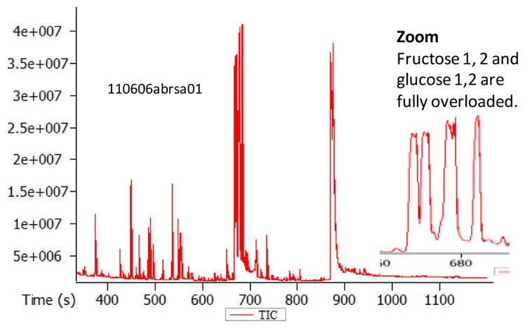
Example chromatogram for overloaded injection of a plant extract. If too much sample is injected, peak intensities exceed column and detector capacities. For such overloaded peaks, any quantitative readout is impossible, as shown here for fructose and glucose. Note that metabolites that bear keto- or aldehyde groups like these two sugars form two peaks due to the methoximation reaction.

The process of Quality Control checks and monitoring, and some suitable maintenance procedures to restore high quality data acquisitions, is given in Figure 6 as flow chart. It is important to recognize that this flow chart gives a non-exclusive list of specific examples, and typical remedies if quality controls fail. However, neither the Quality Control checks nor the maintenance procedures are comprehensive. There are many more possibilities how data acquisitions may fail, but these are relatively rare, from broken columns to failing septa, thermo sensors, or electronic parts. Note that several times, a suggested maintenance measure is to cut the column (10–15 cm). For this reason, we recommend using a 10 m empty guard column (without polysiloxane film) that can be cut many times without changing the relative distance between peaks (precisely because the empty guard column does not have a film, i.e. does not contribute to the separation of compounds). Many problems observed in GC-MS data acquisition quality are due to matrix effects, or contaminations that build up in liners and ultimately in the begin of the column.

Figure 6. Quality control flowchart overview for reference compound mixture and pooled samples.

Summarized overview of quality control steps and suggested remedies for QC failures. Poor quality in GC/MS based metabolomics can be attributed to the injection system in 80% of the cases. Refer to instrument maintenance manuals for proper GC/MS operation.

Basic Protocol 4: GC-MS data processing for metabolome analysis

Introduction

Data processing is under constant development in metabolome analysis. Due to the decades-long standardization efforts in GC-MS, data sets are much easier processed and more comparable than in LC-MS. Most importantly, the ionization/fragmentation spectra differ very little among instruments. Secondly, the concept of retention indices was introduced fifty years ago (Kovats, 1965), using a series of aliphatic alkanes as retention markers across chromatograms and then replacing absolute retention times (which vary by column lengths and column aging) by assigned retention indices (which are fixed in relation to the retention index marker compound anchors). The only difference to this concept that is used in the protocols here is to use fatty acid methyl esters (FAMEs) instead of aliphatic alkanes. In electron ionization, FAMEs yield characteristic fragment ions (such as m/z 74 and m/z 87) in addition to detectable molecular ions, whereas aliphatic alkanes fragment so rapidly that no molecular ions are detectable. For staff, as well as for computational routines, the correct identification of these retention marker ions is much more straightforward if such molecular ions and higher m/z fragments are present, which is not the case for alkanes. In order to avoid confusion, the Fiehnlib libraries (Kind et al, 2009) and BinBase (Fiehn et al, 2008) use arbitrarily assigned large retention index numbers instead of the Kovats system that multiplies the aliphatic carbon chain length by a factor of 100. In both retention index systems, all retention times are then converted to retention indices by linear or polynomial regressions.

Importantly, use of retention index systems has two main advantages:

1. alignment of detected peaks and their retention times between samples is not dependent any longer on the similarity of such samples, as is the case in data processing systems used in LC-MS metabolomics such as XCMS (Smith et al, 2006) or (the better performing) MZmine software programs (Katajamaa et al, 2006). Alignments in GC-MS only rely on the matrix of internal reference markers used, and in the Fiehn laboratory, over 130,000 GC-TOF MS samples have been processed in this way through the BinBase database system over the past 10 years. Data processing and data comparisons can therefore encompass largely different types of samples (e.g., blood and urine samples), in order to find compounds that might be present in both matrices.

2. detection and presence of unidentified metabolites is no longer tied to a specific sample or biological matrix. Instead, both identified compounds as well as novel, structurally unknown biomarkers can be stored in the same database (in this UNIT: the BinBase database). Similarly, libraries of known compounds that are collated in publicly available repositories such as the NIST14 library can be used for both retention time and mass spectral matching, because Kovats indices can be readily transformed into Fiehnlib retention indices by a single injection containing both Kovats alkane standards and Fiehnlib FAME reference markers. Hence, GC-MS enables a straightforward combination of targeted metabolomics (through MS and retention-based libraries of reference compounds) and untargeted metabolomics (through MS and retention-based databases of novel unknown markers).

Materials List

Software

(a) For Leco GC-TOF MS data sets

• ChromaTOF instrument peak finding and mass spectral deconvolution software, version 4.0 or higher

• BinBase database software (open source; https://code.google.com/p/binbase/) See publications for detailed software descriptions. (Skogerson et al, 2011)

(1) For Agilent GC-quadrupole MS data sets

• Automated mass spectral deconvolution and identification system (AMDIS) (from the National Institute of Standards and Technology (NIST))

• SpectConnect software (developed by Georgia Tech) (Styczynski et al, 2007)

Steps and Annotations

These steps are only given for Leco GC-TOF MS data processing as this is far more advanced than data processing for GC-quadrupole MS instruments. However, the concepts given below can be adapted through AMDIS and SpectConnect software also for quadrupole GC-MS data sets, but are not presented in this UNIT.

(1) Raw data preprocessing

Pre-process raw data files directly after data acquisition and store result files as ChromaTOF-specific *.peg files, as generic *.txt result files and additionally as generic ANDI MS *.cdf files. Use ChromaTOF version 4.2 or higher for data preprocessing without smoothing, 3 s peak width, baseline subtraction just above the noise level, and automatic mass spectral deconvolution and peak detection at signal/noise levels of 5:1 throughout the chromatogram. Report apex masses for use in the BinBase algorithm. Export result *.txt files in ChromaTOF to a data server with absolute spectra intensities. Process results data further by a filtering algorithm implemented in the metabolomics BinBase database.

(2) Data validation, alignment and filtering

Use the BinBase algorithm (rtx5) with the following settings: validity of chromatogram (<10 peaks with intensity >10^7 counts s-1), unbiased retention index marker detection (MS similarity>800, validity of intensity range for high m/z marker ions), and retention index calculation by 5th order polynomial regression.

Users cannot change parameter settings in BinBase unless users are trained in Java programming. For clarity, the BinBase algorithm is outlined here: In BinBase, mass spectra are cut to 5% base peak abundance and matched to database entries from most to least abundant spectra using the following matching filters: retention index window ±2,000 units (equivalent to about ±2 s retention time), validation of unique ions and apex masses (unique ion must be included in apexing masses (all ions that have the highest intensity at the peak apex retention time of the unique ion) and present at >3% of base peak abundance), and mass spectrum similarity must fit criteria dependent on peak purity and signal/noise ratios and a final isomer filter. Failed spectra are automatically entered as new database entries if s/n >25, purity <0.1 and presence in the biological study design class was >80%. Quantification is reported as peak height using the unique ion as default, unless a different quantification ion is manually set in the BinBase administration software BinView. A subsequent post-processing module is employed to automatically replace missing values from the *.cdf files. Replaced values are labeled as ‘low confidence’ by color coding, and for each metabolite, the number of high-confidence peak detections is recorded as well as the ratio of the average height of replaced values to high-confidence peak detections.

Surprisingly, results from such types of data alignments and filtering are very similar to reports using AMDIS and SpectConnect software. Indeed, about half of all spectra detected in ChromaTOF/BinBase or in AMDIS/SpectConnect are too low abundant and/or too noisy to be compared across samples and studies. In BinBase, known chemical artifacts such as polysiloxanes, phthalates or derivatization reagent by-products are automatically recognized and are not exported to biological results data sheets.

(3) Manual data curation

An example of such a ‘raw data’ results is given in Figure 7. Report the actual intensity data are as peak heights (as shown) or peak areas, but specify the quantification ion (m/z value) and the specific retention index. Giving peak heights instead of peak areas is recommended, because peak heights are more precise for low abundant metabolites than peak areas, due to the larger influence of baseline determinations on areas compared to peak heights. Also, overlapping (co-eluting) ions or peaks are harder to deconvolute in terms of precise determinations of peak areas than peak heights. Call such data files ‘raw results data’ in comparison to the raw data file produced during data acquisition.

Figure 7. Example sheet to report raw result data.

Results may need to be further curated before final submission and input for statistics and bioinformatics research. Given here is a result sheet from a Leco GC-TOF MS instrument with Fiehnlab BinBase database annotations (Fiehn et al, 2005). Rows: The compound annotation must include the chemical name, at least one unique database identifier (here: structural InChI key (Heller & McNaught, 2009)), metadata on which the compound annotation is based (here: retention index, quantification mass, BinBase identifier and full mass spectrum, encoded as string), and bioinformatics keys such as KEGG (Kanehisa & Goto, 2000)and PubChem (Bolton et al, 2008). For curation, this raw results sheet also lists how often each peak was confidently identified in the experiment (‘count’), how abundant these peaks were on average (‘det’), and if these were not confidently detected, how abundant the replaced values were (from raw chromatograms), ‘repl’. Values that have been replaced are marked in orange color. The data curator decides which peaks would be deleted, e.g. xylonolactone that was only positively detected in 1/50 samples. If two or more peaks annotate the same unique metabolite, these rows are added up (e.g. valine + valine 1TMS). Columns: For each sample, the raw file identifier must be given in addition to all available biological information such as species, organ and treatment. Here, the columns also denote the LIMS identifiers (mx), the count of confidently identified peaks (count), the sum peak height of the internal standards (fTIC) and the sum peak height of all structurally annotated compounds (mTIC) as sum parameter for normalizations.

Do not use chemical names as unique compound identifier (e.g., “alanine”); instead, use external database identifiers, such as InChI key, PubChem ID and KEGG ID for unambiguous structural annotation of the compound. Specifically, the ‘InChI key’ identifier is most suitable to detail the unique chemical structure as it is defined and supported by both IUPAC and NIST, and because it is automatically scanned in Pubmed and hence, searchable in Pubmed or Google queries. However, for communication with biologists, using clear biochemical names is advantageous (here: The ‘BinBase name’ denotes the name of identified metabolites.) If a compound is unknown, use a clear identifier as name, for example, a combination of retention index and quantification ion, or a database identifier (here: BinBase id). Use a ‘retention index’ column to detail the target retention index in the BinBase database system. Use a ‘quant mz’ column to detail the m/z value that was used to quantify the peak height of a BinBase entry. Use an ‘identifier column’ to denote the unique identifier for the GCTOF MS platform, in case you employ a coherent database system (using unambiguous identifiers with unique metadata for each entry and a memory coherence protocol to ensure that all links to these entries are updated automatically if changes are made). Such unique identifiers are critically important if you want to report ‘unknowns’ along with identified metabolites. If you do not operate a coherent database system, at least report unknowns by retention index, quantification mass and deconvoluted mass spectrum. Report a ‘mass spec’ column to detail the complete mass spectrum of the metabolite given as m/z: intensity values, separated by spaces; otherwise, you could give here the database identifier of a mass spectral entry (e.g., NIST) if you have used such mass spectral repository for compound identification. Add an additional ‘internal standard’ column to clarify, if a specific chemical has been added into the extraction solvent as internal standard. These internal standards may serve for quality control purposes or for quantification normalizations.

In a manual method, curate the raw results file as follows : Use the 10% quantification report table that is produced for all database entries that are positively detected in more than 10% of the samples of a study design class for unidentified metabolites. Then, delete compounds that have not been positively detected (red color coding, Fig. 7) by thresholds that fit your biological design. For example, some compounds may only be detected in a specific biological situation, and hence would be undetected (red color coding) in other study design classes. Calculate the total number of positive peak detections over the study (column ‘count’), but also calculate the average peak height of the positively detected peaks (column ‘det’), the peak heights of replaced values (column ‘repl’) and the ratio of these two values. If you use the BinBase database systems, such values will be automatically calculated for you. Delete metabolite rows by limiting the maximum ‘replaced’ value that fits your expectations. These ‘replaced’ values may occasionally be higher than the high-quality detected peaks. For example, see zC12 FAME internal standard with a ratio repl/det of 1.6, indicating that some true C12FAME peaks were not correctly deconvoluted by the ChromaTOF software and hence, not positively identified in the BinBase DB system. However, never use chromatographic peaks (metabolite rows) that are reported at ratios >3, and always delete metabolite rows that have an absolute count of less than six truly detected peaks. Next, combine metabolite rows that have two or more individual peaks detected in GC-MS reports, such as xylose2 and xylose (due to the syn/anti-forms during methoximation) or valine.1TMS and valine.2TMS (due to the incomplete derivatization of N-TMS groups as mentioned above). BinBase does not provide these peak combinations in an automated way in order to force users to perform a careful investigation of result sheets themselves. Next, introduce a row “fTIC” and calculate in this row the sum of all FAME internal standards, to provide an overall quality control measure. Use fTIC values for normalizations across machine drifts as necessary. Introduce a row “mTIC” and calculate in this row the sum of all positively identified metabolites (here: compounds with BinBase names). This row gives an overall measure of the total metabolome detected in a given sample which can be used for semi-quantitative normalizations as long as the mTIC values do not show a significant difference between classes in the study design, based on t-test statistics at p <0.05.

Tailor row sample metadata to specific biological and data file information, but make sure to comprise always at least the following metadata: Data file names need to be identical to file names submitted to the NIH Metabolomics database, www.metabolomicsworkbench.org. Best practice is to denote metadata information in the file name itself, for example, the date when the file sequence was generated by YYMMDD, the particular GC-MS instrument used for data acquisition’ (here: instrument b), the person who operated the machine (here: ct for laboratory assistant Carol Tran), what type of injection the data include (here: ‘sa’ for sample, instead of ‘qc’ for a quality control or ‘bl’ for a blank sample), followed by the injection sequence number. If you use a laboratory information management system (LIMS), add a row that specifies the according LIMS identifier (here: miniX class ID and miniX sample information as mx data). Include rows for comments, species, organ, and treatment information to denote the specifics of a biological experiment.

(b) Final data reporting

Finally, report normalized metabolomic data including metadata, see example from the same study in Figure 8. As you can see, xylose and xylonolactone, for example, have been deleted, and valine is now given as single (combined) value. Use such curated reports in all communications with collaborators in biology, bioinformatics, statistics or medicine, as these curated data sets comprise all information needed for biochemical and statistical analyses, uploads of data sets to community databases or as supplementary information for journal publications.

Figure 8. Example sheet to report final result data.

Before final result submission, curation columns and curation rows are deleted (compare to figure 6), reporting the most reliably detected compounds. There is no consensus yet in the metabolomics community on thresholds to be used for compound annotations, or curation of results. Recommended is to report peaks that are confidently detected in at least 80% of the samples of at least one study design group (e.g. the R1 mouse embryonic stem cells used in the example displayed here).

Raw results data need to be normalized to reduce the impact of between-series drifts of instrument sensitivity, caused by machine maintenance, aging and tuning parameters. There are many different types of normalizations in the scientific literature, and there is no general consensus. Try the following schema:

1. Perform a t-test statistics test if the mTIC (the sum of all identified metabolites) differ between the different study design classes in your study.

2. If the mTIC is not significantly different at p<0.05 between your classes, perform a variant of a ‘vector normalization’, normalize your data sample-by-sample to the total average mTIC.

Following equation is then used for normalizations for metabolite i of sample j:

$${\text{metabolite}}_{ij,\text{normalized}}={\text{metabolite}}_{ij,\text{raw}}/{\text{mTIC}}_j\ast {\text{mTIC}}_{\text{average}}$$

Call this worksheet ‘norm mTIC’. Data are ‘relative semi-quantifications’, meaning they are normalized peak heights.

Note that such average mTIC will be different between series of analyses that are weeks or months apart, due to differences in machine sensitivity, tuning, maintenance status and other parameters. If you want to compare across batches of studies that are analyzed months apart, perform additional normalizations. Use identical samples (‘QC samples’) for this purpose that must be analyzed multiple times in all series of data acquisitions.

If you want to test for drifts within a batch of e.g. 300 samples, use the following statistical analysis: (a) compute univariate statistics for mTIC values in batches within-series and between-series of data injections, using time/date stamps to find potential breaks during which machine downtime may have occurred. If there are no mTIC differences between such time/date stamp batches, calculate an overall mTIC covering all samples. (b) compute multivariate PCA plots for the study, marking the potentially different samples of individual time/date stamp batches using different colors. If there is no apparent separation between PCA clusters of different colors, there is no large between-series effect and these PCA clusters can be treated as indistinguishable. If there is suspicion of hidden features that might be masked by overall variance analysis in PCA, supervised statistics by Partial Least Square regression models can unravel such between-series differences.

In case you identify different clusters (i.e. series of undistinguishable QC samples) within a set of, for example,300 samples, you need to develop correction factor models that correct for differences between those QC samples. Subsequently, these correction factors would need to be applied to the actual analytical samples to remove overt quantification differences that are not related to biological causes but solely due to analytical errors.

Such correction factor models can be computed in different ways, e.g. by unit-variance mean centering or by calculating simple offset vectors for each individual metabolite. However, in any case, such correction models can only be developed if a sufficient number of QC samples have been included in the analytical sequences.

For that reason, use a suitable QC sample for every 11th injection. Such QC samples need to be as similar to the actual biological specimen as possible(e.g., generated by pool samples during extractions) or by obtaining typical community standard samples (e.g., the NIST standard blood plasma, or commercial serum or plasma samples as needed).

If appropriate internal standards are used for absolute quantifications, the following equation could be used for peak height normalizations for metabolite i of sample j and internal standard k

$${\text{metabolite}}_{ij,\text{normalized}}={\text{metabolite}}_{ij,\text{raw}}/{\text{istd}}_k\ast \text{concentration}{\text{istd}}_k$$

However, there are few universal or class-specific internal standards in GC-MS based analysis, because within each chemical class, metabolites may have drastically different calibration curves (sensitivity or ‘response’) based on a combination of injection, volatilization and stability and ionization response properties. As surrogate, you can use external calibration standards for specific (important) metabolites which, however, cannot be applied for unidentified compounds and which of course would not account for recovery during extraction procedures.

Reagents and Solutions

Equipment

• microtube centrifuge, e.g. Labconco Centrivap with large phenol-free lid seal and built-in vacuum delay to prevent bumping by allowing the rotor to achieve speed before applying vacuum.

• calibrated micropipettes 1–200 μl and 100–1000 μl

• polypropylene microtubes 1.5 ml, uncolored (colored microtubes may leak contaminant chemicals into the mixture). For example, 1.5 mL Eppendorf PCR tubes with hinged safe-locks that prevent accidental lid opening are well suited.

• mini vortexer

• precision balance with accuracy ± 0.1mg

• volumetric flasks

• sonicator

Chemicals

• methanol LCMS grade quality

• isopropanol, LCMS grade quality

• ultrapure water with <18 mΩ residual conductivity

• nitrogen gas line with glass pipette tip

Recipe for Quality Control mix of external reference standards

1. Prepare 500 ml solution A as a mixture of H₂O: methanol : isopropyl alcohol (1:2.5:1, v/v/v).

   Purge solution with nitrogen gas for 5 minutes to remove dissolved oxygen, for example using a pasteur pipet attached to a polypropylene line connected to a nitrogen gas tank.

2. Weigh standards into a glass vial according to Table 1 to 0.1 mg accuracy. Dissolve standards in (1 ml to 1.5 ml) appropriate solvents as listed in Table 1 in 2 ml Eppendorf tubes. Vortex mix for 10 s.

   Dissolve aspartic acid, glutamic acid, and adenosine to 1 mg/mL (20 mL, 10 mL, and 10 mL respectively) in solution A. These three compounds are difficult to dissolve at 10 mg/mL. For dissolving aspartic, add 5 uL at a time of 0.2 M NaOH after dissolving to 1 mg/mL.

3. Add approximately 25 mL of solution A to a 250 mL volumetric flask with glass stopper.

4. Transfer all the standard solutions quantitatively to 250 mL volumetric flask and adjust the volume by filling 250 mL volumetric flask with solution A to the calibration mark.

5. Mix the QC mix for about 30 minutes (or more) to completely dissolve all compounds. This is the stock solution. Concentration of the various compounds in the stock solution is 40 μg/mL. This solution is stored in a refrigerator. The solution has a shelf life of 2 months.

6. To make a working Quality Control mix: Dilute 2.5 mL stock solution to 10 mL with solution A to obtain a working concentration of 10 μg/mL. This standard solution is kept in the refrigerator.

7. Six-point QC mix samples are pipetted from working QC mix into 2 ml Eppendorf vials.

   • QC6: 50 μL aliquot → 500 ng/compound in vial

   • QC5: 25 μL aliquot → 250 ng/compound in vial

   • QC4: 10 μL aliquot → 100 ng/compound in vial

   • QC3: 5 μL aliquot → 50 ng/compound in vial

   • QC2: 2.5 μL aliquot → 25 ng/compound in vial

   • QC1: 1.0 μL aliquot → 10 ng/compound in vial

     All aliquots are taken when the solutions are at room temperature and standard solutions should be inspected before aliquots are taken so there is no precipitation.

8. QC mixes are dried down, derivatized and analyzed according to Basic Protocol 1.

   If 100 ul reagent volumes are used for derivatization, and 1 ul is injected (for GC-quadrupole MS), then QC4 would represent ca. 1 ng injected onto the column per compound

9. Six point calibration standards are visually evaluated before and after each GC- MS analysis (see Figures 2–4).

   As these QC mixes represent external calibration curves, they can be used for absolute quantification of metabolites in biological samples using regression curves in Microsoft Excel, but only for those compounds included in the QC mixes.

As example, compounds of this Quality Control mixture are then detected by GC-MS using the quantification ions, retention times and methoximation/trimethylsilylation derivatives as given in Table 2, corresponding to examples given in Figures 2–4.

Please note that all retention times are given as examples and need to be referred to the FAME QC mix to obtain retention indices. A retention index is defined system of numbers that spans consistent intervals between each retention index marker compound. The classic Retention Index is the Kovats index for alkanes, with C8 alkane defined as Retention Index number 800, C9 alkane defined as number 900 and so on. In order not to confuse scientists, the Fiehn retention index uses much larger numbers, see Table 3. Experimental retention times in each set of chromatograms need to be converted to absolute retention indices using regression curves in table calculation software, e.g. Microsoft Excel.

Table 3.

Details to prepare and use the FAME mixture as internal standards.

Chemical	Fiehn retention index value	Kovats retention index value	amount (mg)	concentration (mg/mL)
Methyl caprylate/octanoate (C08)	262320	1083	20	0.8
Methyl pelargonate/nonanoate (C09)	323120	1183	20	0.8
Methyl caprate/decanoate (C10)	381020	1282	20	0.8
Methyl laurate/dodecanoate (C12)	487220	1481	20	0.8
Methyl myristate/tetradecanoate (C14)	582620	1680	20	0.8
Methyl palmitate/hexadecanoate (C16)	668720	1878	20	0.8
Methyl stearate/octadecanoate (C18)	747420	2077	10	0.4
Methyl arachidate/icosanoate (C20)	819620	2276	10	0.4
Methyl behenate/docosanoate (C22)	886620	2475	10	0.4
Methyl tetracosanoate (C24)	948820	2674	10	0.4
Methyl hexacosanoate (C26)	1006900	2872	10	0.4
Methyl octacosanoate (C28)	1061700	3071	10	0.4
Methyl triacontanoate (C30)	1113100	3270	10	0.4

Preparation of a mixture of internal markers of fatty acid methyl esters (FAMEs)

• Use the amounts given in Table 3 of each FAME into separate 1.5 ml glass vials.

• Add 1 ml chloroform to each glass vial and vortex to mix.

• Combine the contents of all 13 vials into a 25 ml volumetric glass stoppered flask.

• Add additional chloroform to bring final volume to 25 ml.

• Mix using a stir plate/stir bar.

• Transfer contents to an amber bottle and label as FAME internal marker solution. Solution is usable for one year. Store in fridge. Use Fiehn retention index values or corresponding Kovats retention indices to report all peaks as normalized retention index.

Preparation of a reagent blank

1. Prepare 20 mg/mL Methoxyamine hydrochloride [MeOX] solution in pyridine.

2. Vortex MeOX solution and sonicate at 60 °C for 15 min to dissolve.

3. Add 10 μL of MeOX solution to an autosampler vial.

4. Add 91 μL of MSTFA + FAME mixture to the autosampler vial. Cap immediately.

5. Submit to GC-MS data acquisition.

Preparation of a method blank

Use all steps and procedures as outlined in Basic Protocol 1 except for using an actual sample (blood, urine, cells or tissues). Instead, use an empty sample tube that is subjected in an identical way as all samples, including shaking, solvents and heating.

Commentary

Background Information

Gas chromatography-mass spectrometry has one huge advantage over other methods in metabolomics: it works from Day One. Many pathway intermediates from glycolysis, pentose phosphate pathway, TCA cycle (Krebs Cycle) and other major pathways in primary metabolism are well covered. Gas chromatographic resolution is superb, in comparison to liquid chromatography, with peak widths of roughly 2–3 seconds, when using the methods detailed above. Of course, GC-MS metabolome profiling has also its limitations: thermolabile compounds cannot be analyzed intact, and indeed, some detected unknown compounds may in fact be artifacts that are formed during the hot injection and separation. In general, diphosphates, as well as bis- or trisphosphates (e.g., NADH or ATP) cannot be analyzed by GC-MS, while monophosphates (e.g., glucose-6-phosphate or phosphoenolpyruvate) are detected very sensitively as trimethylsilyl-derivatives. Indeed, GC-MS is best suited for sugars and hydroxyl acids, which are much harder, if not impossible, to separate in LC-MS based metabolomics screens. A second disadvantage of GC-MS based metabolomics is that biogenic amines, including amino acids, show severe matrix effects and are hard to control with respect to relative and absolute peak heights of underivatized and derivatized trimethylsilylation forms of the primary amino group. However, when the injector, liner, syringe and first 15 cm of the column are kept meticulously clean, and when Quality Control samples are routinely monitored to keep the N-derivatives intact, then full primary metabolism profiling is best achieved by GC-MS. On the other hand, if absolute quantification of amino acids is critical, GC-MS still offers other options such as the use of the far more stable tert.butyldimethyl-derivatives, using tert.butyldimethylsilyl-trifluoroacetamide (MTBSTFA). Hence, for profiling primary metabolism, GC-MS remains the Gold Standard (i.e., a standard to which all other available methods are compared), whereas LC-MS is the method of choice for secondary (specific) large metabolites such as flavonoids or glucosinolates, as well as for large and complex lipids. These techniques are truly complementary and should both be employed to obtain full coverage of metabolomics data in biological studies.

Critical Parameters

Critical parameters have been extensively discussed in Support Protocol 1 on “quality controls”.

Troubleshooting

Ensure that the GC-MS system is fully operational. Start with system suitability tests as given in your instrument’s manuals, especially for tuning the instrument. Tuning parameters and tuning results will readily indicate if the mass spectrometer portion of your GC-MS system is in control, yielding high quality, sensitive measurements. Afterwards, test your GC-MS system by injecting very simple mixtures, such as the FAME mixture outlined in Table 3. If FAME peaks show peak distortions (see Fig 2a, e.g., for early eluting C08 methyl octanoic acid), or if FAME peaks show injector discrimination (e.g., for high boiling C30 methyl triacontanoic acid), then solve these problems before testing any metabolomics sample. At least 80% of all problems you may encounter are due to the “injector” (i.e., gas flows, gas leaks, pressure control, loose fittings and liner incompatibilities. Ensure that you have all necessary parts ready to maintain your instrument, including gas leak detectors, nuts, ferrules, spare columns, filaments and other consumables. Do not shy away from changing liners or other consumable parts! Good maintenance means that consumables and spare parts are exchanged before problems arise, not afterwards. You need to avoid detecting quality control problems when you analyze large sets of metabolomics samples: at that time, all data have been acquired, and you cannot change anything anymore to get high quality data. Normalization is not a means to fix problems that happened during data acquisition.

Most mass spectrometers (such as quadrupole or TOF MS analyzers) are so well engineered that problems may only arise after intensive usage. However, there are certainly differences between manufacturers with respect to robustness of instruments. One of the general problems in massspectrometry-based metabolomics is that the instruments get into physical contact with the sample, unlike to NMR, where the sample is contained in a spinning tube inside the magnetic field. Hence, contaminations are unavoidable. In GC-MS, most of the contamination (or matrix) stays in the liner (i.e., the injector interface) and the first 15 cm of the column. However, after long use, matrix depositions are also build-up at the ion source. Depending on the physics of the ion source used, frequent cleaning may be necessary, potentially once every 2 weeks. Consider the time required for ion source cleaning a real expense because staff hours are needed, and because the instrument’s downtime reduces overall productivity. Compare downtime statistics between instrument types and manufacturers to make the best investment decision.

The ion source in GC-MS also contains the filaments that produce the high-energy electrons. Such filaments may need to be replaced, somewhere between once a year and once every two months, but it may also happen that you need to change filaments several times within one month, if you have nasty matrix problems or technical issues. Lastly, TOF mass spectrometers usually use multichannel plates as detectors (unlike quadrupole MS instruments). Such multichannel plates wear out and may need to be replaced yearly to maybe once every two years. However, if you maintain your instrument condition well, you can easily use a GC-MS for 10 years or longer.

Apart from the instruments that are recommended to be used in this UNIT, there are also modern variants, including accurate mass TOF and QTOF MS analyzers. In general, such accurate mass GC-MS instruments show less robustness and need more maintenance efforts than nominal-mass quadrupole or nominal-mass TOF MS instruments, used in this UNIT. Do not only rely on such accurate mass GC-MS instruments, but combine the best of both worlds, the robustness of nominal-mass GC-MS instruments for high throughput profiling with the additional benefits of high resolution accurate mass GC-MS instruments that can give you capacity to identify unknowns or to verify the purity of specific peaks. Other instruments such as two-dimensional chromatography in GCxGC-MS or enhanced selectivity in GC-MS/MS are also available and may serve special purposes. In principal, sample preparation and derivatization protocols are identical or very similar to the ones outlined in Basic Protocol 1. However, data acquisition and data processing may differ tremendously, requiring a significant amount of time in method development. Hence, start with simple procedures as given in this UNIT before you try using more advanced methods.

Anticipated Results

Depending on the sample and the instrument used, GC-MS based metabolomics regularly identifies 100–200 primary metabolites in a given biological study, as well as detects 150–350 additional unidentified metabolites. As there is almost no matrix effect during the ionization process, unlike to LC-MS protocols, you can use external standardsand mixture of reference compounds (see Basic Protocol 3), for calculating absolute concentrations. An example for such external calibration mix was given in the Recipe for Quality Control solutions of external reference standards. However, such external standards cannot be used to control for effects during sample harvesting, enzyme quenching (stopping enzymatic activity), storage, extraction, cleanup (removal of interfering matrix components, e.g. triglycerides) and derivatizations. These effects are the largest causes of analytical errors, both systematic errors and random errors. Unfortunately, there are no internal standards available that could correct for such sample preparation errors for all primary metabolites, because the response factors (‘sensitivity’) for primary metabolites in GC-MS are different for all compounds. You cannot use (e.g., stable isotope-labeled glycine) as internal standard for all amino acids, as asparagine or serine will show drastically different calibration curves (and losses). Therefore, use a two-phase design in GC-MS based metabolomics: in the discovery phase I, use semi-quantitative profiling as used in this UNIT. After statistical evaluations and biological interpretations (see Basic Protocol 4), repeat the study with few, very specific internal standards in a validation phase II, in which accurate and absolute molar quantifications can be achieved.

Time Considerations

Extractions and derivatizations can be easily performed for 40 samples per day by a single staff person. Using six reference mixture quality control samples, four biological pool quality control samples and 4 blank quality control samples, a total of 58 injections per day or up to 200 biological samples per week can be acquired, if GC-MS run times are kept at 20 minutes per sample as given above. If no technical or matrix problems occur, a well-maintained GC-MS instrument can acquire up to 6,000 samples per year, given downtime for planned maintenance, vacation and other disruptions of workflows. However, this high throughput sample acquisition is only possible for very well trained and highly experienced staff, and only if there are no major technical problems with the equipment. Please be aware that the first problem you encounter may be a problem that is neither easily recognized nor quickly resolved. Fixing problems may therefore take 50% of the time, especially when a laboratory implements new procedures that have not used before. Use help given in online tutorials (such as by the ChromAcademy, www.chromacademy.com), experts in user groups like LinkedIn, expertise given in magazines like LC-GC, and use personal contacts and professional networks to discuss technical problems and solutions.

More severe are time considerations for untargeted metabolomics and compound identification. Experience helps, but eventually, researchers need to plan for sufficient time analyzing and scrutinizing raw data sets, from chromatograms and mass spectra to result data sets given above. When starting a new project, expect using 10-times as much time in front of a computer screen than you have spent in the laboratory. It is very easy and quick to acquire data. It is harder and slower to acquire high quality data. But it is very cumbersome and slow to correctly process and interpret metabolomics data, be these GC-MS based or LC-MS based data.

Literature Cited

- Aksenov AA, Pasamontes A, Peirano DJ, Zhao W, Dandekar AM, Fiehn O, Ehsani R, Davis CE. Detection of Huanglongbing disease using differential mobility spectrometry. Analytical chemistry. 2014;86:2481–2488. doi: 10.1021/ac403469y. [DOI] [PubMed] [Google Scholar]
- Anggard E, Sedvall G. Gas chromatography of catecholamine metabolites using electron capture detection and mass spectrometry. Analytical chemistry. 1969;41:1250–1256. doi: 10.1021/ac60279a042. [DOI] [PubMed] [Google Scholar]
- Babushok VI, Linstrom PJ, Reed JJ, Zenkevich IG, Brown RL, Mallard WG, Stein SE. Development of a database of gas chromatographic retention properties of organic compounds. Journal of Chromatography A. 2007;1157:414–421. doi: 10.1016/j.chroma.2007.05.044. [DOI] [PubMed] [Google Scholar]
- Bolton EE, Wang Y, Thiessen PA, Bryant SH. PubChem: integrated platform of small molecules and biological activities. Annual reports in computational chemistry. 2008;4:217–241. [Google Scholar]
- Brooks CJW, Horning EC, Young JS. Characterization of sterols by gas chromatography-mass spectrometry of the trimethylsilyl ethers. Lipids. 1968;3:391–402. doi: 10.1007/BF02531277. [DOI] [PubMed] [Google Scholar]
- Buszewski B, Ligor T, Jezierski T, Wenda-Piesik A, Walczak M, Rudnicka J. Identification of volatile lung cancer markers by gas chromatography–mass spectrometry: comparison with discrimination by canines. Analytical and bioanalytical chemistry. 2012;404:141–146. doi: 10.1007/s00216-012-6102-8. [DOI] [PMC free article] [PubMed] [Google Scholar]
- Coward RF, Smith P. The gas chromatography of aromatic acids as their trimethylsilyl derivatives, including applications to urine analysis. Journal of Chromatography A. 1969;45:230–243. doi: 10.1016/s0021-9673(01)86205-1. [DOI] [PubMed] [Google Scholar]
- DeJongh DC, Radford T, Hribar JD, Hanessian S, Bieber M, Dawson G, Sweeley CC. Analysis of trimethylsilyl derivatives of carbohydrates by gas chromatography and mass spectrometry. Journal of the American Chemical Society. 1969;91:1728–1740. [Google Scholar]
- Dixon E, Clubb C, Pittman S, Ammann L, Rasheed Z, Kazmi N, Keshavarzian A, Gillevet P, Rangwala H, Couch RD. Solid-phase microextraction and the human fecal VOC metabolome. PloS one. 2011;6:e18471. doi: 10.1371/journal.pone.0018471. [DOI] [PMC free article] [PubMed] [Google Scholar]
- Fiehn O. Metabolomics–the link between genotypes and phenotypes. Plant molecular biology. 2002;48:155–171. [PubMed] [Google Scholar]
- Fiehn O, Garvey WT, Newman JW, Lok KH, Hoppel CL, Adams SH. Plasma metabolomic profiles reflective of glucose homeostasis in non-diabetic and type 2 diabetic obese African-American women. PLoS One. 2010;5:e15234. doi: 10.1371/journal.pone.0015234. [DOI] [PMC free article] [PubMed] [Google Scholar]
- Fiehn O, Kind T. Metabolomics. Springer; 2007. Metabolite profiling in blood plasma; pp. 3–17. [DOI] [PubMed] [Google Scholar]
- Fiehn O, Kopka J, Dörmann P, Altmann T, Trethewey RN, Willmitzer L. Metabolite profiling for plant functional genomics. Nature biotechnology. 2000a;18:1157–1161. doi: 10.1038/81137. [DOI] [PubMed] [Google Scholar]
- Fiehn O, Kopka J, Trethewey RN, Willmitzer L. Identification of uncommon plant metabolites based on calculation of elemental compositions using gas chromatography and quadrupole mass spectrometry. Analytical chemistry. 2000b;72:3573–3580. doi: 10.1021/ac991142i. [DOI] [PubMed] [Google Scholar]
- Fiehn O, Wohlgemuth G, Scholz M. Setup and annotation of metabolomic experiments by integrating biological and mass spectrometric metadata. Data integration in the life sciences. 2005:224–239. [Google Scholar]
- Fiehn O, Wohlgemuth G, Scholz M, Kind T, Lee DY, Lu Y, Moon S, Nikolau B. Quality control for plant metabolomics: reporting MSI-compliant studies. The Plant Journal. 2008;53:691–704. doi: 10.1111/j.1365-313X.2007.03387.x. [DOI] [PubMed] [Google Scholar]
- Gao X, Pujos-Guillot E, Martin J-F, Galan P, Juste C, Jia W, Sebedio J-L. Metabolite analysis of human fecal water by gas chromatography/mass spectrometry with ethyl chloroformate derivatization. Analytical biochemistry. 2009;393:163–175. doi: 10.1016/j.ab.2009.06.036. [DOI] [PubMed] [Google Scholar]
- Gelpi E, Koenig WA, Gibert J, Oro J. Combined gas chromatography-mass spectrometry of amino acid derivatives. Journal of Chromatographic Science. 1969;7:604–613. [Google Scholar]
- Gréen K. Gas chromatography—Mass spectrometry of O-methyloxime derivatives of prostaglandins. Chemistry and physics of lipids. 1969;3:254–272. doi: 10.1016/0009-3084(69)90017-6. [DOI] [PubMed] [Google Scholar]
- Halket JM, Przyborowska A, Stein SE, Mallard WG, Down S, Chalmers RA. Deconvolution gas chromatography/mass spectrometry of urinary organic acids–potential for pattern recognition and automated identification of metabolic disorders. Rapid communications in mass spectrometry. 1999;13:279–284. doi: 10.1002/(SICI)1097-0231(19990228)13:4<279::AID-RCM478>3.0.CO;2-I. [DOI] [PubMed] [Google Scholar]
- Heller SR, McNaught AD. The IUPAC international chemical identifier (InChI) Chemistry International. 2009;31:7. doi: 10.1186/s13321-015-0068-4. [DOI] [PMC free article] [PubMed] [Google Scholar]
- Hopfgartner G, Tonoli D, Varesio E. High-resolution mass spectrometry for integrated qualitative and quantitative analysis of pharmaceuticals in biological matrices. Analytical and bioanalytical chemistry. 2012;402:2587–2596. doi: 10.1007/s00216-011-5641-8. [DOI] [PubMed] [Google Scholar]
- Horai H, Arita M, Kanaya S, Nihei Y, Ikeda T, Suwa K, Ojima Y, Tanaka K, Tanaka S, Aoshima K. MassBank: a public repository for sharing mass spectral data for life sciences. Journal of mass spectrometry. 2010;45:703–714. doi: 10.1002/jms.1777. [DOI] [PubMed] [Google Scholar]
- Kanehisa M, Goto S. KEGG: kyoto encyclopedia of genes and genomes. Nucleic acids research. 2000;28:27–30. doi: 10.1093/nar/28.1.27. [DOI] [PMC free article] [PubMed] [Google Scholar]
- Katajamaa M, Miettinen J, Orešič M. MZmine: toolbox for processing and visualization of mass spectrometry based molecular profile data. Bioinformatics. 2006;22:634–636. doi: 10.1093/bioinformatics/btk039. [DOI] [PubMed] [Google Scholar]
- Kind T, Wohlgemuth G, Lee DY, Lu Y, Palazoglu M, Shahbaz S, Fiehn O. FiehnLib: mass spectral and retention index libraries for metabolomics based on quadrupole and time-of-flight gas chromatography/mass spectrometry. Analytical Chemistry. 2009;81:10038–10048. doi: 10.1021/ac9019522. [DOI] [PMC free article] [PubMed] [Google Scholar]
- Kopka J, Schauer N, Krueger S, Birkemeyer C, Usadel B, Bergmüller E, Dörmann P, Weckwerth W, Gibon Y, Stitt M. GMD@ CSB. DB: the Golm metabolome database. Bioinformatics. 2005;21:1635–1638. doi: 10.1093/bioinformatics/bti236. [DOI] [PubMed] [Google Scholar]
- Kovats ES. Gas chromatographic characterization of organic substances in the retention index system. Adv Chromatogr. 1965;1:229–247. [Google Scholar]
- Kuksis A, Prioreschi P. Isolation of Krebs cycle acids from tissues for gas chromatography. Analytical biochemistry. 1967;19:468–480. doi: 10.1016/0003-2697(67)90238-2. [DOI] [PubMed] [Google Scholar]
- Kumari S, Stevens D, Kind T, Denkert C, Fiehn O. Applying in-silico retention index and mass spectra matching for identification of unknown metabolites in accurate mass GC-TOF mass spectrometry. Analytical chemistry. 2011;83:5895–5902. doi: 10.1021/ac2006137. [DOI] [PMC free article] [PubMed] [Google Scholar]
- Laine RA, Sweeley CC. Analysis of trimethylsilyl< i> O</i>-methyloximes of carbohydrates by combined gas-liquid chromatography-mass spectrometry. Analytical biochemistry. 1971;43:533–538. doi: 10.1016/0003-2697(71)90284-3. [DOI] [PubMed] [Google Scholar]
- Lee DY, Park J-J, Barupal DK, Fiehn O. System response of metabolic networks in Chlamydomonas reinhardtii to total available ammonium. Molecular & Cellular Proteomics. 2012;11:973–988. doi: 10.1074/mcp.M111.016733. [DOI] [PMC free article] [PubMed] [Google Scholar]
- Lu H, Liang Y, Dunn WB, Shen H, Kell DB. Comparative evaluation of software for deconvolution of metabolomics data based on GC-TOF-MS. TrAC Trends in Analytical Chemistry. 2008;27:215–227. [Google Scholar]
- Ma Y, Kind T, Yang D, Leon C, Fiehn O. MS2Analyzer: A Software for Small Molecule Substructure Annotations from Accurate Tandem Mass Spectra. Analytical chemistry. 2014;86:10724–10731. doi: 10.1021/ac502818e. [DOI] [PMC free article] [PubMed] [Google Scholar]
- Matyash V, Liebisch G, Kurzchalia TV, Shevchenko A, Schwudke D. Lipid extraction by methyl-tert-butyl ether for high-throughput lipidomics. Journal of lipid research. 2008;49:1137–1146. doi: 10.1194/jlr.D700041-JLR200. [DOI] [PMC free article] [PubMed] [Google Scholar]
- McLafferty FW, Hertel RH, Villwock RD. Probability based matching of mass spectra. Rapid identification of specific compounds in mixtures. Organic Mass Spectrometry. 1974;9:690–702. [Google Scholar]
- Niehaus WG, Jr, Ryhage R. Determination of double bond positions in polyunsaturated fatty acids by combination gas chromatography-mass spectrometry. Analytical Chemistry. 1968;40:1840–1847. [Google Scholar]
- Niehaus TD, Nguyen TND, Gidda SK, ElBadawi-Sidhu M, Lambrecht JA, McCarty DR, Downs DM, Cooper AJL, Fiehn O, Mullen RT. Arabidopsis and maize RidA proteins preempt reactive enamine/imine damage to branched-chain amino acid biosynthesis in plastids. The Plant Cell Online. 2014;26:3010–3022. doi: 10.1105/tpc.114.126854. [DOI] [PMC free article] [PubMed] [Google Scholar]
- Roach CR, Hall DE, Zerbe P, Bohlmann J. Plasticity and evolution of (+)-3-carene synthase and (–)-sabinene synthase functions of a Sitka spruce monoterpene synthase gene family associated with weevil resistance. Journal of Biological Chemistry. 2014;289:23859–23869. doi: 10.1074/jbc.M114.571703. [DOI] [PMC free article] [PubMed] [Google Scholar]
- Roessner U, Wagner C, Kopka J, Trethewey RN, Willmitzer L. Simultaneous analysis of metabolites in potato tuber by gas chromatography–mass spectrometry. The Plant Journal. 2000;23:131–142. doi: 10.1046/j.1365-313x.2000.00774.x. [DOI] [PubMed] [Google Scholar]
- Skogerson K, Wohlgemuth G, Barupal DK, Fiehn O. The volatile compound BinBase mass spectral database. BMC bioinformatics. 2011;12:321. doi: 10.1186/1471-2105-12-321. [DOI] [PMC free article] [PubMed] [Google Scholar]
- Smith CA, Want EJ, O’Maille G, Abagyan R, Siuzdak G. XCMS: processing mass spectrometry data for metabolite profiling using nonlinear peak alignment, matching, and identification. Analytical chemistry. 2006;78:779–787. doi: 10.1021/ac051437y. [DOI] [PubMed] [Google Scholar]
- Stein SE. An integrated method for spectrum extraction and compound identification from gas chromatography/mass spectrometry data. Journal of the American Society for Mass Spectrometry. 1999;10:770–781. [Google Scholar]
- Styczynski MP, Moxley JF, Tong LV, Walther JL, Jensen KL, Stephanopoulos GN. Systematic identification of conserved metabolites in GC/MS data for metabolomics and biomarker discovery. Analytical Chemistry. 2007;79:966–973. doi: 10.1021/ac0614846. [DOI] [PubMed] [Google Scholar]
- Thompson JA, Markey SP. Quantitative metabolic profiling of urinary organic acids by gas chromatography-mass spectrometry. Comparison of isolation methods. Analytical chemistry. 1975;47:1313–1321. doi: 10.1021/ac60358a074. [DOI] [PubMed] [Google Scholar]
- Tikunov Y, Lommen A, de Vos CHR, Verhoeven HA, Bino RJ, Hall RD, Bovy AG. A novel approach for nontargeted data analysis for metabolomics. Large-scale profiling of tomato fruit volatiles. Plant Physiology. 2005;139:1125–1137. doi: 10.1104/pp.105.068130. [DOI] [PMC free article] [PubMed] [Google Scholar]
- Trygg J, Gullberg J, Johansson AI, Jonsson P, Antti H, Marklund SL, Moritz T. Extraction and GC/MS analysis of the human blood plasma metabolome. Analytical Chemistry. 2005;77:8086–8094. doi: 10.1021/ac051211v. [DOI] [PubMed] [Google Scholar]
- Venkataraghavan R, McLafferty FW, Van Lear GE. Computer-aided interpretation of mass spectra. Organic Mass Spectrometry. 1969;2:1–15. [Google Scholar]
- Yerges-Armstrong LM, Ellero-Simatos S, Georgiades A, Zhu H, Lewis pJ, Horenstein RB, Beitelshees AL, Dane A, Reijmers T, Hankemeier T. Purine pathway implicated in mechanism of resistance to aspirin therapy: pharmacometabolomics-informed pharmacogenomics. Clinical Pharmacology & Therapeutics. 2013;94:525–532. doi: 10.1038/clpt.2013.119. [DOI] [PMC free article] [PubMed] [Google Scholar]
- Zhang Z, Li G. A review of advances and new developments in the analysis of biological volatile organic compounds. Microchemical journal. 2010;95:127–139. [Google Scholar]
- Zlatkis A, Bertsch W, Lichtenstein HA, Tishbee A, Shunbo F, Liebich HM, Coscia AM, Fleischer N. Profile of volatile metabolites in urine by gas chromatography-mass spectrometry. Analytical chemistry. 1973;45:763–767. doi: 10.1021/ac60326a036. [DOI] [PubMed] [Google Scholar]