Superpixel-based Segmentation for 3D Prostate MR Images

Abstract

This paper proposes a method for segmenting the prostate on magnetic resonance (MR) images. A superpixel-based 3D graph cut algorithm is proposed to obtain the prostate surface. Instead of pixels, superpixels are considered as the basic processing units to construct a 3D superpixel-based graph. The superpixels are labeled as the prostate or background by minimizing an energy function using graph cut based on the 3D superpixel-based graph. To construct the energy function, we proposed a superpixel-based shape data term, an appearance data term, and two superpixel-based smoothness terms. The proposed superpixel-based terms provide the effectiveness and robustness for the segmentation of the prostate. The segmentation result of graph cuts is used as an initialization of a 3D active contour model to overcome the drawback of the graph cut. The result of 3D active contour model is then used to update the shape model and appearance model of the graph cut. Iterations of the 3D graph cut and 3D active contour model have the ability to jump out of local minima and obtain a smooth prostate surface. On our 43 MR volumes, the proposed method yields a mean Dice ratio of 89.3±1.9%. On PROMISE12 test data set, our method was ranked at the second place; the mean Dice ratio and standard deviation is 87.0±3.2%. The experimental results show that the proposed method outperforms several state-of-the-art prostate MRI segmentation methods.

I. Introduction

Accurate segmentation of the prostate from MRI is an important step for treatment planning and many other applications. Manual segmentation of each MR image slice is time-consuming and subjective, which depends on the experience and skill of the readers and can have intra-and inter-reader variation. As a result, semi-automatic and interactive methods, which incorporate minimal user input, become an attractive and reasonable choice. Therefore, a semi-automatic segmentation method with minimal user input is proposed in this work. Although various prostate segmentation methods have been developed for MR images [1]–[9], the accuracy and the robustness of the existing methods still need to be improved in order to meet the requirements of particular clinical applications such as MRI/ultrasound fusion targeted biopsy that has a high requirement on the accuracy and robustness.

Among these methods, multi-atlas based methods and deformable models have been used for prostate MR image segmentation. For multi-atlas methods [10], [11], given multiple atlases, a segmentation for a new prostate MR image can be estimated using image registration. Each atlas along with its label is first registered to the new targeted image. Then, the warped label images are fused to obtain the segmentation of the prostate on the targeted image. Majority voting, simultaneous truth and performance level estimation (STAPLE) [12], and selective and iterative method for performance level estimation (SIMPLE) [13] are used as the fusion methods. Xie and Ruan [14] presented a scheme to incorporate information on three levels for automatic atlas-based segmentation. Korsager et al. [15] proposed a method based on atlas registration and graph cuts for prostate MR segmentation.

For deformable methods, a shape prior is first constructed from training MR images. The prostate on the target MR image is then segmented by fitting the deformable model with shape and appearance constraints. Martin et al. [16] proposed a 3D prostate MR segmentation method. A probabilistic map was built by atlas matching and the result was then used to drive the deformable segmentation. An active appearance models (AAM) and an active shape model (ASM) were also proposed to segment the prostate on MR images [3], [17]. In Guo’s method [18], a deformable model was guided by the learned dictionaries; and sparse shape prior was then developed to segment the prostate on MR images.

Active contour model based methods [19], [20] have gained considerable attention due to their promising performance. Tsai et al. [21] presented a shape-based approach for curve evolution to segment medical images. Qiu et al. [22] proposed an improved active contour method. Given a reasonable good initialization, active contours have the flexibility to deform to nearby local minima of the energy, which could achieve segmentation with reasonable details. However, it is a nontrivial task to obtain a good initialization. Therefore, an active contour model can be trapped at local minima.

Graph cut [23], [24] is an efficient global optimization algorithm. The segmentation problem can be formulated in terms of energy minimization. Various graph cuts based methods [25], [26] were proposed to segment the prostate on MR images. Although these methods could yield reasonable results, the output of the graph cuts is still crude and sometimes misses fine details since it is treated as a global optimization problem with no regional image intensity constraints.

To solve these problems, several works [27]–[29] that combine these two models have been introduced in the fields of computer vision and medical imaging. Huang et al. [28] proposed a method for image segmentation based on the integration of the Markov Random field (MRF) and deformable models using graphical models. Xu et al. [27] presented an active contour based graph cuts for object segmentation. Uzunbas et al. [29] proposed a hybrid multi-organ segmentation approach by integrating a deformable model and a graphical model in a coupled optimization framework. Although these works could obtain satisfactory segmentation, they used pixel as the basic unit, which is not suitable to handle big data of 3D volumes. In addition, these methods do not take into account the 3D information and the connections that exist among successive slices. Furthermore, some object regions may be missed or the object contour may change suddenly in a particular slice due to noisy. As the slice-by-slice method cannot handle this problem, a 3D procedure that takes into account information in adjacent slices should be considered.

In this work, superpixel is adopted to produce high quality segmentations by using graph cuts, while significantly reducing the computational and memory costs. The number of graph nodes is drastically reduced by using superpixels instead of pixels. Our proposed prostate segmentation method is different from the aforementioned literatures in the following aspects: 1) a 3D graph cuts and a 3D active contour mode are used in an iterative manner to extract the prostate surface on MR images. This iterative manner takes both advantages of graph cut and active contour model, which can yield accurate segmentation results. 2) The shape feature and gray feature are learned from each MR volume individually. These case-specific features further improve the accuracy. 3) Instead of pixels, superpixel is used as basic processing unit, which yields robust segmentation results.

The remainder of the paper is organized as follows. In Section II, we introduce our 3D superpixel-based prostate segmentation framework, followed by the details for each part of the proposed method. In Section III, we describe the evaluation of our method based on extensive experiments. In Section IV, we summarize our contributions and conclude this paper.

II. Method

A. Overview of the Proposed Method

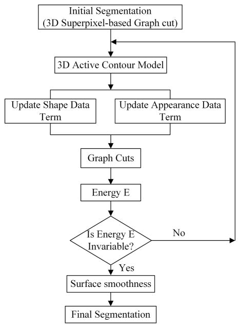
The proposed method consists of two parts that include graph cuts and active contour. Fig. 1 presents an overview of the proposed method.

Fig. 1.

The flowchart of the proposed segmentation method.

In this work, the superpixel is used as the basic processing unit for extracting the prostate surface. The pixels that have similar intensities and locations in the same slice are grouped together into a superpixel, which is used to compute robust local statistics. The usage of superpixel significantly reduces the computational and memory costs without sacrificing the accuracy due to the good adherence of superpixel to the boundary of the object.

The superpixels are connected to each other in the volume to form a 3D graph, which is a neighborhood system. A superpixel-based shape feature and superpixel-based gray feature are proposed to evaluate how likely a superpixel belongs to the prostate or background. Two superpixel-based smoothness terms are also proposed to construct the energy function. The initial segmentation is obtained by minimizing the energy function. However, the graph cuts usually miss the fine details or leak at the regions with weak edges. Therefore, a 3D active contour is introduced to solve this problem.

Although the classic active contour model has been used for medical image segmentation, it has a well-known problem of trapping at local minima when the initialization is not good enough, which limits its wide applications. In this work, the output of the graph cuts is used as an initialization of the active contour model in order to overcome this problem. The segmentation of the active contour method is then used to update the data terms of the graph cuts. Our hybrid method alleviates deficiencies of these two methods. These two parts are repeatedly performed until the energy of the graph cuts reaches the convergence. Finally, the output of the segmentation is post-processed to obtain smooth surface of the prostate.

B. Superpixel

Superpixel-based methods have many advantages for segmentation. First, a small number of superpixels reduce the computational cost and memory usage. Second, a superpixel with more pixels makes the superpixel-based feature more reliable and can minimize the risk of assigning wrong labels to the superpixels. Because of its improved performance over pixel-based methods, superpixel-based approaches [30]–[33] has been increasingly used in the field of computer vision. Superpixel segmentation provides an over-segmentation of an image by grouping pixels into homogeneous clusters based on intensity, texture, and other features. We choose super-pixel as the elementary processing unit of our segmentation method. For our prostate segmentation task, the generation of superpixel should meet two requirements. First, the generation of superpixel should be implemented efficiently. Second, the number and the size of superpixels should be in a reasonable range, which can be controlled by the user. From these points of view, the Simple Linear Iterative Clustering (SLIC) method [31] is adopted to segment each slice in order to obtain superpixels. The SLIC method has good performance and fast speed, as compared to other superpixel methods.

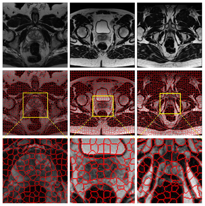
Fig. 2 shows the superpixel maps of three MR images, which are the slices at the mid-gland, base, and apex of the prostate. The figure demonstrates that the boundaries of superpixels correspond closely to the edges of the prostate. If our algorithm can pick up the right superpixels, the prostate boundary will be extracted properly.

Fig. 2.

Demonstration of the original MR images (top) and the corresponding superpixels (middle) for the slices at the mid-gland (left), base (middle), and apex (right) of the prostate. The region around the prostate is magnified to show the superpixels (bottom). Each MR image contains about 1,000 superpixels.

C. Graph Cuts

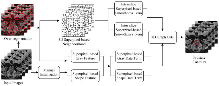
Fig. 4 shows the flowchart of the 3D superpixel-based graph cuts algorithm. First, the over-segmented superpixels are considered as the elementary processing units instead of pixels. The number of vertices and edges of the graph is significantly reduced compared to pixel-based graph cuts methods. Second, a 3D superpixel-based neighborhood system is built in the MR images. In this work, the Gaussian mixture model (GMM) [34] is used to build gray features for the data term. Due to the insufficient ability of handling images in which the background has similar intensity values to those of the prostate, a shape feature is also introduced for the data term in order to tackle this problem. Third, three key slices are selected and marked as an initialization to construct the shape feature for the data term. Fourth, two superpixel-based smoothness terms are proposed for the energy function, which are the inter-slice smoothness term and the intra-slice smoothness term. Finally, once the gray and shape features are obtained, an energy function is formulated, which can be optimized by graph cuts to obtain the prostate surface.

Fig. 4.

The framework of the 3D graph cuts algorithm.

Our energy function is formulated as follows:

$$E(l)=\sum _{s\in S}D(l_s)+\sum _{\{s_i,s_j\}\in N}V(l_{s_i},l_{s_j})$$ (1)

where N represents the 3D neighborhood system, S is a set of superpixels, {s_i, s_j} stands for two neighboring superpixels in the 3D neighborhood system. Data term D shows the likelihood of a superpixel assigned to the prostate or background. The smoothness term V measures the difference between two superpixels in the 3D neighborhood and encourages two similar neighboring superpixels to be assigned with the same label.

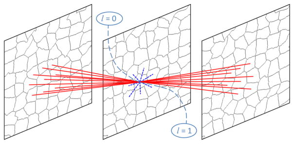
The 3D neighborhood system is constructed based on superpixels. Fig. 3 shows the 3D superpixel-based neighborhood system built on three successive slices.

Fig. 3.

The 3D superpixel-based neighborhood system in the 3D graph cuts algorithm. The red solid lines are inter-edges, while the blue dotted lines are intra-edges. The dash lines are terminal edges [24], l is the label of the superpixel. Label 1 corresponds to the prostate, while Label 0 represents the background.

The data term is constructed by combining gray and shape features in a weighted sum manner:

$$D(l_s)=(1-\alpha )D^{\mathit{gray}}(l_s)+\alpha D^{\mathit{shape}}(l_s)$$ (2)

where D^gray(l_s) and Dshape(l_s) are two unary-data penalty functions derived from gray and shape features. α controls the weight between the gray and shape features.

To model the gray data term of each superpixel s that belongs to either the prostate or background, a gray-level GMM is learned from the collected intensity values in the three key slices. A foreground prostate gray model p(G_s|l = 1) and a background gray model p(G_s|l = 0) are obtained based on the GMM, G_s represents the mean intensity of a superpixel. Once the p is obtained, the superpixel-based gray data term can be computed as follows:

$$D^{\mathit{gray}}(l_s=1)=-logp(G_s\mid l=1)$$ (3)

$$D^{\mathit{gray}}(l_s=0)=-logp(G_s\mid l=0)$$ (4)

With only the gray feature, it is difficult to obtain satisfactory segmentation of the prostate. Some background tissue with similar gray values can be labeled as the prostate. Therefore, a superpixel-based shape feature is introduced to resolve this problem.

To obtain the shape feature, a core shape is first introduced in our method. The basic idea is that the superpixels sit around or in the core shape have a high probability to be labelled as the prostate, and vice versa.

Three key slices are selected, which are at the base, apex and middle of the prostate. Four points are manually picked up for each of the three slices, as shown in Fig. 6. The core shapes of these three slices are obtained by fitting a Bezier curve based on the four points in each key slice (Blue points in Fig. 6).

Fig. 6.

On the left graph, the blue solid curves are prostate contours in the three key slices selected at the base, mid-gland and apex of the prostate. The blue dots are manually labelled markers. The red dotted lines are the true boundary of the prostate. The red dots on the red dotted lines are obtained using the interpolation of the corresponding blue dots in the 3D space. On the right graph, the red solid curve is the core shape, which is fitted based on the interpolated red dots.

To obtain the core shapes of the other slices, red dots of the other slices should be obtained first. The red dots are obtained based on linear interpolation of corresponding blue dots. Two ranges of linear interpolations are used to get the red dots. One is between the middle and apex key slices, the other is between the middle and base key slices. Once the red dots are obtained, the core shapes of these slices are generated by fitting a Bezier curve based on the interpolated red dots. All of these core shapes form a core shape surface, which will be used to generate the shape feature.

The prostate and background shape data terms are defined as follows.

$$D^{\mathit{shape}}(l_s=1)=-logp(S{H}_s\mid l=1)$$ (5)

$$D^{\mathit{shape}}(l_s=0)=-logp(S{H}_s\mid l=0)$$ (6)

where SH_s represents the mean value of the shape feature of a superpixel. Given SH_s of one superpixel s, the probability of labeling this superpixel s as the prostate is p(SH_s|l_s = 1), which is defined as:

$$p(S{H}_s\mid l_s=1)=1-p(S{H}_s\mid l_s=0)=\frac{1}{1+\mathit{exp}(-\gamma \ast (d-k_r))}$$ (7)

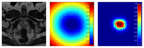
where d is the distance of a pixel to the core shape surface. The method of Felzenszwalb [35] is used to calculate d. k_r controls the fatness of the shape, while γ decides the gradient of d from the outside of the shape to the inside of the shape. Fig. 5 shows the superpixel-based shape data terms.

Fig. 5.

The superpixel-based shape data terms. Left: the original slice. Middle: the superpixel-based shape data term of the prostate. Right: the superpixel-based shape data term of the background. The penalties of the shape features will be used when the superpixels are assigned as the prostate or background. Blue color represents a low penalty, while red represents a high penalty.

The smoothness term is computed by combining two terms, which are the superpixel-based intra-slice smoothness term and the superpixel-based inter-slice smoothness term. The formulation of smoothness term is defined as follows.

$$V(l_{s_i},l_{s_j})=V^{\mathit{intra}}(l_{s_i},l_{s_j})+V^{\mathit{inter}}(l_{s_i},l_{s_j})$$ (8)

The intra-slice smoothness term V^intra(l_si, l_sj) evaluates the similarity of two neighboring superpixels connected by intra-edges in the 3D neighborhood system, which is defined as:

$$V^{\mathit{intra}}(l_{s_i},l_{s_j})=(1-\delta (l_{s_i},l_{s_j}))e^{-\beta {\Vert G_i-G_j\Vert }^2}$$ (9)

δ is the Kronecker delta function that encourages penalty to be considered only for edges across the segmentation boundary. δ(l_sj ≠ l_si) = 0, if two labels are different. G_i represents the gray expectations of all pixels in a superpixel i. ||·|| is the L₂ norm, β is a constant parameter that weights the gray gradient, and is set as β = (2 <||G_i−G_j||²>)⁻¹, where < · > denotes expectation over all pairs of neighboring superpixels in the 3D MR images.

The inter-slice smoothness term V^inter(l_si, l_sj) evaluates the difference of two neighboring superpixels connected by inter-edges in the 3D neighborhood system, which is defined as:

$$V^{\mathit{inter}}(l_{s_i},l_{s_j})=(1-\delta (l_{s_i},l_{s_j}))\frac{A(s_i\cap s_j)}{A(s_i\cup s_j)}$$ (10)

where A(s_i ∩ s_j) stands for the area of intersection of two superpixels connected by inter-edge, and A(s_i ∪ s_j) represents the area of union. This term encourages the superpixels in different slices with similar shapes and locations to be assigned as the same labels.

Once data and smoothness terms are obtained, the prostate will be segmented by finding a 3D graph cut that minimizes the energy function. However, following this efficient way does not mean that the segmentations are perfect. This is because the graph cuts may make segmentation leaks at weak edges. To overcome these shortcomings of graph cuts, an active contour model is introduced in the proposed method.

D. Active Contour Model

Chan and Vese [20] proposed an algorithm called active contours without edges, which has been studies mainly in the context of 2D images. In this work, we present a 3D Chan-Vese active contour model to extract the prostate surface.

The model will find a surface that divides an MR image volume into two regions, which are the prostate and the background. The 3D active contour not only makes segmentation more smoothness, but also alleviates the deficiency of inaccurate boundaries obtained from graph cuts, especially, when the initial superpixels fail to accurately find the boundary of the prostate.

It can be difficult to segment the boundary of the prostate at the base and apex regions. Therefore, a user intervention may be helpful to determine the true boundary of the prostate at those two regions. The input points of the user on the apex and base slices are useful for accurate segmentation of the prostate. In the 3D ACM, the surface at the apex and base are constrained in an area surrounding the points of the user interventions. Therefore, for the apex and base slices, we only focus on the detection of the prostate boundary in a local region around the core shapes that are interpolated from the initialization points labeled by the user.

E. Hybrid Approach of Graph Cuts and Active Contour Model

In our work, the initial 3D segmentation is generated by applying the 3D superpixel-based graph cuts algorithm. The user picks up three key slices and marks key points for each of the three slices. A core shape surface is obtained based on these marked key points. The gray data term and shape data term are built based on these three selected key slices and the core shape surface. The smoothness terms are built based on 3D superpixel-based neighborhood system. Once data and smoothness terms are obtained, the superpixel-based energy function can be minimized by graph cuts to extract the prostate surface C₀, which is used as the initial segmentation for the active contour model.

Since the initial prostate surface C₀ is obtained by graph cuts, it sometimes misses the fine details and leaks at the regions with weak boundaries, which could be critical for MR prostate images. Therefore, the 3D active contour model is introduced to solve this problem. The output of the graph cuts C₀ is used as the input of the 3D active contour model. C₀ is close to the true surface of the prostate, so the output prostate surface C_ac of the 3D active contour model will not be far from the ground truth.

As C₀ is obtained only based on the three key slices, it is not good enough to extract the prostate surface. Therefore, the surface C_ac is used to update the gray and shape data terms of the graph cuts algorithm. The 3D graph cuts and 3D active contour are iteratively performed until the surface solution has converged or the maximum number of the iterations has been reached.

F. Evaluation Metrics

Our segmentation method was evaluated using four quantitative metrics, which are Dice similarity coefficient (DSC), relative volume difference (RVD), Hausdorff distance (HD), and average surface distance (ASD) [4], [36]. The RVD is used to evaluate whether the algorithm tends to over-segment or under-segment the prostate. RVD is negative, if the algorithm over-segments the prostate and vice versa. To compare our method with the methods proposed by Qiu [4], [9], the mean absolute distance (MAD) is also used.

III. Experimental Results

A. Data

In this work, 43 prostate volumes of T2-weighted MR images from Emory University Hospital were used in the experiments. All subjects were scanned at 1.5 T and 3.0 T with three Siemens Magnetom systems, which are Aera, Trio Tim, and Avanto. No endorectal coil was used for our data acquisition. The repetition time (TR) varies from 1000 ms to 7500 ms, while echo time (TE) varies from 91 ms to 120 ms. The original slice spacing varies from 1 mm to 6 mm. This data set allows us to test the robustness of the algorithm. To better visualize and analyze the data, an isotropic volume is obtained for each MR data using windowed sinc interpolation. The voxel size is typically 0.625 mm³, 0.875 mm³, or 1 mm³. The size of the transverse images varies from 320×320 to 256×256. Each slice was manually segmented by two experienced radiologists for assessing the inter-observer and intra-observer variability. To avoid the situation that the radiologist remembers previous manual segmentation, any two manual segmentations were performed at least one week apart. Majority voting is adopted to fuse the labels from different ground truths, which were manually segmented by the two radiologists. The segmentation result from our algorithm is compared with the six ground truths from the two radiologists. The mean DSC varies from 88.33% to 90.84%, while the mean ASD varies from 1.68 mm to 1.86 mm. The DSC is used to evaluate the inter- and intra-observer variability. For the intra-observer variability, the DSC of each two ground truths varies from 87.38% to 93.16%. For the inter-observer variability, the DSC between two radiologists is 90.52%.

We also validated our algorithm on a publicly available data set called the PROMISE12 Challenge [37], which contains 30 prostate T2 MR images. The ground truths of these 30 images are not available. The user must submit their segmentation results to the PROMISE12 website in order to obtain the quantitative evaluation results and ranking. This data set was obtained from multi-center and multi-vendor studies, which have different acquisition protocols (i.e., different slice thickness, with/without endorectal coil).

B. Implementation Details

The main algorithm was implemented in MATLAB codes and the graph cut was implemented in C++ codes. The algorithm runs on a Windows 7 desktop with an Intel Xeon E5-2687W CPU (3.4GHz) and 128 GB memory. Our code is not optimized and does not use multi-thread, GPU acceleration or parallel programming.

C. Qualitative Results

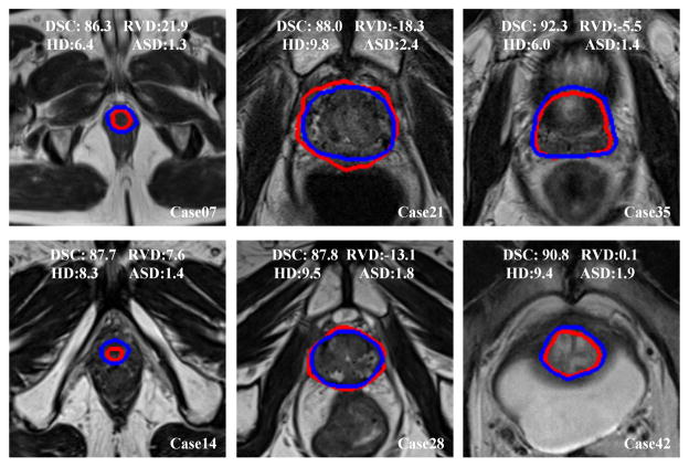
The qualitative results from six prostate volumes are shown in Fig. 7. Blue curves are the manually segmented ground truth by the radiologist, while the red curves are the segmentation of the proposed method.

Fig. 7.

Qualitative evaluation of the prostate segmentation on six MR volumes. We choose the volumes every seventh case. The blue curves are the manually labeled ground truth, while the red curves are the segmentations of the proposed method for the apex (left), mid-gland (middle), and base (right) of the prostate. The values of DSC(%), RVD(%), HD(mm), and ASD(mm) of each case are overlaid on the images.

Fig. 8 shows the 3D overlay visualization of the manual segmentation and our segmentation of the prostate volume, indicating that the segmentation obtained by the proposed well overlaps with the ground truth.

Fig. 8.

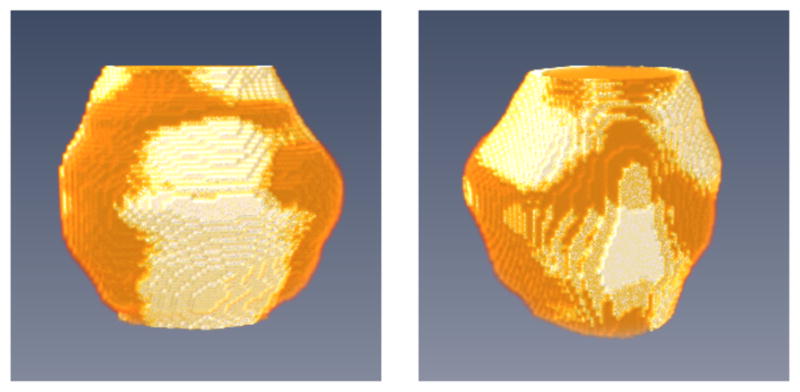
3D visualization of the segmented prostate (white regions) compared to the manual ground truth (gold regions) in two different views.

D. Quantitative Results on Our Data Set

Table I shows the quantitative evaluation results from 43 MR image volumes. For this experiment, each prostate volume was divided into three sub-regions, i.e., the base, apex, and middle regions, which contain 30%, 30%, and 40% slices, respectively. The values of four metrics of each sub-region are also posted in the table. Our approach yielded a DSC of 89.3±1.9%, while the minimal DSC is 86.0% and the maximum DSC is 92.3%. The DSC indicates that our method segments all the 43 prostates with a relatively high accuracy and low standard deviation. The average surface distance is 1.7±0.4 mm, indicating that the proposed method can segment the prostate gland with a relatively low error. For the 43 volumes, the HD, which measures the maximum distance between two surfaces, is 8.7±2.7 mm. The average RVD of our method is 0.7%, which shows that the result obtained by the proposed method has a good balance between over-segmentation and under-segmentation. The low standard deviation of the computed four metrics shows the robustness and repeatability of the proposed algorithm. The quantitative evaluation agrees with the conclusions from the visual observation of the experimental results.

TABLE I.

Quantitative results of the segmentation. The table shows the results of the whole gland and the three sub-regions, which are the base, apex, and mid-gland regions. DSC: Dice similarity coefficient (%), RVD: relative volume difference (%), HD: Hausdorff distance (mm), and ASD: average surface distance (mm)

Vol#	Whole gland				Apex				Mid-gland				Base
	DSC	RVD	HD	ASD	DSC	RVD	HD	ASD	DSC	RVD	HD	ASD	DSC	RVD	HD	ASD
1	91.0	−4.0	6.8	1.4	90.4	−0.3	6.0	1.2	92.7	−9.3	5.4	1.3	88.3	3.7	6.8	1.7
2	90.1	−7.2	6.1	1.4	86.7	19.7	5.0	1.5	93.7	−8.7	6.1	1.1	85.1	−21.1	5.2	1.8
3	86.6	11.7	10.3	1.8	91.4	−3.7	4.5	1.0	91.3	1.8	7.1	1.4	76.0	42.6	10.3	3.0
4	91.3	−2.4	7.3	1.3	89.9	8.8	4.9	1.3	94.6	0.9	5.0	1.1	84.3	−18.0	9.9	1.9
5	88.0	7.5	9.8	1.7	89.9	−1.7	7.1	1.2	92.1	−2.7	8.1	1.4	78.6	40.8	9.8	2.9
6	87.5	6.0	7.0	1.6	82.9	11.9	6.6	1.8	91.0	0.1	6.7	1.4	85.0	12.1	7.0	1.7
7	86.3	21.9	6.4	1.3	83.0	28.3	4.4	1.3	92.4	5.7	3.0	0.9	80.1	44.1	6.4	1.9
8	89.1	−4.4	6.7	1.5	85.9	−16.5	4.9	1.5	90.9	−12.0	6.7	1.5	88.3	15.8	5.0	1.6
9	91.8	1.9	13.0	1.8	89.3	1.4	9.2	1.6	92.4	4.8	13.0	2.0	92.2	−3.1	8.2	1.6
10	89.3	3.3	7.6	1.5	80.1	25.2	8.6	2.0	92.1	2.5	8.3	1.4	90.2	−7.2	6.0	1.4
11	89.2	0.6	7.0	1.4	87.9	5.9	4.4	1.3	92.9	−6.9	6.6	1.1	84.0	10.1	7.3	1.9
12	88.5	7.9	13.1	2.1	90.2	−10.7	5.8	1.5	93.0	−1.7	8.4	1.4	79.9	45.7	15.3	3.6
13	88.1	9.6	5.0	1.2	82.9	3.5	5.0	1.5	91.1	3.9	3.6	1.0	87.9	20.5	4.5	1.3
14	87.7	7.6	8.3	1.4	79.0	12.0	5.4	1.9	91.8	−5.8	5.0	1.1	87.8	21.4	8.3	1.6
15	86.3	−7.0	12.2	2.3	82.8	−24.8	8.1	2.4	88.7	−17.2	9.4	2.1	85.1	20.4	12.2	2.7
16	89.2	−3.2	10.0	2.2	87.5	24.5	7.3	2.2	93.0	−2.8	10.6	1.8	82.3	−25.0	10.0	3.2
17	89.8	3.9	6.4	1.4	88.2	23.4	6.0	1.5	91.7	0.8	6.8	1.4	86.3	−7.7	6.8	1.7
18	91.2	−6.2	9.4	1.8	88.8	−7.6	9.4	1.9	93.3	−4.4	8.5	1.6	89.0	−8.8	7.5	2.1
19	91.3	1.4	7.1	1.1	83.8	1.2	7.1	1.6	95.3	0.9	4.0	0.8	89.3	2.8	5.2	1.1
20	91.4	−2.2	6.3	1.2	88.4	17.6	5.0	1.1	93.3	−4.4	5.0	1.0	89.9	−6.0	6.3	1.4
21	88.0	−18.3	9.8	2.4	85.6	−21.9	6.8	2.0	87.9	−21.1	9.8	2.8	89.2	−13.4	8.1	2.4
22	91.8	1.6	11.9	2.1	87.1	24.7	8.8	2.7	93.3	−2.1	11.9	2.1	92.4	−6.3	8.9	1.9
23	90.1	−1.3	9.6	2.1	87.0	−7.3	9.4	2.3	93.0	0.4	8.1	1.8	87.3	0.4	10.0	2.5
24	89.8	−9.5	7.7	1.6	89.3	−11.3	5.4	1.3	91.3	−8.7	7.7	1.6	86.9	−9.5	7.0	1.8
25	87.8	9.0	9.9	1.7	83.9	11.1	6.7	2.1	91.2	4.7	8.6	1.6	82.2	21.3	14.1	1.8
26	91.4	0.7	15.0	1.8	90.8	−6.0	6.1	1.8	93.0	4.3	15.0	1.8	87.2	0.8	9.2	1.9
27	90.0	−0.3	7.5	1.3	88.1	−11.6	5.4	1.4	93.5	−5.6	4.5	1.1	85.0	20.3	7.5	1.7
28	87.8	−13.1	9.5	1.8	80.7	−28.6	7.0	2.1	94.0	−8.3	5.5	1.2	81.5	−10.5	9.5	2.6
29	89.7	−8.9	12.7	2.2	91.8	−4.7	5.7	1.5	92.5	−10.3	14.2	1.8	82.2	−9.8	11.8	3.6
30	90.3	4.6	15.0	3.0	85.4	2.5	13.7	3.6	94.8	0.9	12.1	2.0	84.7	15.8	15.3	4.1
31	86.6	14.4	13.1	2.2	90.0	8.3	5.1	1.6	91.3	1.9	8.5	1.7	71.7	61.6	15.8	4.1
32	90.6	2.2	6.0	1.3	86.7	−6.8	5.5	1.3	92.3	−1.0	5.4	1.3	90.2	11.5	6.0	1.5
33	91.7	1.3	10.5	1.9	87.2	7.9	9.9	2.5	93.5	−0.8	10.5	1.7	92.5	−0.9	5.9	1.6
34	89.5	14.2	5.1	1.4	86.5	26.7	5.0	1.4	92.4	1.6	4.7	1.1	88.0	22.5	5.1	1.7
35	92.3	−5.5	6.0	1.4	90.3	−4.1	6.7	1.5	93.0	−9.3	6.1	1.4	92.7	−1.9	5.9	1.5
36	92.2	−2.4	8.5	2.0	90.1	−4.3	8.0	2.1	92.8	−6.5	10.0	2.1	93.0	5.5	6.0	1.9
37	91.9	−3.1	8.6	1.6	88.7	−4.4	8.6	1.9	94.7	−0.9	7.6	1.3	89.3	−6.2	8.5	1.9
38	86.0	0.4	5.7	1.4	81.9	24.9	5.0	1.5	90.2	−7.7	7.0	1.2	83.6	−3.6	5.7	1.6
39	87.0	−1.7	7.7	2.0	87.4	−8.6	7.1	1.8	88.9	−15.0	7.7	1.9	84.3	26.6	8.1	2.4
40	87.3	−10.7	6.2	1.4	88.8	−0.7	4.1	1.2	87.9	−17.1	6.6	1.5	83.8	−7.0	7.1	1.6
41	87.1	−6.9	6.6	1.6	87.4	11.0	5.8	1.4	88.4	−9.9	7.7	1.7	83.9	−16.4	6.2	1.6
42	90.8	0.1	9.4	1.9	90.4	19.2	8.6	2.0	92.7	−1.2	12.2	1.8	87.1	−15.8	10.3	2.3
43	87.4	17.9	7.3	1.7	83.8	37.5	7.7	2.1	90.4	12.1	7.0	1.5	84.5	9.5	6.4	1.8
Avg.	89.3	0.7	8.7	1.7	86.9	4.0	6.7	1.7	92.1	−3.6	7.8	1.5	85.9	6.5	8.3	2.1
Std.	1.9	8.2	2.7	0.4	3.2	15.5	1.9	0.5	1.8	6.9	2.8	0.4	4.5	19.9	2.9	0.7

E. Quantitative Results on PROMISE12 Data Set

Our proposed method was ranked at the second place in the PROMISE12 Challenge¹. Compared to the method at the first place, our method has much smaller standard deviation and is actually the smallest among all methods, indicating the robustness of our method.

The proposed approach yielded a DSC of 87.03±3.21%, an average boundary distance of 2.14±0.35 mm, a 95% HD of 5.04±1.03 mm, and a volume difference of 4.28±9.27%, for the whole prostate gland. The DSCs of 83.52±6.32% and 81.53±6.89% were found at the base and apex regions, respectively.

F. Comparison with Other Methods

Eleven state-of-the-art prostate segmentation methods [3], [4], [8]–[10], [13]–[16], [18], [38] were chosen as the benchmark to evaluate our method. The comparisons of these 11 methods with our method are provided in Table II. DSC and MAD are chosen as metrics to evaluate the performance of these methods. The results of these five methods [3], [4], [10], [16], [38] were from Qiu’s paper [4]. It should be noted that since all of the results evaluated on different data sets, a direct comparison is difficult. The results were reported as mean ± standard deviation. The hyphen means that the corresponding measures are not reported in the respective papers.

TABLE II.

Comparison with 11 other prostate MR segmentation methods

Paper	Year	DSC(%)	MAD(mm)	Time(s)	Type
Klein [10]	2008	85.0–88.0	-	900	automatic
Gao [38]	2010	84.0±3.0	-	-	automatic
Martin [16]	2010	84	2.4	240	automatic
Langerak [13]	2010	87	-	480	automatic
Toth [3]	2012	88.0±5.0	1.5±0.8	150	automatic
Liao [8]	2013	86.7±2.2	-	-	automatic
Xie [14]	2014	86	-	-	automatic
Guo [18]	2014	89.1±3.6	-	60–120	automatic
Qiu [9]	2014	(89.2–89.3)±(3.2–3.3)	(3.2–3.3)±(0.8–1.0)	50	semi-automatic
Qiu [4]	2014	88.5±3.5	1.8±0.8	5	semi-automatic
Korsager [15]	2015	88	-	-	semi-automatic
Ours	2015	89.3±1.9	1.6±0.3	35	semi-automatic

Our method achieved a mean DSC of 89.3±1.9%, which is the highest DSC with the lowest standard deviation. Toth’s method has a little higher MAD than ours. But our method has the lowest standard deviation of the MAD. With a GPU optimization, Qiu’s method [4] has a higher efficiency of within 5 seconds compared to 35 seconds of our method that does not use GPU acceleration.

Among these methods, two methods [4], [9] have the top performance, and also posted their quantitative results on the three sub-regions in their papers. Therefore, we chose these two methods for the further comparison.

For the first method [4], Table III shows the comparison results in term of DSC on the three sub-regions. Qiu’s method yields a higher DSC than ours at the middle regions. But our method has a higher DSC than Qiu’s method for the base and apex regions as well as the whole prostate. Moreover, our method has a lower standard deviation for the whole prostate, middle, and apex regions, which yields a consistent DSC. The testing for statistical significance was performed at the whole prostate and the three sub-regions between the two methods in terms of DSC, HD, and MAD. The Bonferroni correction is used to counteract the problem of multiple comparisons. The analysis shows that there is a statistically significant difference at the apex region in terms of DSC and HD, and at the middle region in terms of HD and MAD.

TABLE III.

Evaluation of the three sub-regions: base, apex, and mid-gland of the prostate. The DSCs with standard deviation of Qius method are used for the comparison

	Total	Base	Mid	Apex	#Volume
Qiu [4]	88.5±3.5	83.7±4.2	92.6±2.8	84.0±4.0	30
Ours	89.3±1.9	85.9±4.5	92.1±1.8	86.9±3.2	43

For the second method [9], the testing for statistical significance was also performed on the whole prostate and three sub-regions in terms of DSC, HD, and MAD. The analysis shows that there is no statistically significant difference on all of DSCs. However, there is a statistically significant difference in terms of HD and MAD on the whole prostate and three subregions, except at the base region in terms of HD.

G. Parameter Sensitivity

In our experiments, the parameters were set empirically at first. Then we optimized one parameter at a time while other parameters were fixed. The DSC was used to evaluate the performance of the segmentation for the choice of the parameters. Once the parameters are determined, they were fixed in all of the experiments.

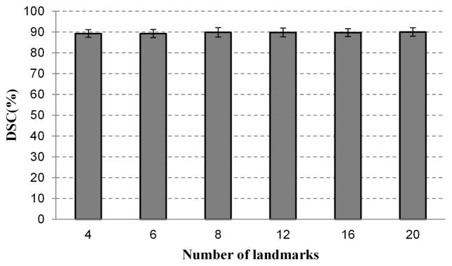
To evaluate the influence of the number of the points on one key slice, the DSC was obtained from the segmentation experiments with different parameter settings for all the 43 volumes data, as shown in Fig. 9. The DSC varies only in a small range, indicating that the proposed segmentation is robust and insensitive to the number of markers.

Fig. 9.

The effect of the number of the points on the segmentation performance. When the number of the points varies from 4 to 20, the DSC has very small changes. The proposed method is insensitive to the number of mark points picked by the user.

Extensive segmentation experiments were performed to assess whether our algorithm is sensitive to the selection of the apex, base, and middle slices. In our method, the user selects three key slices. To evaluate the effect of the selection of the middle slice, four slices around the middle slice M(i) are selected as the current middle slice to run the algorithm individually. These four slices are M(i − 2), M(i − 1), M(i + 1), and M(i + 2). Fig. 10(a) shows the evaluation result of the selection of the middle slice. Besides the evaluation of middle slice, the selections of the apex slice and base slice are also evaluated, which are shown in Figs. 10(b) and 10(c). The result shows that the proposed method is not sensitive to the selections of the apex, based, and middle slices.

Fig. 10.

The effect of selecting three key slices on the segmentation performance. Five successive slices around each key slice are chosen to be the key slices individually. The mean DSC and standard deviation are from the 43 MR volumes.

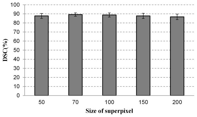
Superpixels with a smaller size are more homogeneous but increase the computational cost. Larger superpixels reduce the computational cost more than smaller superpixels, but it may straddle the boundary between two objects. To test the effect of superpixel size on segmentation performance, our method is tested on pre-segmented superpixels with different sizes. The parameter of the SLIC is tuned to obtain several sizes varying from 50 to 200 pixels. Fig. 11 shows the dependency of segmentation performance on the superpixel size. Forty three volumes are used in this experiment, while five superpixel sizes are used for each MR volume. The proposed method provides similar DSC ratios when the size is in the range from 50 to 100. In the all of our experiments, 70 is selected as the superpixel size for all the experiments, which gives a good compromise between the efficiency and performance. When the size increases to 150 or 200, the DSC ratios decrease slightly, as shown in Fig. 11.

Fig. 11.

The effect of superpixel size on the segmentation performance. Five sizes of superpixel are chosen to test the ability of the segmentation method, which are 50, 70, 100, 150 and 200 pixels.

Experiments were carried out to compare the performance of the 3D graph cuts algorithm, 3D active contour model, and the proposed hybrid method. For the 3D superpixel-based graph cuts algorithm, the gray and shape data terms are built based on the three key slices. There is no iteration for minimizing the energy function, which means the graph cuts is only performed once. For the 3D active contour model, the core shapes are used as the initialization input.

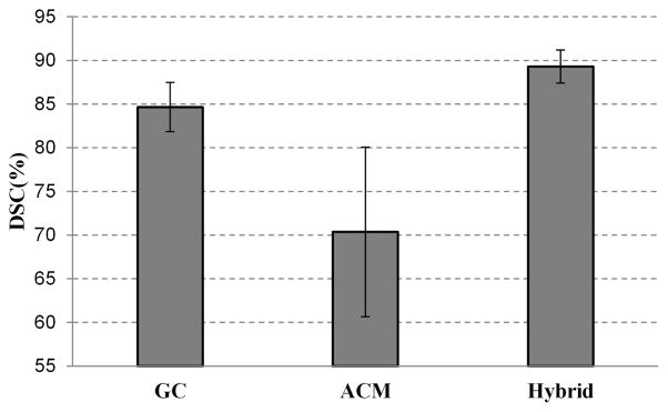
Fig. 12 shows the average DSC of the three methods for 43 MRI volumes. The DSC of the 3D ACM is 70.4%, which is not ideal. This is because the initialization is not good for 3D ACM. For the 3D graph cuts algorithm, the DSC is better than that of ACM, which is 84.6%. With the combination of graph cuts and active contour model, the quality of the segmentation is improved, which is increased to 89.3%. This figure also shows that the output segmentation of the graph cuts is competent to be a good initialization for the active contour model.

Fig. 12.

Comparison of three segmentation methods: graph cuts only, active contour model only, and the hybrid approach of the two methods.

IV. Conclusion

A. Conclusion

A hybrid 3D method that combines a 3D graph cuts and a 3D active contour model in a loop manner is proposed to segment prostate MR images. By utilizing a surface style instead of the curve-by-curve style, the proposed segmentation method is able to utilize the full 3D special information to extract the surface of the prostate. We have also approached the problem of prostate segmentation from a novel point of view by using superpixel instead of pixel. Our method profits from superpixel at two aspects: 1) it makes the shape and gray features robust, which reduces the risk of labeling the superpixels with wrong labels. Many new features can be developed based on the superpixels, which is one of our future works. 2) The proposed method reduces the computational and memory costs, which makes the 3D volume segmentation is tractable. We believe that the superpixel-based method can be applied for medical images of most body regions and other different image modalities. The experimental results show that the proposed method outperforms the state-of-the-art methods in terms of accuracy and robustness.

B. Limitation

The proposed method is based on an initial over-segmentation called superpixel. Therefore, if the initial over-segmentation does not provide a good adherence to the prostate boundary, the proposed method may have a decreased performance. Fortunately, other works [31], [39] have been developed or are under development to improve the accuracy of how to generate superpixels, which will also improve the performance of our segmentation algorithm.

In addition, this work is a semi-automatic method, which requires the user interventions for initialization. It is important to develop a fully automatic segmentation method, which can be implemented by obtaining the initialization in an automatic manner. Atlas-based methods and machine learning methods are potential solutions for automatically obtaining the approximate location of the prostate. Our future work will focus on developing robust, accurate, fully automatic methods.

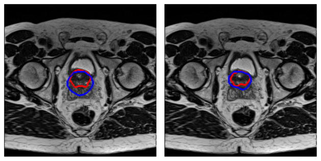
The method may need to improve the performance for image volumes that contain sudden changes between adjacent slices of the prostate, for example, when two successive slices have very different shapes and sizes of the prostate. This is not caused by initial superpixel segmentation but by the initial core shape of the initialization. The core shape is obtained by interpolation, which assumes that two adjacent slices have a similar shape and size for the prostate. As shown in Fig. 13, if there is a sudden change in the shape and the size of the prostate at the bladder neck (blue contours), the sudden variation may lead to segmentation errors at that region. This problem can be solved by adding more landmarks on the slices that have sudden changes of the prostate.

Fig. 13.

Prostate segmentation of two adjacent slices at the bladder neck (Blue: the ground truth from manual segmentation. Red: the segmentation by the algorithm).

C. Discussion

In the experiment as shown in Fig. 9, we have evaluated the effect of the user initialization. The proposed method with more mark points performs slightly better than that of few mark points. Nonetheless, it still extracts the good enough surface of the prostate with even only four mark points on the key slice. In general, the proposed algorithm could reliably extract the prostate surfaces from MR volumes if the mark points cover the key feature location of the prostate.

The proposed segmentation method is implemented without optimization. To make it more practical in the clinical application, the multithread implementation of the method is one solution. Liu et al. [40] have proposed a novel adaptive bottom-up approach to parallelize the graph cuts algorithm. We will investigate the parallelization of our proposed method in the future. In addition, 3D superpixel based method has lower computational complexity for segmenting prostate, which is also our future work. We believe that our semi-automatic segmentation method can have many applications in prostate imaging.

References

- 1.Qiu W, Yuan J, Ukwatta E, Sun Y, Rajchl M, Fenster A. Fast globally optimal segmentation of 3d prostate mri with axial symmetry prior. Medical image computing and computer-assisted intervention: MICCAI. 2013;16(Pt 2):198–205. doi: 10.1007/978-3-642-40763-5_25. [DOI] [PubMed] [Google Scholar]
- 2.Litjens G, Debats O, van de Ven W, Karssemeijer N, Huisman H. Medical Image Computing and Computer-Assisted Intervention–MICCAI 2012. Springer; 2012. A pattern recognition approach to zonal segmentation of the prostate on mri; pp. 413–420. [DOI] [PubMed] [Google Scholar]
- 3.Toth R, Madabhushi A. Multifeature landmark-free active appearance models: Application to prostate mri segmentation. Medical Imaging, IEEE Transactions on. 2012;31(8):1638–1650. doi: 10.1109/TMI.2012.2201498. [DOI] [PubMed] [Google Scholar]
- 4.Qiu W, Yuan J, Ukwatta E, Sun Y, Rajchl M, Fenster A. Prostate segmentation: An efficient convex optimization approach with axial symmetry using 3-d trus and mr images. IEEE transactions on medical imaging. 2014;33(4):947–960. doi: 10.1109/TMI.2014.2300694. [DOI] [PubMed] [Google Scholar]
- 5.Khalvati F, Salmanpour A, Rahnamayan S, Rodrigues G, Tizhoosh H. Inter-slice bidirectional registration-based segmentation of the prostate gland in mr and ct image sequences. Medical physics. 2013;40(12):123503. doi: 10.1118/1.4829511. [DOI] [PubMed] [Google Scholar]
- 6.Fei B, Yang X, Nye JA, Aarsvold JN, Raghunath N, Cervo M, Stark R, Meltzer CC, Votaw JR. Mr/pet quantification tools: Registration, segmentation, classification, and mr-based attenuation correction. Medical physics. 2012;39(10):6443–6454. doi: 10.1118/1.4754796. [DOI] [PMC free article] [PubMed] [Google Scholar]
- 7.Makni N, Iancu A, Colot O, Puech P, Mordon S, Betrouni N. Zonal segmentation of prostate using multispectral magnetic resonance images. Medical physics. 2011;38(11):6093–6105. doi: 10.1118/1.3651610. [DOI] [PubMed] [Google Scholar]
- 8.Liao S, Gao Y, Oto A, Shen D. Medical Image Computing and Computer-Assisted Intervention–MICCAI 2013. Springer; 2013. Representation learning: a unified deep learning framework for automatic prostate mr segmentation; pp. 254–261. [DOI] [PMC free article] [PubMed] [Google Scholar]
- 9.Qiu W, Yuan J, Ukwatta E, Sun Y, Rajchl M, Fenster A. Dual optimization based prostate zonal segmentation in 3d mr images. Medical image analysis. 2014;18(4):660–673. doi: 10.1016/j.media.2014.02.009. [DOI] [PubMed] [Google Scholar]
- 10.Klein S, van der Heide UA, Lips IM, van Vulpen M, Staring M, Pluim JP. Automatic segmentation of the prostate in 3d mr images by atlas matching using localized mutual information. Medical physics. 2008;35(4):1407–1417. doi: 10.1118/1.2842076. [DOI] [PubMed] [Google Scholar]
- 11.Chandra SS, Dowling JA, Shen KK, Raniga P, Pluim JP, Greer PB, Salvado O, Fripp J. Patient specific prostate segmentation in 3-d magnetic resonance images. Medical Imaging, IEEE Transactions on. 2012;31(10):1955–1964. doi: 10.1109/TMI.2012.2211377. [DOI] [PubMed] [Google Scholar]
- 12.Warfield SK, Zou KH, Wells WM. Simultaneous truth and performance level estimation (staple): an algorithm for the validation of image segmentation. Medical Imaging, IEEE Transactions on. 2004;23(7):903–921. doi: 10.1109/TMI.2004.828354. [DOI] [PMC free article] [PubMed] [Google Scholar]
- 13.Langerak TR, Van Der Heide U, Kotte AN, Viergever M, Van Vulpen M, Pluim JP, et al. Label fusion in atlas-based segmentation using a selective and iterative method for performance level estimation (simple) Medical Imaging, IEEE Transactions on. 2010;29(12):2000–2008. doi: 10.1109/TMI.2010.2057442. [DOI] [PubMed] [Google Scholar]
- 14.Xie Q, Ruan D. Low-complexity atlas-based prostate segmentation by combining global, regional, and local metrics. Medical physics. 2014;41(4):041909. doi: 10.1118/1.4867855. [DOI] [PubMed] [Google Scholar]
- 15.Korsager AS, Fortunati V, van der Lijn F, Carl J, Niessen W, Østergaard LR, van Walsum T. The use of atlas registration and graph cuts for prostate segmentation in magnetic resonance images. Medical physics. 2015;42(4):1614–1624. doi: 10.1118/1.4914379. [DOI] [PubMed] [Google Scholar]
- 16.Martin S, Troccaz J, Daanen V. Automated segmentation of the prostate in 3d mr images using a probabilistic atlas and a spatially constrained deformable model. Medical physics. 2010;37(4):1579–1590. doi: 10.1118/1.3315367. [DOI] [PubMed] [Google Scholar]
- 17.Toth R, Tiwari P, Rosen M, Reed G, Kurhanewicz J, Kalyanpur A, Pungavkar S, Madabhushi A. A magnetic resonance spectroscopy driven initialization scheme for active shape model based prostate segmentation. Medical Image Analysis. 2011;15(2):214–225. doi: 10.1016/j.media.2010.09.002. [DOI] [PMC free article] [PubMed] [Google Scholar]
- 18.Guo Y, Gao Y, Shao Y, Price T, Oto A, Shen D. Deformable segmentation of 3d mr prostate images via distributed discriminative dictionary and ensemble learning. Medical physics. 2014;41(7):072303. doi: 10.1118/1.4884224. [DOI] [PMC free article] [PubMed] [Google Scholar]
- 19.Kass M, Witkin A, Terzopoulos D. Snakes: Active contour models. International journal of computer vision. 1988;1(4):321–331. [Google Scholar]
- 20.Chan TF, Vese LA. Active contours without edges. Image processing, IEEE transactions on. 2001;10(2):266–277. doi: 10.1109/83.902291. [DOI] [PubMed] [Google Scholar]
- 21.Tsai A, Yezzi A, Jr, Wells W, Tempany C, Tucker D, Fan A, Grimson WE, Willsky A. A shape-based approach to the segmentation of medical imagery using level sets. Medical Imaging, IEEE Transactions on. 2003;22(2):137–154. doi: 10.1109/TMI.2002.808355. [DOI] [PubMed] [Google Scholar]
- 22.Qiu W, Yuan J, Ukwatta E, Tessier D, Fenster A. Three-dimensional prostate segmentation using level set with shape constraint based on rotational slices for 3d end-firing trus guided biopsy. Medical physics. 2013;40(7):072903. doi: 10.1118/1.4810968. [DOI] [PubMed] [Google Scholar]
- 23.Boykov Y, Veksler O, Zabih R. Fast approximate energy minimization via graph cuts. Pattern Analysis and Machine Intelligence, IEEE Transactions on. 2001;23(11):1222–1239. [Google Scholar]
- 24.Boykov YY, Jolly M-P. Interactive graph cuts for optimal boundary & region segmentation of objects in nd images. Computer Vision, 2001. ICCV 2001. Proceedings. Eighth IEEE International Conference on; IEEE; 2001. pp. 105–112. [Google Scholar]
- 25.Egger J. Pcg-cut: graph driven segmentation of the prostate central gland. PloS one. 2013;8(10):e76645. doi: 10.1371/journal.pone.0076645. [DOI] [PMC free article] [PubMed] [Google Scholar]
- 26.Mahapatra D, Buhmann JM. Prostate mri segmentation using learned semantic knowledge and graph cuts. Biomedical Engineering, IEEE Transactions on. 2014;61(3):756–764. doi: 10.1109/TBME.2013.2289306. [DOI] [PubMed] [Google Scholar]
- 27.Xu N, Ahuja N, Bansal R. Object segmentation using graph cuts based active contours. Computer Vision and Image Understanding. 2007;107(3):210–224. [Google Scholar]
- 28.Huang R, Pavlovic V, Metaxas DN. A graphical model framework for coupling mrfs and deformable models. Computer Vision and Pattern Recognition, 2004. Proceedings of the 2004 IEEE Computer Society Conference on; IEEE; 2004. pp. 739–746. [Google Scholar]
- 29.Uzunbaş MG, Chen C, Zhang S, Pohl KM, Li K, Metaxas D. Collaborative multi organ segmentation by integrating deformable and graphical models. Medical image computing and computer-assisted intervention: MICCAI. International Conference on Medical Image Computing and Computer-Assisted Intervention. 2013;16(Pt 2):157–164. doi: 10.1007/978-3-642-40763-5_20. [DOI] [PMC free article] [PubMed] [Google Scholar]
- 30.Felzenszwalb PF, Huttenlocher DP. Efficient graph-based image segmentation. International Journal of Computer Vision. 2004;59(2):167–181. [Google Scholar]
- 31.Achanta R, Shaji A, Smith K, Lucchi A, Fua P, Susstrunk S. Slic superpixels compared to state-of-the-art superpixel methods. Pattern Analysis and Machine Intelligence, IEEE Transactions on. 2012;34(11):2274–2282. doi: 10.1109/TPAMI.2012.120. [DOI] [PubMed] [Google Scholar]
- 32.Shi J, Malik J. Normalized cuts and image segmentation. Pattern Analysis and Machine Intelligence, IEEE Transactions on. 2000;22(8):888–905. [Google Scholar]
- 33.Ren X, Malik J. Learning a classification model for segmentation. Computer Vision, 2003. Proceedings. Ninth IEEE International Conference on; IEEE; 2003. pp. 10–17. [Google Scholar]
- 34.Makni N, Puech P, Lopes R, Dewalle AS, Colot O, Betrouni N. Combining a deformable model and a probabilistic framework for an automatic 3d segmentation of prostate on mri. International journal of computer assisted radiology and surgery. 2009;4(2):181–188. doi: 10.1007/s11548-008-0281-y. [DOI] [PubMed] [Google Scholar]
- 35.Felzenszwalb PF, Huttenlocher DP. Distance transforms of sampled functions. Theory of computing. 2012;8(1):415–428. [Google Scholar]
- 36.Garnier C, Bellanger JJ, Wu K, Shu H, Costet N, Mathieu R, De Crevoisier R, Coatrieux JL. Prostate segmentation in hifu therapy. Medical Imaging, IEEE Transactions on. 2011;30(3):792–803. doi: 10.1109/TMI.2010.2095465. [DOI] [PMC free article] [PubMed] [Google Scholar]
- 37.Litjens G, Toth R, van de Ven W, Hoeks C, Kerkstra S, van Ginneken B, Vincent G, Guillard G, Birbeck N, Zhang J, et al. Evaluation of prostate segmentation algorithms for mri: the promise12 challenge. Medical image analysis. 2014;18(2):359–373. doi: 10.1016/j.media.2013.12.002. [DOI] [PMC free article] [PubMed] [Google Scholar]
- 38.Gao Y, Sandhu R, Fichtinger G, Tannenbaum AR. A coupled global registration and segmentation framework with application to magnetic resonance prostate imagery. Medical Imaging, IEEE Transactions on. 2010;29(10):1781–1794. doi: 10.1109/TMI.2010.2052065. [DOI] [PMC free article] [PubMed] [Google Scholar]
- 39.Veksler O, Boykov Y, Mehrani P. Superpixels and supervoxels in an energy optimization framework. Computer Vision–ECCV 2010, European Conference on; Springer; 2010. pp. 211–224. [Google Scholar]
- 40.Liu J, Sun J. Parallel graph-cuts by adaptive bottom-up merging. Computer Vision and Pattern Recognition (CVPR), 2010 IEEE Conference on; IEEE; 2010. pp. 2181–2188. [Google Scholar]