Distinct relationships of parietal and prefrontal cortices to evidence accumulation

Abstract

Gradual accumulation of evidence is thought to be fundamental for decision-making, and its neural correlates have been found in multiple brain regions^1–8. Here we develop a generalizable method to measure tuning curves that specify the relationship between neural responses and mentally-accumulated evidence, and apply it to distinguish the encoding of decision variables in posterior parietal cortex (PPC) and prefrontal cortex (frontal orienting fields, FOF). We recorded the firing rates of neurons in PPC and FOF from rats performing a perceptual decision-making task. Classical analyses uncovered correlates of accumulating evidence, similar to previous observations in primates and also similar across the two regions. However, tuning curve assays revealed that while the PPC encodes a graded value of the accumulating evidence, the FOF has a more categorical encoding that indicates, throughout the trial, the decision provisionally favored by the evidence accumulated so far. Contrary to current views^3,5,7–9, this suggests that premotor activity in frontal cortex does not play a role in the accumulation process, but instead has a more categorical function, such as transforming accumulated evidence into a discrete choice. To causally probe the role of FOF activity, we optogenetically silenced it during different timepoints of the trial. Consistent with a role in committing to a categorical choice at the end of the evidence accumulation process, but not consistent with a role during the accumulation itself, a behavioral effect was observed only when FOF silencing occurred at the end of the perceptual stimulus. Our results place important constraints on the circuit logic of brain regions involved in decision-making.

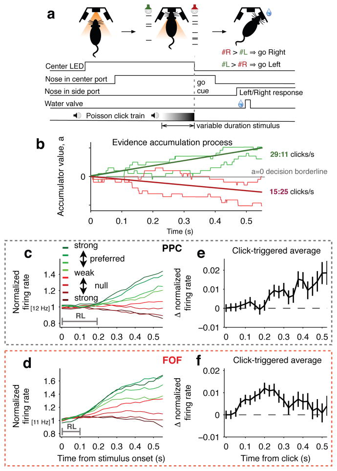
We trained rats on a previously developed decision task in which subjects accumulate sensory evidence over many hundreds of milliseconds to inform a binary left-right choice (“Poisson Clicks” task, Fig. 1a, Extended Data Fig. 1a–c)¹⁰. On each trial, rats kept their nose in a central port during the presentation of two simultaneous trains of randomly-timed auditory clicks, one played from a speaker to their left and the other from a speaker to their right. At the end of the variable-duration stimulus, the rat’s task was to decide which side had played the greater total number of clicks (Fig. 1a). Easy trials had a large mean rate difference between the two click trains (e.g., 39:1 clicks/sec), while difficult trials had a small mean rate difference (e.g., 21:19 clicks/sec). Accumulation of evidence models predict that averaging within a given difficulty class will produce a mean trajectory for the accumulated evidence that gradually ramps over time with a slope proportional to the mean strength of the sensory evidence (Fig. 1b). This type of correlate of evidence accumulation has been reported in several interconnected primate brain regions, including the PPC and frontal eye fields^3–5,7,8,11. To examine whether signatures of evidence accumulation are present in the rodent brain, we recorded from 394 neurons in PPC of 4 rats and 397 neurons in FOF of 6 rats while they performed the Poisson Clicks task. These two areas that have been suggested as potential rat homologues of primate PPC and FEF^12,13. We recorded all isolatable neurons encountered regardless of response properties. Ninety-three neurons in PPC (23%) and 128 neurons in FOF (32%) exhibited firing rates during the pre-movement period (from stimulus onset to center port withdrawal) that were significantly different (p<0.05) for trials that subsequently ended with a right versus a left choice. This pre-movement side selectivity is consistent with previous findings in both rat PPC^14,15 and FOF¹³. We focus on these pre-movement side-selective neurons because they are most likely to play a role in decision formation.

Figure 1. Choice-selective neurons in PPC and FOF exhibit signatures of evidence accumulation.

a, Sequence of events for each trial. b, Schematic of the evidence accumulation process. Each right (left) click provides a single quantum of positive (negative) evidence. The thick green line shows the expected trajectory, averaged over many trials, of the accumulating evidence for a mean stimulus strength of 29:11 clicks/sec. The red line shows this for 15:25 clicks/sec. The lighter-colored traces show how individual trials within a given stimulus-difficulty class meander based on each trial’s variable click times. At the “go” signal (offset of center LED), the sign of a indicates the appropriate decision. c, PPC population responses. Trials were grouped by average strength of the sensory evidence. Green traces correspond to stimuli in the preferred direction of the recorded neurons and red traces to the non-preferred direction. Darker hues correspond to easier trials. Responses exhibit ramping profiles that depend on the mean stimulus strength. The PPC response lag (RL) until stimulus-strength-dependent ramping was ≈200 ms. n = 93 neurons. d, Same as (c) for neurons in the FOF. Similar to PPC, responses exhibit ramping profiles that depend on the mean stimulus strength. RL in the FOF is ≈100 ms. n = 128 neurons. e, Click-triggered average response ± s.e.m. in PPC. f, Same as (e) for FOF.

Side-selective neurons in both PPC and FOF exhibited average firing rates that were initially constant in time and then ramped upwards for stimuli in the preferred direction with a slope proportional to the stimulus strength. A similar but downwards ramping pattern was found for anti-preferred-direction stimuli (Fig. 1c,d; Extended Data Fig. 1d,e for single neuron examples). These response profiles are similar to those found in monkey LIP and FEF during visual motion discrimination tasks^3–5,11, suggesting that rats and monkeys may use similar algorithms and related circuits to perform evidence accumulation.

We extracted the average influence of a single quantum of sensory evidence (a click) on the neural firing rates by computing the click-triggered average firing rate. Individual clicks have a measurable and sustained influence on PPC neural responses (Fig. 1e), consistent with the sustained effects of analogous manipulations in monkey PPC¹⁶. Individual clicks also produced a sustained influence on FOF neural responses, albeit with a magnitude that slowly but significantly decayed over several hundred milliseconds (Fig. 1f). No equivalent experiment from primate FEF exists as yet for comparison. The longer mean latency of the click-triggered average in PPC (~200 ms) compared to FOF (~100 ms) suggests that sensory information in this task may reach the FOF through circuits that bypass the PPC.

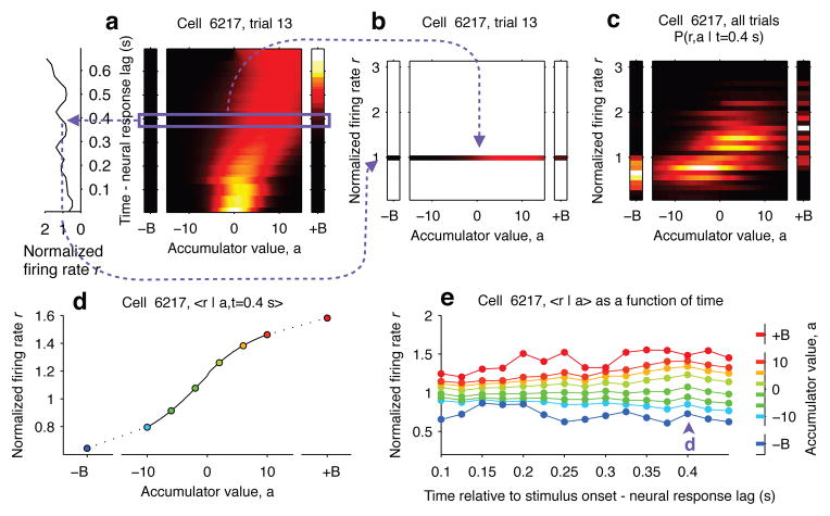
We used the behavioral model previously developed for this task¹⁰ to obtain trial-by-trial, moment-by-moment estimates of the accumulating evidence, denoted by a(t) (Extended Data Fig. 2, Extended Data Table 1). Together with the simultaneously recorded firing rates r(t), this enabled the estimation of “tuning curves” that specify, for each point in time during the stimulus, how r depends on a (Fig. 2).

Figure 2. Computing tuning curves that describe the relationship between neural activity and accumulated evidence.

a, One trial for an example neuron from PPC. The left side shows the neuron’s firing rate, and the right side shows the behavioral model’s estimate of the evolution of the distribution of a (color represents probability density). Time runs vertically and is aligned to stimulus onset minus neural response lag. ±B correspond to the “sticky” decision-commitment bounds on evidence accumulation. b, Building a map of firing rate versus accumulator value. At a given timepoint (here, t=0.4), we copy the distribution of a (purple box) to a vertical position given by the neuron’s firing rate. c, Continuing with the same timepoint, we add a slice from very recorded trial. This produces the full joint distribution P(r,a | t=0.4), the probability of seeing firing rate r and accumulator value a at time t=0.4. d, The accumulator values are binned, and mean firing rate is computed for each bin to generate a neural tuning curve as a function of a. e, The process is repeated for each timepoint. Each vertical slice corresponds to a tuning curve, with the one from panel (d) shown above the purple arrowhead.

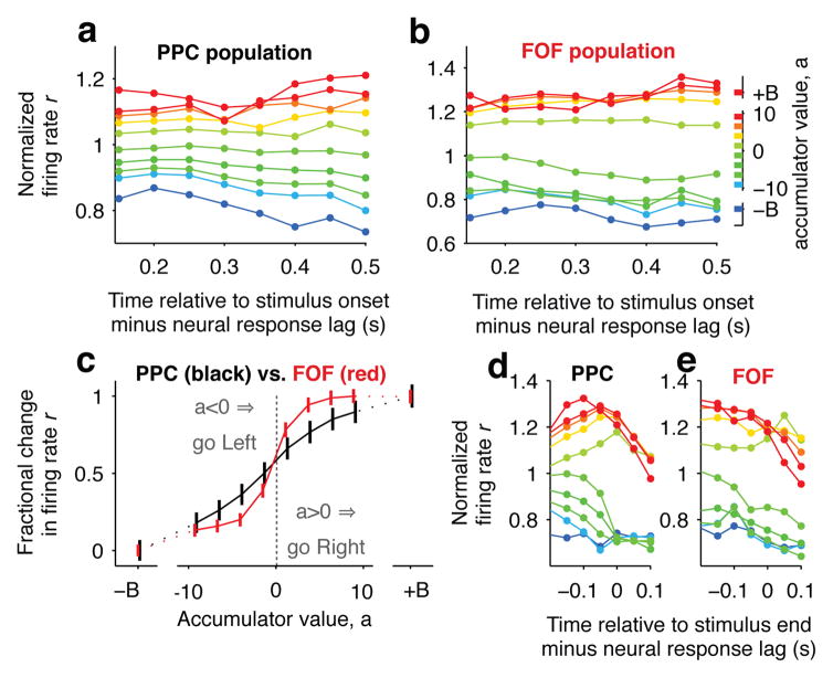
This analysis revealed that PPC encoded the accumulator’s evolving value a(t) using a graded map that is stable across time (Fig. 3a). A similar encoding was observed in monkey PPC, albeit using a task that did not require a temporal accumulation strategy¹⁷. Thus, during decision formation, firing rates in PPC change over time as the accumulated evidence changes, but at any timepoint the graded value of the accumulator is encoded, by a fixed map, into a graded firing rate. In this way, the firing rate provides the answer to the question “what is the value of the mentally accumulated evidence?”

Figure 3. PPC encodes graded accumulated evidence while FOF has a more categorical encoding.

a, Relationship between PPC population firing rate and accumulator value aligned to the stimulus onset minus the neural response lag (200 ms for PPC). Colors indicate accumulator value with ±B corresponding to sticky accumulation bounds. The a → r map in PPC is graded and relatively stable over time. n = 93 neurons. b, Same as (a) for FOF (100 ms neural response lag). The a → r map is again relatively stable over time, but the responses appear to be more clustered based on the sign of a. n = 128 neurons. c, Average ± s.e.m. over the full time period shown (t=0.15 to t=0.5). PPC, in black; FOF, in red. Responses were scaled to span the range from 0 to 1 to account for differences in dynamic range. PPC shows a smoothly graded relationship, while FOF shows a sharper dependence on the sign of the accumulator value. d, Relationship between PPC population and accumulator value aligned to the putative end of the decision process, which is defined as the time relative to the stimulus end minus the response lag.

Despite the similarities between FOF and PPC based on trial-averaged responses (Fig. 1c,d), the tuning curve analysis revealed a very different encoding of the accumulator’s value a(t) in the FOF. Neurons in the FOF exhibited a more categorical mapping between firing rate and the sign of the accumulator value that tended to cluster into an a>0 and an a<0 group, while the mapping was again stable across time (Fig. 3b). The sign of a indicates the choice, so the FOF categorically encodes which of the two available choices is favored by the evidence accumulated so far. Thus, FOF responses can be approximately described as the categorical answer to the question “if the go signal came now, which choice should I make?”

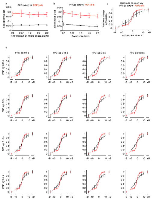
A direct comparison of the time-averaged tuning curves showed a significantly larger slope at the zero-crossing for FOF compared to PPC (Fig. 3c; PPC: 0.058 ± 0.003, FOF: 0.158 ± 0.015, mean ± 95% CI), which indicates a sharper transition of firing rate between negative and positive accumulator values for FOF. This difference was robust to variations in the time constant of integration and the value of a “sticky” decision commitment bound in the behavioral model of evidence accumulation, variations in neural response latencies, and whether the behavioral model was fit individually to each rat or to the aggregate behavior for all rats (Extended Data Fig. 3 and 4). The difference between PPC and FOF was also apparent at the level of individual neurons. We computed the steepness of each neuron’s tuning curve, and while there was overlap between the PPC and the FOF populations, there was a significant shift towards greater steepness for the distribution of FOF neurons compared to PPC neurons (p<0.001, Extended Data Fig. 5). This difference in encoding between PPC and FOF was consistent both with the response profiles (Fig. 1c,d) and the click-triggered average responses, including the diminishing trend for the FOF (Extended Data Fig. 6). The difference in encoding between PPC and FOF was not maintained after the end of the decision process. During the period of motor preparation, the FOF maintained a categorical encoding, while the graded encoding in the PPC converged to a categorical encoding (Fig. 3d,e).

The more categorical encoding found in the FOF suggests that, contrary to current views^3,5,7–9, this brain region may not be involved in the graded evidence accumulation process itself, but rather may be more involved in the conversion to a categorical choice. Such a view predicts that FOF activity should have an impact on behavior only at the end of stimulus presentation, which is when information about the categorical choice will be used to generate a motor response. In contrast, if the FOF were involved in evidence accumulation--a process that occurs throughout the stimulus presentation¹⁰--its activity should have an impact on decision formation throughout the entire sensory stimulus.

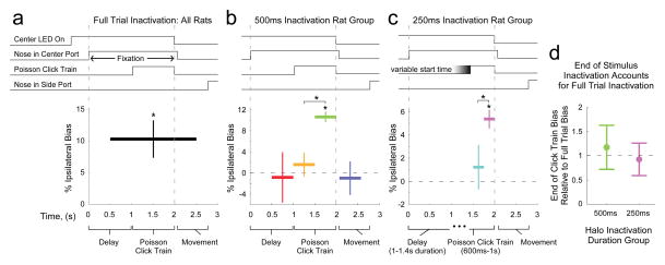
To test these predictions, we used halorhodopsin eNpHR3.0 to unilaterally and transiently inactivate the FOF during the Poisson Clicks task (Extended Data Fig. 7). Full-trial inactivation (2 s period from 500 ms before auditory stimulus onset until 500 ms after stimulus end, Fig. 4a) resulted in a significant ipsilateral choice bias (10.3 ± 3.0%, p<0.01, mean ± SEM across rats). We next assessed the temporal specificity of the effect of FOF inactivation using four different 500-ms time periods: the delay before stimulus onset, the first half of a 1-sec stimulus, the second half of a 1-sec stimulus (“peri-choice”), or the movement period (“post-choice”). Only peri-choice inactivation led to a significant ipsilateral bias (Fig. 4b, 10.6 ± 1.0%, p<0.01). Inactivation during the early accumulation period produced a smaller effect (p<0.01) that was not significantly different from zero (p=0.48). In a second group of rats we used even shorter inactivation periods: either the next-to-last, or the final (“peri-choice”) 250 ms of a variable-duration click train. Again, only the peri-choice perturbation had an effect on behavior (Fig. 4c, 5.4 ± 0.8%, p<0.01), while the effect of perturbation just 250 ms earlier was smaller than the peri-choice effect (p<0.01) and not statistically significant (p=0.45). Furthermore, in both the 500-ms and 250-ms groups of rats, the magnitude of the bias induced by peri-choice inactivation fully explained the magnitude of the bias for full-trial inactivation (Fig. 4d, peri-choice normalized by full-trial bias = 1.17 ± 0.45 and 0.93 ± 0.33 for each group, respectively). Consistent with the idea that the FOF’s dominant role is to control the categorical choice, a model-based analysis indicated that a post-categorization bias explained these optogenetic inactivation data significantly better than alternative forms of bias that directly affected the accumulation process¹⁸ (p < 0.05, see Methods; Extended Data Fig. 8). Finally, and again consistent with the FOF playing a role that is separate from the click accumulation process, we found no correlation between choice biases induced by unilateral perturbation and click counts or stimulus duration (Extended Data Fig. 9).

Figure 4. Temporally-precise transient halorhodopsin-mediated inactivation reveals that FOF activity has a significant impact on decision formation only at the end of the auditory stimulus presentation.

a, b, c, The task structure is shown at the top. For the lower panels, the horizontal extent of the thick black or colored bars indicates the period of inactivation (laser on). The vertical position indicates the average bias across rats induced by the corresponding period of FOF inactivation (% “went ipsi” laser on - “went ipsi” laser off). Asterisks indicate p<0.01 (bootstrap) of effect size or comparison. a, Bias caused by “full-trial” (2 s long laser pulse) inactivation. n = 18 rats. b, Bias caused by 500 ms inactivation during the pre-stimulus period (red; n = 5 rats), the first half of the stimulus (yellow; n = 9), the second half of the stimulus (“peri-choice”, green; n = 9), or the post-stimulus movement (purple; n = 5). c, Bias caused by 250 ms inactivation during the next-to-last 250 ms (light blue; n = 7), or the final 250 ms (“peri-choice”, magenta; n = 7) of a 0.6 to 1.0 s duration stimulus. d, Peri-choice inactivation bias normalized by “full-trial” inactivation bias (500 ms group in green; 250 ms, in magenta). Normalization performed for each rat independently. For all panels, error bars show s.e.m. across rats.

Our results suggest that rather than participating in a single, distributed process during decision-making¹⁹, neurons in parietal and prefrontal areas have distinct relationships to accumulating evidence. PPC neurons veridically encode a graded value of the accumulated evidence, even though separate work from our laboratory suggests that PPC activity is not necessary for choice behavior in this task¹⁸. In contrast, perhaps in readiness for the “go” signal which comes at a variable duration after stimulus onset, neural activity in the FOF can be approximately described as representing, throughout the stimulus, the categorical answer to the question “if the go signal came now, which choice should I make?” Unilateral FOF perturbations affect choice behavior only at the end of the evidence accumulation period, when the provisional choice must be converted into a motor act. These results suggest that accumulation occurs upstream to FOF and call into question the prevailing view that prefrontal cortex is part of the neural circuit for accumulation of evidence^3,5,7,8.

Methods

Subjects

27 male Long-Evans rats (Rattus norvegicus) between the ages of 6 to 24 months were used for this study. 9 rats were used for neural recordings (1 for both PPC and FOF), and 18 rats were used for optogenetic inactivation. All statistical tests were made between groups with similar sample sizes. Investigators were not blinded to experimental groups during data collection or analysis. Animal use procedures were approved by the Princeton University Institutional Animal Care and Use Committee and carried out in accordance with National Institutes of Health standards.

Behavior

Rats were trained to perform an auditory evidence-accumulation decision task¹⁰. For each session, rats were placed in a behavioral training box. At the start of each trial, rats are instructed by a LED to place their nose in a central port and maintain nose fixation. After a delay of at least 0.2 s, they were presented with a train of randomly timed clicks from a left speaker and simultaneously, a different train of clicks from a right speaker. The click trains were generated by Poisson processes with different underlying rates. For neural recording sessions, the duration of stimulus presentation was varied randomly from trial to trial, with durations ranging from 0.1 to 1.2 s. For “full trial” and 500 ms optogenetic inactivation sessions, the stimulus duration was 1 s for all trials. For the 250 ms optogenetic inactivation sessions, the stimulus duration ranged from 0.6 to 1.0 s. When the stimulus ended, the central LED was turned off as a “GO” signal, and rats indicated a choice by making an orienting movement to one of the side nose ports. They were rewarded with a water drop from that port if they chose the side that played more clicks. Trial difficulty was also manipulated by changing the ratio of right to left clicks, with the total mean click rate held fixed at 40 Hz. For neural recording sessions, mean click rate ratios varied from 39:1 clicks/s for the easiest trials to 20:20 clicks/s for the most difficult ones. For optogenetic inactivation sessions, mean click rate ratios varied from 39:1 clicks/s to 26:14 clicks/s. Model-based (Extended Data Table 1) as well as model-free (Extended Data Figure 1) analyses were used to confirm that the rats were basing their decisions on evidence gradually accumulated throughout each stimulus period.

Recordings

Rats were implanted with custom-made microdrives and recordings were made with platinum-iridium tetrodes, as described previously¹³. FOF recording sites were centered at +2 AP, ± 1.3 ML (mm from Bregma); PPC sites were centered at −3.8 to −4.1 AP and ± 2.2 ML. The choice of recording area in each particular rat was assigned randomly. Electrode placements were confirmed with histology.

Neural Data Analysis

Action potentials were isolated as belonging to single neurons by performing manual cluster cutting of tetrode waveforms from events that exceeded a threshold level on any of the tetrode channels. We recorded spike times for all isolatable neurons encountered regardless of response properties. We then selected for further analysis those neurons that had a mean response at stimulus onset larger than 1 Hz and significantly different firing rates during the pre-movement period for trials that subsequently end in right vs. left choices (p<0.05, Receiver operating characteristic). The “pre-movement period” was defined to start at stimulus onset and end at response initiation. We defined the choice side that yielded the larger response as the preferred side. The preferred side was contralateral for 59.1% of the PPC neurons and 59.4% of the FOF neurons. We note that mixed selectivity like this in rat prefrontal cortex still yields ipsilateral biases after unilateral inactivation^13,20.

Individual trial rate functions were generated by smoothing the spike trains with a half-gaussian filter with 0.1 s standard deviation. Before combining responses into a population average, responses were normalized by the mean response for each neuron at stimulus onset. To generate peri-event time histograms (PETHs), responses were sorted for each cell by the mean stimulus strength. Mean stimulus strength was defined by dividing trials for each cell into 8 quantiles based on preferred minus non-preferred click rates--that is, the difference in the number of clicks presented divided by the stimulus duration. More precisely, positive and negative click rate trials (those with more preferred and non-preferred clicks, respectively) were separately sorted into 4 quantiles each. Trials with the same number of preferred and non-preferred clicks were assigned in equal numbers to the two quantile bins with lowest absolute magnitude rates--that is, those closest to zero. For all analyses aligned to stimulus onset, trials were included only up to the time of movement onset.

To measure the effects of single clicks on neural responses, “click-triggered averages” were calculated as follows. For each neuron, we first grouped the trials based on the underlying Poisson rates used to generate the stimuli. For each group, we calculated the mean PETH, which corresponds to the expected neural response at each point in time for each Poisson rate group. We subtracted this mean response from each member (trial) in the group to yield the residual response with respect to the expectation given the Poisson rate. Due to the Poisson nature of the stimulus, given an underlying click-generating Poisson rate, the presence of a click at one moment in time has no bearing on the probability of a click at other times. Therefore, if one aligns the residual response to a click, it describes the change in response associated with that click relative to the average expected response to clicks at other times. In this way, the residual response allowed us to isolate the effect of a single click apart from the confounding effect of the mean response across time for a given Poisson rate. Thus, we aligned the residual responses to the time of each click and averaged across these alignments to obtain the “click-triggered average” response across all clicks for each Poisson rate group; the click-triggered average for each neuron was the result of averaging across groups. To combine across both preferred-direction and non-preferred-direction clicks, the residual responses for non-preferred-direction clicks were inverted in sign before averaging.

To make model-based predictions for the click-triggered average, we used the model to simulate evidence accumulation trajectories for 5000 trials based on the same range of stimulus difficulties and durations used to collect neural data. We then encoded these trajectories with either a graded, linear scheme (veridical encoding of accumulated evidence, firing rate r = k₁*a(t) + k₂, where k₁ and k₂ are constants) or a categorical scheme (firing rate r = k₁*sign(a(t)) + k₂, where k₁ and k₂ are constants). For the graded scheme, we introduced an encoding lag with a mean of 0.2 s to match the response lag of PPC. For the categorical scheme, we introduced an encoding lag with a mean of 0.1 s to match the response lag of FOF. For both schemes, the encoding lag was taken from a Gaussian distribution with 0.02 s standard deviation to account for variability in lag across neurons. We then used the same methods described above to measure the click-triggered average of these two encodings.

We used a similar approach to calculate the expected PETH response profiles that would be obtained for a categorical-encoding model (Extended Data Figure 6). To do this, we simply averaged responses from the categorical-encoding model across trials, sorting based on mean stimulus strength with the same method as described above for Figure 1.

Behavioral Model-Based Analysis of Neural Data

To generate tuning curves that specify the relationship between neural firing rates and mentally accumulated evidence, we exploited a trial-by-trial behavioral model of the evidence accumulation decision process (Extended Data Figure 2)¹⁰. The model converts each trial’s incoming stream of discrete left and right click stimuli into a scalar quantity a(t) that represents the gradually accumulating difference between the two streams and drives choices: at the end of the stimulus, if a is positive (negative), the model prescribes “choose Right” (“choose Left”). The rat’s behavior is used to fit parameters that govern how a(t) evolves. These parameters quantify sensory and accumulator noise, leakiness/instability of the accumulation process, a sticky accumulation bound, sensory depression/facilitation, side bias, and a lapse rate which corresponds to a fraction of trials on which a random choice is made. Quantifying and taking into account the noise sources implies that on each trial, the model estimates the evolution of a noise-induced probability distribution over values of the scalar a(t). Note that in addition to the probability distribution over a(t), each trial also has an associated lapse probability, which is constant as a function of time. At any moment of time, the forward version of the model allows for the estimation of the distribution of the accumulated evidence given the stimulus that was presented. A better estimate of the accumulated evidence can be obtained by also taking into account the choice made at the end of the trial. This is calculated using the backward propagation of accumulator values that are consistent with that choice at the end of the stimulus presentation (Extended Data Figure 2b)¹⁰. We use this improved estimate that also takes into account subject’s choice to relate the accumulator value to neural responses.

For the analyses presented in the main text, the behavioral model was fit separately to each rat (see model parameters, Extended Data Table 1). Thus, in estimating the value of a(t), variability between individual rats was taken into account. To ensure that this variability did not itself result in important effect differences, we also performed separate analyses where we estimated a(t) from a single set of model parameters derived from the combined behavior across all rats (Extended Data Figure 4).

In addition to these estimates of a(t), we also have an estimate of each neuron’s response as a function of time from the single trial rate functions described above. The estimates of the neural response and accumulated evidence were then used to calculate the joint probability distribution between those two variables as a function of time for each neuron. The correspondence between time in the model and neural time was determined based on the latency of the stimulus-dependent responses in each region. Thus, t = 0 in the model was taken as 200 ms after stimulus onset for PPC and as 100 ms for FOF. From the joint probability, we extracted the neuron’s response given the value of the accumulator. We combined across neurons by weighting the contribution of each by the inverse of the variance of this conditional distribution. This gives more weight to representations that are less noisy.

To quantify the relationship between neural response and accumulator value, we first averaged across the time period from 0.15 to 0.5 s into the decision process (Fig. 3c). To account for the variety of dynamic ranges of the neural responses, we scaled the responses to span the range from 0 to 1, either for individual neurons (Extended Data Figure 5a) or for each cortical region (Fig. 3). We then fit the relationship of the response to the accumulator with a four-parameter sigmoid with the following equation:

$$r=k_1+\frac{k_2}{1+e^{-k_3(n-k_4)}}$$

In this equation, k₂k₃/4 determines the slope at zero-crossing, which characterizes whether the neural response changes smoothly between negative and positive accumulator values or whether it changes sharply in this region. We extracted this parameter and its confidence interval for the both the PPC and FOF populations. Statistical comparisons between the populations were calculated using nonparametric bootstrap procedures resampling from the populations of neurons with replacement. We also extracted the shape parameter for individual neurons and used the nonparametric Mann-Whitney U (rank sum) test to determine if the medians of each population distribution were significantly different.

We also performed a number of analyses to ascertain to what extent specific parameter values were critical for our results. We focussed on the time constant of accumulation and the sticky decision bounds, because these two parameters describe the extent to which psychophysical accumulation differs from optimality. For both parameters, we scaled its best-fit value by factors of 0.5, 0.67, 1.5, and 2, and compared the slopes of the tuning curves for PPC and FOF based on the revised estimates of a(t) using these scaled parameters (Extended Data Figure 3a,b). We also tested whether different neural response lags would affect the results. To do this, we compared neural tuning curves for PPC and FOF while varying the latency between auditory clicks and neural representation for each area using a range from 0.1 s to 0.25 s. This results in a matrix of comparisons, where response lag for PPC varies along one axis and response lag for FOF varies along the other axis (Extended Data Figure 3d).

Optical Fiber Chemical Sharpening

Modifying previously published protocols²¹, we began construction with a standard off the shelf 50/125 μm FC-FC duplex fiber cable (FiberCables.com). The cable jacket, strengthening fibers, and outer plastic coating (typically white or orange) were fully removed leaving 1 cm of fiber optic cable and inner plastic coating (typically clear) intact. 2 mm of the fiber tip (with final layer of plastic coating still attached) was submerged in 48% hydrofluoric acid topped with mineral oil for 85 minutes, followed by water for 5 minutes (submerging 5 mm), and acetone for 2 minutes (to soften the plastic). The plastic coating was then gently cut with a razor and pulled off with tweezers to reveal a 1 mm sharp etched fiber tip. Enough plastic was removed, depending on the depth of the targeted site, to ensure that only the glass fiber optic would be inserted into the brain.

Optogenetic Virus Injection and Fiber Implantation

For optogenetic perturbation experiments, the general surgery techniques follow previous reports¹³. Here we describe the techniques that were unique for this experiment. For viral injection, 2 μl of AAV virus (AAV5-CaMKIIα-eNpHR3.0-eYFP²²) was lightly dyed with fast green powder and front loaded into a glass pipette mounted to a Nanoject (Drummond Scientific) prefilled with mineral oil. The pipette tip was manually cut to ≈ 30 μm diameter. Five closely spaced injection tracts were used with each animal. For the central injection tract, two injections of 9.2 nl were made every 100 μm in depth starting 200 μm below brain surface for FOF for 1.5 mm. Four additional injection tracts were completed, using procedures identical to the central tract, one 500 μm anterior, posterior, medial, and lateral from the central tract. Each injection was followed by a 10 s pause, with 1 minute following the final injection in a tract before the pipette was removed. A total of 1.5 μl of virus was injected over a 30 minute period consisting of ≈ 160 separate injections. A chemically-sharpened fiber optic (50 μm core, 125 μm cladding) was then lowered down the central injection tract to a depth of 1 mm. The craniotomy was filled with kwik-sil (World Precision Instruments), allowed to set for 10 minutes, and the fiber optic was secured to the skull with C&B Metabond and dental acrylic. After surgery, the primary incision was closed with sutures which allowed only the FC connector to protrude. Halorhodopsin expression was allowed to develop for 6 weeks before behavioral testing began.

Optogenetic Pertubation

The animal’s implant was connected to a 1 m patch cable connected to a single fiber rotary joint (Princetel) mounted on the ceiling of the behavioral chamber. This was connected to a 200 mW, 532 nm laser (OEM Laser Systems) operating at 25 mW which was triggered with a 5 V TTL. Laser illumination occurred on a random 25% of trials. Behavioral bias was measured as the mean difference between the observed “go ipsi” rate for inactivation and control trials for each of 10 binned stimulus strengths. Thus, a positive value represents an increase in ipsilateral responses on laser illumination trials. Confidence intervals and statistical comparisons for this bias parameter were calculated using nonparametric bootstrap procedures resampling from the population of rats with replacement. All rats were included in the analysis of full-trial inactivation. However, two rats were not included in the higher temporal resolution optogenetic experiments because they did not exhibit significant full-trial effects. The 500 ms and 250 ms experiments were performed sequentially in different groups of rats. Therefore, the assignment of group was not randomized.

Measurement of Optogenetic Inactivation

To measure the effects of optogenetic inactivation, both acute and chronic neural recordings were performed during optogenetic inactivation. For the acute recordings, a sharp etched fiber optic and sharp tungsten electrode (0.5 or 1.0 M^) were independently advanced into the cortex of an anesthetized rat. The fiber was positioned in the center of the field of infection at a given depth. Every location that yielded regular spiking activity of ~5 Hz or greater (single and multi unit activity) was tested 10 times with 500 ms periods of laser illumination at 25 mW every 5 s. For chronic recordings, a silicon probe array (A4x8-5mm-200-400-177, NeuroNexus) was lowered 1.8 mm into cortex. The probes were oriented in the medial-lateral dimension, centered at 1.3 mm medial and 2.25 mm anterior from bregma (0.25 mm anterior from the central injection tract). The optical fiber tip was lowered in at a 30 degree angle with the final tip position located 1 mm from the brain surface, 2 mm anterior and 1.3 mm medial from bregma. Laser illumination was identical to that used as for other awake behaving rats.

Analysis of optogenetic effects using behavioral model

We used the trial-by-trial behavioral model described previously (Extended Data Figure 2) to better understand the cause of the ipsilateral bias induced by unilateral FOF inactivation (Fig. 4a–c). The original model had only one parameter to describe a right versus left choice bias, the decision borderline Þ. We adapted the model, adding several parameters that could describe possible sources of a side bias, and asked which of these variants best fit the rats’ behavior during trials in which the FOF was unilaterally inactivated. The 4 different sources of a choice bias that we considered were:

1. “Post-categorization bias”. The model’s distribution of values of the accumulator a at the end of the stimulus is categorized into “Go Right” versus “Go Left” choices according to a > Þ versus a < Þ, where Þ is the decision borderline parameter. When performing unilateral inactivation, the choice directions can be mapped as “contralateral” or “ipsilateral” with respect to the side of inactivation. We defined “post-categorization bias” as a process that takes a fraction of the trials categorized as choices contralateral to the inactivated side of the brain, and converts them into ipsilateral choices. The fraction of trials thus converted is a free parameter, fit to the behavioral data (from unilateral FOF inactivation trials).

2. “Accumulator shift”. This is an additive bias that alters the the final value of the accumulator. It is mathematically equivalent to altering the value of the decision borderline Þ that categorizes accumulator values into right and left choices (or, contralateral and ipsilateral when considering the choice with respect to the side of unilateral inactivation). In the behavioral model, this is implemented by changing a to a + shift after the end of accumulation but before the application of the decision borderline, or (equivalently) by changing the decision borderline Þ to Þ - shift, with shift being the free parameter, fit to the behavioral data from unilateral FOF inactivation trials.

   Because the FOF has been suggested as analogous or even homologous to the primate FEF^13,23–25, and the primate FEF is known to be involved in spatial attention²⁶, we considered two possible ways in which an effect that could be interpreted as unbalanced spatial attention might bias sensory input signals during the task:

3. “Unbalanced input gain”. In the unperturbed case unadapted right and left clicks both have the same impact magnitude on the accumulator a (+1 and −1 for right and left clicks respectively, before accounting for click adaptation). We considered the possibility that the clicks from the two sides could have different impact magnitudes. Such an unbalanced input gain was implemented by allowing the contralateral click magnitude to be a free parameter (while preserving its sign), and this free parameter was fit to the behavioral data from unilateral FOF inactivation trials.

4. “Unbalanced input noise”. In the unperturbed case unadapted right and left clicks both contribute the same amount of variance to the accumulator a. Thus both right and left click streams have the same signal-to-noise ratio (SNR). Here we considered varying the SNR of one side by altering the variance contributed to the accumulation by ipsilateral versus contralateral clicks. The unbalanced input noise was implemented by allowing the contralateral noise variance to be a free parameter, fit to the behavioral data from unilateral FOF inactivation trials.

We note that (3) and (4), unbalanced input gain and and unbalanced input noise, both imply mechanisms that act throughout the entirety of the accumulation process. In contrast, (1) and (2), the post-categorization bias and the accumulator shift, can be implemented via a mechanism that acts only at the end of the accumulation process.

We compared how well these possible sources of bias in the behavioral model could account for the trial-by-trial choice behavior during both full-trial and peri-choice FOF inactivation. For the full-trial inactivation, we considered all four alternative implementations described above. For the peri-choice inactivation, we considered the two alternatives that predict an effect on behavior only during the end of the stimulus presentation period, namely (1) and (2), the post-categorization bias and the accumulator shift. In both the full-trial and peri-choice inactivation cases, we began by fitting the control non-inactivation trials with the standard model described in Extended Data Figure 2, combining data across all rats used in each type of experiment. These control non-inactivation trials comprised 75% of the total trials and were randomly interleaved with the inactivation trials within the same behavioral sessions. Starting from the parameters that best fit behavior on these control trials, we then examined how well each single-parameter implementation of bias under consideration could fit the inactivation data. In all cases, we report both the overall log-likelihood of the fit, and how well, on average, each alternative source of bias predicts the response on each trial. We illustrate the fits across multiple trials by comparing the psychometric functions produced by the different models to those found in the data. We performed statistical comparisons of the quality of the fits using a nonparametric resampling bootstrap procedure. We first generated 200 sets of trials with the same trial count as the original data by resampling the original data with replacement. We then fit each of these sets with the models described above and measured the difference in likelihood between post-categorization bias and the other alternatives for each resampled set of data. This provided a distribution of likelihood ratios from which we could estimate the statistical probability that post-categorization bias provides an improved fit compared to the other models.

Extended Data

Extended Data Figure 1. Rat behavior and example neurons.

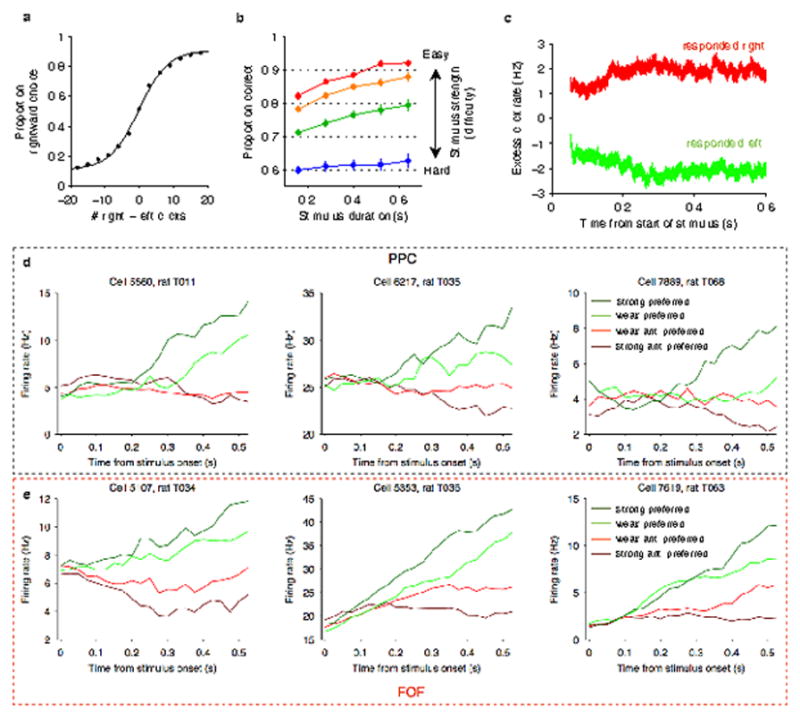
a, Mean psychometric function across all rats. Accuracy was highest for the largest click differences (the left and right endpoints of the curve) and lower for smaller click differences (the middle of the curve). b, Mean chronometric function across all rats. Trials were sorted by binned stimulus strength (difficulty), with mean click ratios ranging from 39:1 clicks/s for the easiest trials to 25:15 clicks/s for the hardest trials. In general, accuracy improved with longer stimulus durations. c, Mean psychophysical reverse correlation across all rats. This was calculated based on trials with minimum duration of at least 0.6 s. For each timepoint in each trial, we first computed the excess click rate difference (right - left clicks/s) relative to the value expected given the random processes used to generate the trial. These excess click rates were averaged separately for trials ending with a right choice (red) and for trials ending with a left choice (green). The separation between the two traces indicates how strongly clicks from the corresponding timepoint influence the final decision. d, Peri-event time histograms (PETHs) aligned to stimulus onset were calculated for 3 example PPC neurons. Trials were sorted into 4 stimulus strength bins for each neuron. Green traces correspond to the preferred-direction stimuli and red traces correspond to anti-preferred-direction stimuli. Darker colors correspond to stronger stimuli (less difficult) and brighter colors correspond to weaker stimuli (more difficult). e, PETHs for 3 example FOF neurons using the same conventions. In both regions, individual neurons exhibit ramping activity that depends on stimulus strength.

Extended Data Figure 2. Behavioral model, following Brunton et al. (2013).

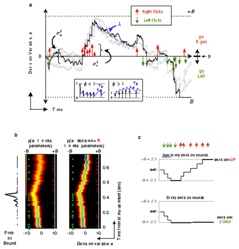
a, At each timepoint, the accumulator a (black trace) represents an estimate of the “Right” vs “Left” evidence accrued so far. At stimulus end, the model decides “Right” if a > Þ (the decision borderline) and “Left” otherwise, where Þ is a free parameter. Light grey traces indicate alternate runs with different instantiations of model noise. These example trajectories are for illustrative purposes; the model estimates the full probability distribution of a at each timepoint.

Right (Left ) clicks change the value of a by positive (negative) impulses of magnitude C.

${\sigma }_a^2$ is a diffusion constant, parameterizing noise in a.

${\sigma }_s^2$parameterizes noise associated with each click.

λ parameterizes consistent drift in the decision variable a. In the “leaky” case (λ < 0, illustrated), drift is towards a = 0, and later clicks impact the decision more than earlier clicks. In the “unstable” case (λ > 0), drift is away from a =0, and earlier clicks impact the decision more than later clicks. The time constant of the accumulation process is τ = 1/λ.

B is the height of “sticky” decision bounds. If a reaches either bound, it leads to decision commitment before the end of the stimulus and later clicks have no impact on the choice.

ϕ, τ_ϕ parameterize sensory adaptation by defining the dynamics of C. Immediately after a click, the magnitude C is multiplied by ϕ. C then recovers towards an unadapted value of 1 with time constant τ_ϕ. Facilitation thus corresponds to ϕ > 1, while depression corresponds to ϕ < 1.

These properties are implemented by the following equations:

if |a| B then da/dt = 0; else

$$da={\sigma }_{a}dW+({\delta }_{t,t_R}·{\eta }_R·C-{\delta }_{t,t_L}·{\eta }_L·C)dt+\lambda \mathit{adt}$$

where

• δ_t,tR,L are delta functions at the times of the auditory clicks.
• η are i.i.d. gaussian variables drawn from N(1,σ_s).
• dW is a white-noise Wiener process.
• Adaptation dynamics are given by:

  $$\frac{dC}{dt}=\frac{1-C}{{\tau }_{\varphi }}+(\varphi -1)C({\delta }_{t,t_R}+{\delta }_{t,t_L})$$

In addition, a lapse rate parameterizes the fraction of trials on which a random response is made.

b, The behavioral model provides an estimate of the evolution of the distribution of a for each trial, with color representing probability density for both panels. The forward version of the model (left panel) estimates the distribution of a at each timepoint based entirely on the click times and model parameters. Leftward (green) clicks push the distribution more negative and rightward (red) clicks push it more positive. The final value obtained by a at the end of the trial dictates the choice. In this example, the distribution of the final value of a is more heavily weighted towards negative values because there were more leftward than rightward clicks for this trial. A better estimate of the distribution of a can be obtained by also taking into account the subject’s choice made at the end of the trial (right panel). The final choice constrains the distribution of a at the final timepoint to have all its mass to one side of the decision boundary (in this example trial, despite the many leftward clicks, the subject chose right, and thus at the final timepoint, all the probability mass is at a>0). This constraint is then propagated backwards in time, to obtain the distribution of accumulator values at each timepoint that is consistent both with the stimulus clicks and the subject’s final choice. The final result is an estimate of the distribution of a at each timepoint that takes into account the click times, the model parameters, and the subject’s choice.

c, Illustration of non-sticky versus sticky decision bounds. Upper panel: response of an accumulator to a sequence of downward (green arrows) and upward (red arrows) impulses when the bound parameter B is 2.5 and the bounds are not sticky. The fourth downward arrow (green) has no impact, because the bounds have been reached, and a cannot go beyond them. But subsequent upward arrows (red) do have an impact, because they do not push against the bounds. Lower panel: response of an accumulator with the same parameters, receiving the same sequence of impulses, but when the bounds are sticky. Impulses subsequent to reaching the bound have no effect. We fit our rats’ behavior data to this non-sticky bound model. We found that, similar to the version with the sticky bounds, the accumulation time constants were long (|τ|=1/|λ|= 1.0 ± 0.2 s, mean ± SEM across rats), and the bounds were high (17.1 ± 2.2, mean ± SEM across rats). Such high bounds once again indicate that the bounds have minimal impact (consistent with this, the difference between the sticky and non-sticky bound models turned out to be negligible).

Extended Data Figure 3. Robustness of distinction between PPC and FOF to parameter variation.

a, The distinction between PPC and FOF encoding is robust to variation of the model’s time constant of integration. The slope of the tuning curves, drawn from the same analysis as Figure 3c in the main text, except that here the analysis was carried out at a variety of integration time constants b, Same analysis performed for a variety of heights for the sticky decision-commitment bounds. In both cases, the corresponding best-fit parameter was scaled by the factor shown on the horizontal axis, and the slope of tuning curve for FOF (in red) vs. PPC (in black) was plotted as a function of that scale factor. Error bars show 95% confidence intervals. The slope of the FOF tuning curve is significantly sharper than the slope of the PPC tuning curve across the entire range of parameter values tested (p < 0.05). c, Tuning curve comparison between PPC and FOF with subset of PPC neurons selected such that the two regions have matched side selectivity. This resulted in n = 50 neurons for PPC and the original n = 128 neurons for FOF. The tuning curve is significantly steeper for FOF (p < 0.05). d, The same analysis as Figure 3c in the main text, except that here we varied the latency applied between click time and neural representation (see Methods). While we would expect that an improper choice of latency would degrade the quality of the estimate of the accumulator value, the slope at the zero-crossing was still significantly larger for FOF compared to PPC for all comparisons (p<0.05).

Extended Data Figure 4. Tuning curves based on model fit to aggregate rat behavior.

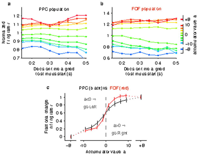
The same analysis as Figure 3 in the main text, except that rather than fitting the behavioral model on a rat-by-rat basis, it was fit to the aggregate behavior of all rats. Thus, all rats share identical model parameter values for this figure. While we would expect that to degrade the quality of the estimate of the accumulator value, the slope at the zero-crossing was still significantly larger for FOF compared to PPC (PPC slope = 0.079 ± 0.004, FOF slope = 0.135 ± 0.026, mean ± 95% CI).

Extended Data Figure 5. Individual neuron analyses.

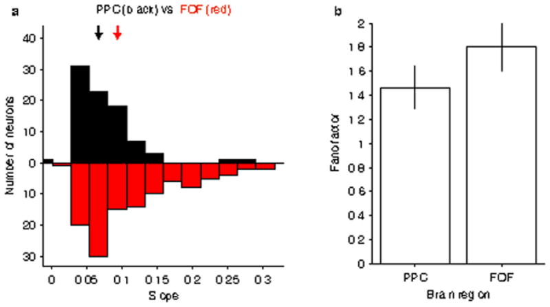
a, The mapping between firing rate and accumulator value is shifted towards steeper slopes for the distribution of FOF neurons compared to the distribution of PPC neurons. Bars show the histogram of individual neuron slopes obtained from a sigmoidal fit of the relationship between firing rate and accumulator value, averaging across time from 0.15 to 0.5 s. Black bars correspond to PPC and red bars correspond to FOF. The arrows indicate the medians of the two distributions. While there is considerable overlap between the two populations, there is a significant shift towards greater steepness for the distribution of FOF neurons compared to PPC neurons (p<0.001, rank sum test). A larger slope corresponds to a steeper change from low to high firing rates at the transition between negative and positive accumulator values. Thus, a steeper slope is associated with a more categorical as opposed to graded encoding of the accumulating evidence. b, To compare neural variability, we measured the fano factor for each neuron as a function of the accumulated evidence and compared across regions. There was not a significant difference in neural variability for the representations in the two areas (p = 0.23).

Extended Data Figure 6. Expected response profiles and click-triggered averages based on graded and categorical encodings.

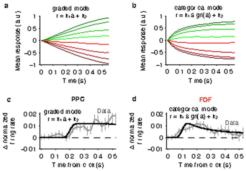
a, Using stimuli corresponding to what was presented to the rats, individual trial responses r(t) were calculated based on the graded encoding r(t) = r = k₁a(t)+k₂, where a(t) is the decision variable obtained from the behavioral model. Then, responses were averaged across trials sorting based on mean stimulus strength with the same exact method as described for Figure 1. b, Same as (a) for a categorical encoding r(t) = k₁sign(a(t))+k₂. The ratio of the positive-to-negative encoding changes over time for each condition, leading to a ramping response profile. This highlights the point that ramping response profiles alone are not a sufficient demonstration of a gradual accumulation process. c, The black line shows the model prediction for the click-triggered average based on a graded encoding of accumulated evidence (r = k₁a+k₂) with a 0.2 s mean encoding lag to match the response lag of PPC. The gray line shows the data from Fig. 1. d, Same as (c) for a categorical encoding of accumulated evidence (r = k₁sign(a)+k₂) with a 0.1 s mean encoding lag to match the response lag of FOF. For both schemes, the encoding lag was taken from a Gaussian distribution with a 0.02 s standard deviation to account for variability in lag across neurons.

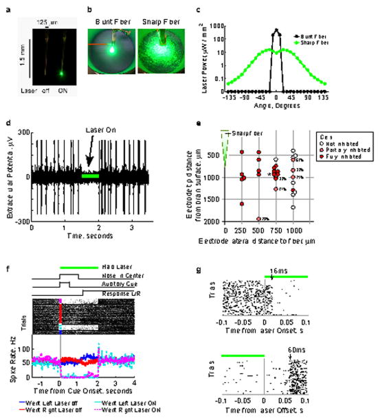
Extended Data Figure 7. Chemically sharpened fiber optics allow extensive inhibition during acute and chronic recordings from cortical regions expressing eNpHR3.0.

a, Image of a chemically sharpened 50 μm core, 125 μm cladding fiber. b, Light spot produced by a blunt and sharpened fiber 2 cm above the floor of a cylindrical container 10.5 cm in diameter. c, Laser power output from a blunt and sharpened fiber as a function of angle relative to the fiber optic tip. 25 mW input power. Power meter was 2.86 mm from the fiber tip. d, Single trace of an acute recording of spontaneous activity in anesthetized primary somatosensory cortex (S1, 1.5 mm posterior, 2.8 mm lateral from Bregma) expressing eNpHR3.0. Laser illumination period, 500 ms, marked by the green bar. e, Location of acute recording units (single and multi) in anesthetized S1 relative to fiber tip and cortical surface. The level of inhibition was measured from ten repeated 500 ms laser illumination periods, delivered every 5 s. Percent reduction displayed next to partially inhibited units. Unit in d indicated with an asterisk. f, Example multiunit activity from the FOF of a rat performing a memory guided orienting task. 2 s laser illumination period initiated at cue onset, resulted in 97% inhibition of spiking activity for both trials where the rat made left or made right responses. g, Multiunit spiking activity (from f) aligned to laser onset (top) and laser offset (bottom). Spiking activity is strongly inhibited ~16 ms following laser onset and recovers ~60 ms following laser offset.

Extended Data Figure 8. Model-based analysis of halorhodopsin mediated inactivation of the FOF, following Erlich et al. (submitted).

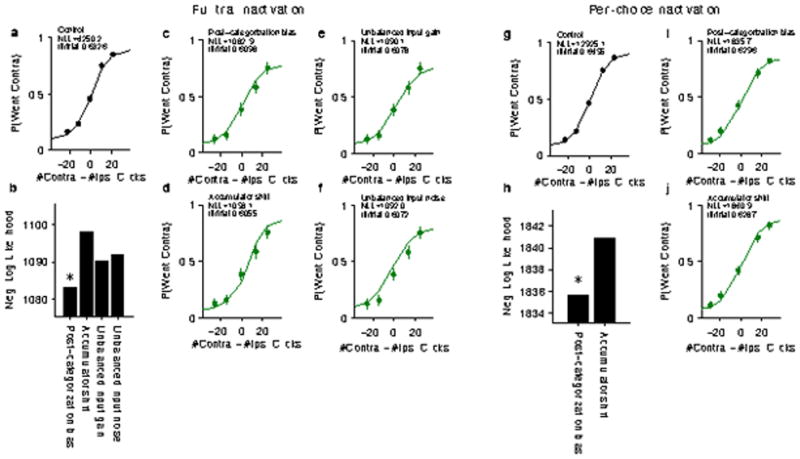
a–f, Full-trial inactivation (figure 4a of main text). a, Control trials with no inactivation taken from sessions with full-trial, 2 s, halorhodopsin inactivation. “Contra” and “Ipsi” sides are relative to the side of the FOF that was inactivated on non-control trials. The curve shows the psychometric function predicted by the best-fit behavioral model based on the same stimuli that produced the behavior. b, Comparison of the negative log likelihood for each candidate source of bias (see Methods). Smaller values correspond to a better fit. The post-categorization bias was significantly better than all other alternatives (p < 0.05, bootstrap). c–f, Data points show the proportion of contralateral choices for full-trial, 2 s inactivation of FOF. The curves show choice behavior predicted by each alternative implementation of choice bias. b, Post-categorization bias. c, Accumulator shift. d, Unbalanced input gain. e, Unbalanced input noise. g–j, Peri-choice inactivation (figure 4b–d of main text). g, Control trials with no inactivation taken from sessions with either 500 ms or 250 ms peri-choice inactivation. The curve shows the psychometric function predicted by the best-fit behavioral model based on the same stimuli that produced the behavior. h, Comparison of the negative log likelihood for both sources of bias. Smaller values correspond to a better fit. The post-categorization bias was significantly better than the accumulator bias (p < 0.05, bootstrap). i–j, Data points show the proportion of contralateral choices for peri-choice inactivation of FOF. The curves show choice behavior predicted by the two versions of bias that predict an effect only at the end of the stimulus period. i, Post-categorization bias. j, Accumulator shift.

Extended Data Figure 9. FOF inactivation induced response bias does not correlate with click count or click train duration.

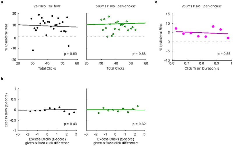
This figure shows further analysis of the data from Fig. 4 of the main text. a–b, During both the full-trial and 500 ms peri-choice inactivation sessions 50% of the trials had the click train duration fixed at 1 second (half inactivation half control trials). The remaining 50% were non-inactivation control trials with stimulus durations that varied randomly (not included in this analysis). All trial types were randomly interleaved. The Poisson nature of the click stimuli means that the number of clicks varied from trial to trial even for trials with the same duration and net click difference. a, We first asked whether the magnitude of the ipsilateral bias was correlated with the number of clicks for these fixed duration trials, and found that it was not (p=0.80 and p=0.88, for full trial and 500 ms peri-choice inactivations, respectively). b, In a separate analysis we asked if given a fixed click difference, if more clicks leads to an excess bias. We first separated trials into groups with equivalent click differences (ipsi count - contra count). Each trial’s actual click count was then subtracted by its group mean and normalized by its group standard deviation. This gives the z-score of the excess clicks on each trial given that trial’s click difference. We repeated this z-score normalization for the response bias on each trial (1 for respond ipsi, 0 for respond contra, bias = response on an inactivation trial - mean response on equivalent non-inactivation control trials). This gives a plot of the excess bias as a function of excess clicks. We found no significant correlation (p = 0.43 and p = 0.32 for full trial and 500 ms peri-choice inactivations, respectively). c, In the 250-ms inactivation experiment, click train durations varied both for control and inactivation trials. Here we asked whether the induced bias was correlated with the variable click train duration, and again found that it was not (p=0.66).

Extended Data Table 1.

Best fit parameters of behavioral model.

Experiment	Data set	λ	${\sigma }_a^2$	${\sigma }_s^2$	B	ϕ	τϕ	Þ	lapse	full trial
PPC recordings	B053	1 51	0 0	23 3	15 0	0 39	0 07	0 02	0 07	0 47
PPC recordings	T011	1 44	0 0	61 8	19 9	0 45	0 02	−0 58	0 05	0 40
PPC recordings	T035	−1 61	24 6	178 7	26 2	0 32	0 03	−0 15	0 05	0 58
PPC/FOF recordings	T068	2 45	0 0	57 5	11 6	0 36	0 04	0 99	0 11	0 46
FOF recordings	B068	2 17	0 0	16 0	16 8	0 41	0 17	0 14	0 10	0 57
FOF recordings	T030	0 46	1 01	39 0	14 5	0 32	0 03	0 20	0 04	0 38
FOF recordings	T034	−0 99	49 7	10 6	17 2	0 58	0 07	−0 69	0 20	0 55
FOF recordings	T036	0 84	0 0	34 1	14 6	0 51	0 07	−0 62	0 11	0 48
FOF recordings	T063	0 42	2 5	139 3	19 6	0 43	0 03	0 09	0 01	0 51
PPC/FOF recordings	physiology combined rat	0 47	0 0	61 3	19 2	0 56	0 06	−0 13	0 09	0 49
FOF optogenetics	B108	0 44	0 1	52 3	17 3	0 10	0 04	−0 57	0 19	0 50
FOF optogenetics	B116	−0 14	54 6	42 5	30 5	0 39	0 05	0 01	0 04	0 47
FOF optogenetics	B117	−2 08	66 0	199 8	31 6	0 48	0 01	0 06	0 00	0 50
FOF optogenetics	B119	−1 65	116 3	88 9	10 2	0 36	0 02	−0 57	0 11	0 54
FOF optogenetics	B120	0 62	0 0	138 4	31 8	0 94	0 50	0 10	0 00	0 42
FOF optogenetics	B123	−1 88	7 0	99 3	31 7	0 54	0 04	−0 58	0 07	0 46
FOF optogenetics	B124	−1 11	0 0	131 3	28 0	0 61	0 03	0 87	0 05	0 44
FOF optogenetics	B125	−0 71	74 4	90 9	11 2	0 30	0 02	−0 02	0 02	0 47
FOF optogenetics	B126	−0 34	0 0	111 0	27 0	0 93	0 50	−0 11	0 00	0 40
FOF optogenetics	B129	0 79	16 5	6 2	15 6	0 29	0 06	0 11	0 05	0 37
FOF optogenetics	K145	0 64	27 6	49 3	13 5	0 45	0 06	−0 26	0 18	0 51
FOF optogenetics	K147	0 07	25 8	3 9	17 8	0 57	0 16	−0 63	0 21	0 52
FOF optogenetics	K149	0 80	46 0	199 6	31 6	0 26	0 01	1 39	0 11	0 50
FOF optogenetics	K150	0 25	25 0	11 9	18 0	0 34	0 09	0 19	0 16	0 51
FOF optogenetics	K151	0 35	0 0	78 8	18 2	0 39	0 05	−0 11	0 07	0 48
FOF optogenetics	K156	−2 39	0 7	157 0	31 1	0 43	0 02	0 64	0 05	0 48
FOF optogenetics	K157	−0 30	32 7	37 4	23 0	0 29	0 05	−0 68	0 11	0 48
FOF optogenetics	K158	−0 58	39 6	61 1	24 3	0.92	0 50	0 19	0 12	0 46
FOF optogenetics	full trial inactivations controls combined rat	0 10	0 0	132 6	16 0	0 04	0 06	0 00	0 07	0 63
FOF optogenetics	peri-choice inactivations controls combined rat	−0 39	0 0	97 7	15 2	0 21	0 11	0 01	0 06	0 65

References

- 1.Gold JI, Shadlen MN. The neural basis of decision making. Annu Rev Neurosci. 2007;30:535–574. doi: 10.1146/annurev.neuro.29.051605.113038. [DOI] [PubMed] [Google Scholar]
- 2.Ding L, Gold JI. Caudate encodes multiple computations for perceptual decisions. J Neurosci. 2010;30:15747–15759. doi: 10.1523/JNEUROSCI.2894-10.2010. [DOI] [PMC free article] [PubMed] [Google Scholar]
- 3.Ding L, Gold JI. Neural correlates of perceptual decision making before, during, and after decision commitment in monkey frontal eye field. Cereb Cortex. 2012;22:1052–1067. doi: 10.1093/cercor/bhr178. [DOI] [PMC free article] [PubMed] [Google Scholar]
- 4.Shadlen MN, Newsome WT. Neural basis of a perceptual decision in the parietal cortex (area LIP) of the rhesus monkey. J Neurophysiol. 2001;86:1916–1936. doi: 10.1152/jn.2001.86.4.1916. [DOI] [PubMed] [Google Scholar]
- 5.Kim JN, Shadlen MN. Neural correlates of a decision in the dorsolateral prefrontal cortex of the macaque. Nat Neurosci. 1999;2:176–185. doi: 10.1038/5739. [DOI] [PubMed] [Google Scholar]
- 6.Ratcliff R, Hasegawa YT, Hasegawa RP, Smith PL, Segraves MA. Dual diffusion model for single-cell recording data from the superior colliculus in a brightness-discrimination task. J Neurophysiol. 2007;97:1756–1774. doi: 10.1152/jn.00393.2006. [DOI] [PMC free article] [PubMed] [Google Scholar]
- 7.Purcell BA, et al. Neurally constrained modeling of perceptual decision making. Psychol Rev. 2010;117:1113–1143. doi: 10.1037/a0020311. [DOI] [PMC free article] [PubMed] [Google Scholar]
- 8.Mante V, Sussillo D, Shenoy KV, Newsome WT. Context-dependent computation by recurrent dynamics in prefrontal cortex. Nature. 2013;503:78–84. doi: 10.1038/nature12742. [DOI] [PMC free article] [PubMed] [Google Scholar]
- 9.Heitz RP, Schall JD. Neural mechanisms of speed-accuracy tradeoff. Neuron. 2012;76:616–628. doi: 10.1016/j.neuron.2012.08.030. [DOI] [PMC free article] [PubMed] [Google Scholar]
- 10.Brunton BW, Botvinick MM, Brody CD. Rats and humans can optimally accumulate evidence for decision-making. Science. 2013;340:95–98. doi: 10.1126/science.1233912. [DOI] [PubMed] [Google Scholar]
- 11.Roitman JD, Shadlen MN. Response of neurons in the lateral intraparietal area during a combined visual discrimination reaction time task. J Neurosci. 2002;22:9475–9489. doi: 10.1523/JNEUROSCI.22-21-09475.2002. [DOI] [PMC free article] [PubMed] [Google Scholar]
- 12.Whitlock JR, Sutherland RJ, Witter MP, Moser MB, Moser EI. Navigating from hippocampus to parietal cortex. Proc Natl Acad Sci USA. 2008;105:14755–14762. doi: 10.1073/pnas.0804216105. [DOI] [PMC free article] [PubMed] [Google Scholar]
- 13.Erlich JC, Bialek M, Brody CD. A cortical substrate for memory-guided orienting in the rat. Neuron. 2011;72:330–343. doi: 10.1016/j.neuron.2011.07.010. [DOI] [PMC free article] [PubMed] [Google Scholar]
- 14.McNaughton BL, et al. Cortical representation of motion during unrestrained spatial navigation in the rat. Cereb Cortex. 1994;4:27–39. doi: 10.1093/cercor/4.1.27. [DOI] [PubMed] [Google Scholar]
- 15.Whitlock JR, Pfuhl G, Dagslott N, Moser MB, Moser EI. Functional split between parietal and entorhinal cortices in the rat. Neuron. 2012;73:789–802. doi: 10.1016/j.neuron.2011.12.028. [DOI] [PubMed] [Google Scholar]
- 16.Huk AC, Shadlen MN. Neural activity in macaque parietal cortex reflects temporal integration of visual motion signals during perceptual decision making. J Neurosci. 2005;25:10420–10436. doi: 10.1523/JNEUROSCI.4684-04.2005. [DOI] [PMC free article] [PubMed] [Google Scholar]
- 17.Yang T, Shadlen MN. Probabilistic reasoning by neurons. Nature. 2007;447:1075–1080. doi: 10.1038/nature05852. [DOI] [PubMed] [Google Scholar]
- 18.Erlich JC, Brunton BW, Duan CA, Hanks TD, Brody CD. Distinct behavioral effects of prefrontal and parietal cortex inactivations on an accumulation of evidence task in the rat. BioRxiv. 2014 doi: 10.7554/eLife.05457. http://dx.doi.org/10.1101/011031. [DOI] [PMC free article] [PubMed]
- 19.Andersen RA, Cui H. Intention, action planning, and decision making in parietal-frontal circuits. Neuron. 2009;63:568–583. doi: 10.1016/j.neuron.2009.08.028. [DOI] [PubMed] [Google Scholar]
- 20.Guo ZV, et al. Flow of cortical activity underlying a tactile decision in mice. Neuron. 2014;81:179–194. doi: 10.1016/j.neuron.2013.10.020. [DOI] [PMC free article] [PubMed] [Google Scholar]
- 21.Lambelet P, Sayah A, Pfeffer M, Philipona C, Marquis-Weible F. Chemically etched fiber tips for near-field optical microscopy: a process for smoother tips. Appl Opt. 1998;37:7289–7292. doi: 10.1364/ao.37.007289. [DOI] [PubMed] [Google Scholar]
- 22.Gradinaru V, et al. Molecular and cellular approaches for diversifying and extending optogenetics. Cell. 2010;141:154–165. doi: 10.1016/j.cell.2010.02.037. [DOI] [PMC free article] [PubMed] [Google Scholar]
- 23.Leonard CM. The prefrontal cortex of the rat. I. Cortical projection of the mediodorsal nucleus. II. Efferent connections. Brain Res. 1969;12:321–343. doi: 10.1016/0006-8993(69)90003-1. [DOI] [PubMed] [Google Scholar]
- 24.Neafsey EJ, et al. The organization of the rat motor cortex: a microstimulation mapping study. Brain Res. 1986;396:77–96. doi: 10.1016/s0006-8993(86)80191-3. [DOI] [PubMed] [Google Scholar]
- 25.Guandalini P. The corticocortical projections of the physiologically defined eye field in the rat medial frontal cortex. Brain Res Bull. 1998;47:377–385. doi: 10.1016/s0361-9230(98)00122-1. [DOI] [PubMed] [Google Scholar]
- 26.Squire RF, Noudoost B, Schafer RJ, Moore T. Prefrontal Contributions to Visual Selective Attention. Annu Rev Neurosci. 2013;36:451–466. doi: 10.1146/annurev-neuro-062111-150439. [DOI] [PubMed] [Google Scholar]
Associated Data
This section collects any data citations, data availability statements, or supplementary materials included in this article.