

Abstract
Motivation: Haplotype models enjoy a wide range of applications in population inference and disease gene discovery. The hidden Markov models traditionally used for haplotypes are hindered by the dubious assumption that dependencies occur only between consecutive pairs of variants. In this article, we apply the multivariate Bernoulli (MVB) distribution to model haplotype data. The MVB distribution relies on interactions among all sets of variants, thus allowing for the detection and exploitation of long-range and higher-order interactions. We discuss penalized estimation and present an efficient algorithm for fitting sparse versions of the MVB distribution to haplotype data. Finally, we showcase the benefits of the MVB model in predicting DNaseI hypersensitivity (DH) status—an epigenetic mark describing chromatin accessibility—from population-scale haplotype data.
Results: We fit the MVB model to real data from 59 individuals on whom both haplotypes and DH status in lymphoblastoid cell lines are publicly available. The model allows prediction of DH status from genetic data (prediction in cross-validations). Comparisons of prediction under the MVB model with prediction under linear regression (best linear unbiased prediction) and logistic regression demonstrate that the MVB model achieves about 10% higher prediction R2 than the two competing methods in empirical data.
Availability and implementation: Software implementing the method described can be downloaded at http://bogdan.bioinformatics.ucla.edu/software/.
Contact: shihuwenbo@ucla.edu or pasaniuc@ucla.edu
1 Introduction
Accidents of history and variable recombination rates have divided the human genome into blocks of shared recent ancestry (1000 Genomes Project Consortium et al., 2010; Daly et al., 2001; Gibbs et al., 2003). Ancestry sharing manifests itself in complex haplotype patterns and strong dependencies among variants. [Recall that a haplotype summarizes the sequence of alleles displayed by the sampled markers in a narrow genomic region of a particular chromosome (Kruglyak, 1999).] Therefore, modeling haplotype data is of paramount importance for a wide range of problems in population genetics and disease gene discovery (Chung et al., 2013; Howie et al., 2012, 2009; Lawson et al., 2012; Li et al., 2010; Lohmueller et al., 2009; Marchini et al., 2007; Morris, 2006; Pasaniuc et al., 2009; Pool et al., 2010; Price et al., 2009; Savage et al., 2013; Templeton, 2005).
Haplotypes have been traditionally analyzed by hidden Markov models (HMMs) (Li and Stephens, 2003; Yang et al., 2014), with emissions corresponding to observed genotypes and transitions to recombination events. Although HMMs for haplotypes undergird many efficient and accurate algorithms for haplotype phasing (Scheet and Stephens, 2006), genotype imputation (Browning and Browning, 2007; Howie et al., 2009; Li et al., 2010) and identity-by-descent detection (Browning and Browning, 2011), they suffer from the drawback of modeling only dependencies between consecutive variants. This assumption leads to the unrealistic conclusion that the previous variant and the next variant are independent given the current variant. Ignoring dependencies among non-consecutive markers makes it difficult to detect and exploit long range correlations and higher-order interactions among variants. These complex dependencies definitely exist in the human genome and are important factors in genetic studies (Price et al., 2008; Wall and Pritchard, 2003).
This article applies the multivariate Bernoulli (MVB) distribution to haplotype data. The MVB distribution captures the entire spectrum of dependencies among the entries of random binary vectors of length N (Dai et al., 2013). The observed haplotypes at N nearby single-nucleotide polymorphisms (SNPs) can be thought of as realizations of such a process. Since there are possible haplotypes for N SNPs, the MVB distribution requires an unsustainable exponential number of parameters. Vast amounts of training data or clever algorithms cannot compensate for this combinatorial explosion. Here, we investigate a Poisson re-parameterization of the MVB distribution and impose an -norm penalty to enforce sparsity in parameter estimation. These steps allow us to devise an efficient coordinate ascent algorithm for learning the MVB parameters from haplotype data while restricting the number of parameters to a manageable level.
We showcase the utility of the MVB model by predicting an individual’s DNaseI hypersensitivity (DH) status from haplotypes observed near known DH sites. DH status is a mark of open chromatin and flags genomic regions where the DNA is accessible to the DNaseI enzyme. These regions, such as transcription start sites, correlate with active DNA regulation. DH status is usually assayed through DNase-Seq, a genome-wide high-throughput technology that sequences genomic regions sensitive to DNaseI (Madrigal and Krajewski, 2012). Recent research (Degner et al., 2012) suggests that genetic variants control this epigenetic mark. Since DH status can be naturally encoded as a binary variable, the MVB model offers a natural way to integrate DH status and local haplotype data. In predicting DH status from haplotypes, the MVB model allows all allelic sets to contribute regardless of the order of the participating SNPs and the physical distances separating them.
Our analysis of data from the 1000 Genomes project (1000 Genomes Project Consortium et al., 2010) demonstrates the superiority of the sparse MVB distribution in model fitting. In practice, interactions beyond order three play little role in determining haplotype frequencies in these data. Our new cyclic coordinate descent algorithm for estimating the MVB interaction parameters converges quickly and reliably. The MVB model also turns out to be pertinent to predicting DH status from haplotype data at known DH sites (de los Campos et al., 2013). On a sample of just 59 subjects, cross-validation under the MVB yields a prediction R2 of 0.12 for dichotomized DH levels. As expected, the accuracy of DH prediction decreases as extraneous predictors are added. Finally, prediction under the MVB achieves about 10% better accuracy than prediction by linear regression (best unbiased linear predictor or BLUP) and logistic regression. Thus, the MVB model is recommended for prediction of binary epigenetic status from local haplotype data.
2 Methods
2.1 The MVB distribution as a model for haplotype data
The MVB distribution extends the univariate Bernoulli distribution to binary vectors of fixed length N (Dai et al., 2013). The density of such a discrete random vector Y depends on probabilities specific to the different realizations of Y. For example, the bivariate Bernoulli distribution consists of four realizations (0, 0), (0, 1), (1, 0) and (1, 1) specified by four probabilities and . By definition, the conditional distribution of a subvector, say , given the complementary subvector, say , is also MVB. In the bivariate case, conditioning on either Y1 or Y2, produces a standard univariate Bernoulli distribution. There is an alternative parameterization that captures interactions and is conducive to parsimony. This parameterization substitutes subsets of for binary vectors. To the realization y, we correspond the index set . The natural parameters fC of the MVB model are indexed by interaction subsets C, and the density function is written as the ratio
| (1) |
where we define for notational simplicity. The denominator is the appropriate normalizing constant.
The haplotypes spanning N bi-allelic SNPs can be represented as binary vectors of length N. We adopt the convention that yi = 0 indicates the major allele and yi = 1 indicates the minor allele at SNP i. One can obviously model the distribution of haplotypes in a population as MVB. The major advantage of the MVB is its ability to incorporate interactions in the recovery of haplotype frequencies. The number of parameters in both the naive and interaction parameterizations grows exponentially fast in N. However, the interaction parameterization organizes interactions by level and suggests limiting model complexity by imposing an upper bound on interaction level. The next section introduces a lasso penalty that in combination with maximum likelihood estimation eliminates superfluous interactions and keeps the number of levels in check.
2.2 Estimating MVB parameters from haplotype data
To estimate haplotype frequencies and ultimately infer missing haplotypes, one can randomly sample a population and count the number XA of haplotypes of each type A. For a fixed sample size M, the XA jointly follow a multinomial distribution with M total counts and the count probabilities displayed in Equation (1). Alternatively, one can adopt a Poisson rather than a multinomial sampling framework. The two share the assumption of independent samples but differ in whether the total sample size is random (Poisson) or fixed (multinomial). The law of small numbers justifies the equivalence of the two frameworks. The Poisson setting invokes a mean sample size μ, which is estimated by the observed sample size . One can show (Lange, 2010) that the random variables XA are independent and Poisson distributed with means .
In the Poisson framework, it is easier to work with the interaction parameters by setting and ignoring μ and the normalizing constant . In effect, these are absorbed into the empty set parameter . Independence of the XA now yields the likelihood
| (2) |
where and are the vectors of haplotype counts and interaction parameters, respectively. Taking logarithms produces the log likelihood
| (3) |
It is natural to estimate the MVB parameter vector by maximizing .
Unless N is small and the sample size M is large, estimating all MVB parameters is an exercise in over-fitting. To achieve parsimony, we append an -norm (lasso) penalty to the log likelihood. Any reasonable model should include the low-order parameters fA with , where denotes the cardinality of the set A. Hence, we maximize the penalized log likelihood
| (4) |
Here, λ is a tuning constant determining the strength of the penalty. Increasing λ increases the sparsity of the estimated parameter vector. The analogy with lasso-guided regression is obvious. The new objective function is concave and directionally differentiable. It has kinks introduced by the terms . We recommend maximization by coordinate ascent.
2.3 Coordinate ascent algorithm
Coordinate ascent maximizes the objective function one parameter at a time holding other parameters fixed. Cycling through the parameters continues until the objective value converges or a maximum number of iterations is reached. Algorithm 1 outlines the coordinate ascent algorithm for estimating model parameters.
Algorithm 1 coordinate ascent algorithm for fitting the MVB
1: Let be the collection of possible haplotypes of length N
2: Initialize fA to 0 for all
3: while stop condition fails do
4: for A in do
5:
6: end for
7: end while
Line 5 of Algorithm 1 requires finding . To update fA when , we set the partial derivative of
| (5) |
with respect to fA equal to 0. This yields the update
| (6) |
When , the supergradient
| (7) |
must contain 0 (Lange, 2013). Equating it to 0 yields the update
| (8) |
for the criterion .
In view of the summations over in the denominators of Equations (6) and (8), each coordinate ascent update takes nearly operations. This computational load restricts estimation to MVB models with small N, say . Once parameters are estimated, prediction under the MVB is relatively straightforward. The normalizing constant in formula (1) must be calculated, but this can be done once and the result stored.
2.4 Best linear unbiased predictor
Part of our evaluation of the MVB involves comparison of DH prediction on simulated data. The simulated DH status yi of an individual i was constructed as a linear combination of individual i’s SNP alleles and SNP pairwise interactions weighted by effect sizes βj and βjk. In symbols
| (9) |
where hij is the SNP predictor (standardized version of 0 or 1) of individual i at SNP j, is the SNP interaction of individual i for the pair of SNPs j and k and is an independent normally distributed error term. Simplified versions of the model ignore the pairwise interactions and take all .
To make predictions under the linear model, we first estimate the effect sizes βj and βjk from training dataset and then predict the phenotype (DH status) of each individual in the test data, substituting estimated parameters for true parameters. For notational brevity, let be the block matrix of single SNP and interaction SNP predictors across the training set; for each subject i and SNPs j and k, the matrix HSNP has entries and the matrix HINT has entries . The effect sizes βj and βjk are estimated by the least squares formula
| (10) |
Finally, the BLUP of DH status for an individual i is computed via
| (11) |
2.5 Logistic regression (LOGIT)
We also compared the MVB model with logistic regression (LOGIT); unlike linear regression, logistic regression directly models binary outcomes. Under logistic regression, the probability of the DH status yi of individual i given his/her SNP alleles and pairwise interactions is
| (12) |
where . Here the α’s are the regression coefficients in logistic regression. As with linear regression, one can simplify the model by ignoring pairwise interactions and taking all . To estimate the parameters of the model, one maximizes the likelihood
| (13) |
over the entire sample. Prediction of the DH status of individual i relies on the predicted probability
| (14) |
of yi = 1, where is the same as ci except for substitution of estimated regression coefficients for true coefficients.
2.6 HMM for haplotypes
An HMM views a haplotype h of length N as a mosaic of haplotypes from a set of R reference haplotypes (Li and Stephens, 2003). The N × R HMM states (i, j) capture the particular reference haplotype j occurring at SNP i. A transition matrix K models recombination events and controls how switches occur between haplotypes in meiosis. The entries of the transition matrix are 0 unless . For neighboring SNPs, the entries depend on the distance between the SNPs. Thus, the larger the distance, the larger the transition probability for . The emission probabilities allow for mistyping and occasional mutation events. Inferences based on HMM are achieved efficiently through the forward, backward and Viterbi algorithms, all of which have complexity . We adopt the latest IMPUTE2 (Howie et al., 2009, 2012) implementation of HMM for comparison purposes.
3 Results
3.1 Assessment of MVB on 1000 genome haplotypes
In an initial set of experiments, we used the 1000 Genomes EUR (European) haplotypes (505 individuals) to investigate the performance of the MVB model and our coordinate descent algorithm for fitting it to data. We randomly selected 50 regions on chromosome 1, each containing 15 SNPs and fit the MVB under various settings. The first setting imposed no constraint on the maximum order (max ) of the interaction sets A. Thus, in effect, we estimated all parameters. Figure 1 shows that the regularization constant λ has a significant effect on the magnitude of parameters, especially for fA’s where . For example, as λ increases from 0.0 to 0.5, the sum of estimated parameters decreases from 87.5 to 30 for interaction sets with . Furthermore, Figure 2 indicates that the average value of converges to 0 as tends to N = 15. Thus, we conclude that the lower-order interactions fA predominate in determining haplotype frequencies.
Fig. 1.
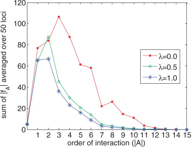
Sum of ’s averaged over 50 regions as a function of
Fig. 2.
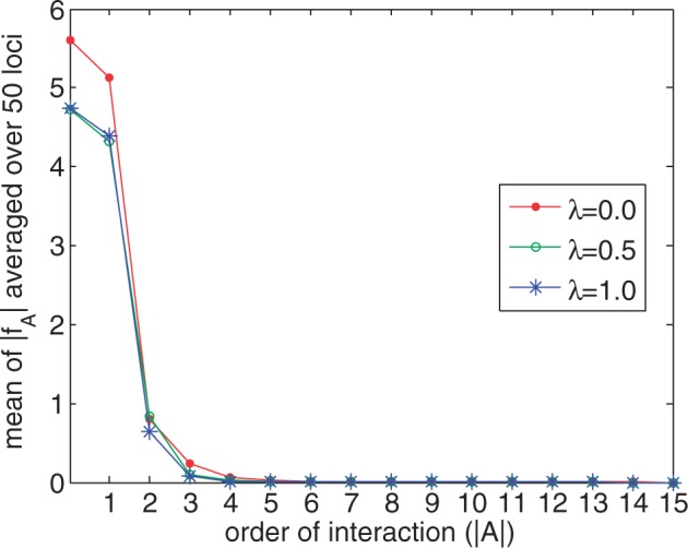
Mean of ’s averaged over 50 loci as a function of
Next we investigated how well the MVB fits the selected 1000 Genomes haplotypes using just lower-order interactions. To measure goodness of fit, we computed the Euclidean distance between the haplotype frequencies recovered by the MVB model as given in Equation (1) and the haplotype frequencies observed in the data. Table 1 demonstrates that the MVB model requires only the lower-order interactions terms to accurately fit typical data. Because attains the best fit across interaction level bounds (, we set λ to 0.25 in all future experiments.
Table 1.
Euclidean distance between haplotype frequencies recovered by the MVB model and haplotype frequencies observed in data for different values of max and λ
| Max | No. param. |
λ |
||||
|---|---|---|---|---|---|---|
| 0.0 | 0.25 | 0.5 | 0.75 | 1.0 | ||
| 1 | 16 | 0.348 | 0.348 | 0.348 | 0.348 | 0.348 |
| 2 | 121 | 0.137 | 0.072 | 0.073 | 0.074 | 0.075 |
| 3 | 576 | 0.120 | 0.054 | 0.055 | 0.056 | 0.056 |
| 4 | 1941 | 0.120 | 0.055 | 0.056 | 0.057 | 0.058 |
Bold values indicates the column attaining the best fit for the MVB model.
We also recorded the number of iterations until convergence of the coordinate descent algorithm. The algorithm invariably converges within 20–30 iterations. See Figure 3 for typical results. Finally, Table 2 lists that the bulk of computational time is taken in estimating MVB parameters; once model parameters are estimated, applying the model to making predictions is relatively trivial.
Fig. 3.
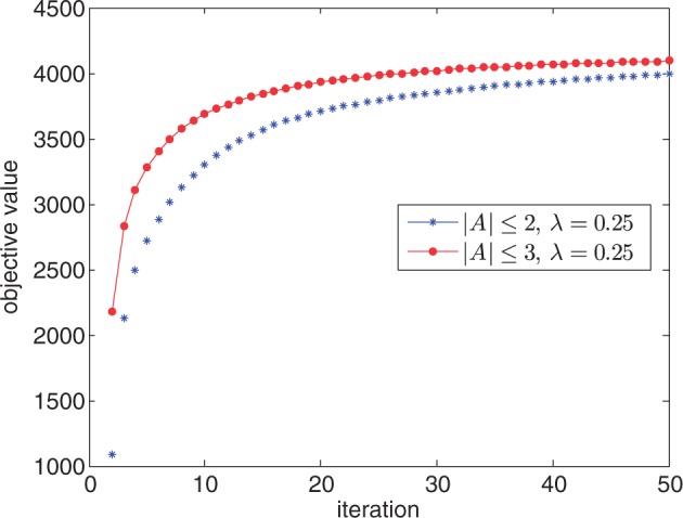
Objective value averaged over 50 loci at each iteration of the coordinate ascent algorithm for different values of max
Table 2.
Learning time (second per iteration) and prediction time (second per prediction), averaged over 50 loci
| Max | Learning (sec/iter) | Prediction (sec/pred) |
|---|---|---|
| 1 | 0.2 | <0.01 |
| 2 | 1.1 | <0.01 |
| 3 | 4.4 | 0.01 |
| 4 | 13.7 | 0.02 |
3.2 Prediction of DH status in simulations
To simulate binary DH data, we took the 1010 EUR (European) haplotypes of the 1000 Genome project (1000 Genomes Project Consortium et al., 2010) and simulated 20 000 haploid individuals at 200 randomly selected 20 kb regions on chromosome 1 (Su et al., 2011). From each region, we selected 15 SNPs with minor allele frequency above 1%. From the 15 chosen SNPs, we randomly selected m causal SNPs and n pairs of interaction SNPs and simulated continuous DH values according to the linear model sketched in Section 2.4. Prior to simulation, we standardized the SNP predictors hij and to have mean 0 and variance 1. The regression coefficients for the causal SNPs and SNP pairs were sampled as and and the noise for each DH variable as , where h2 and denote the variance of DH values explained by single variants and interactions, respectively. Finally, we converted the continuous DH values to binary DH values by imposing a threshold chosen so that 20% of the binary DH values were elevated (status 1 rather than status 0).
For testing under the MVB model, we constructed binary vectors of length 16 by concatenating each 15-SNP haplotype and a corresponding simulated binary DH status. Given the tuning constant , this allows us to estimate the fA parameters. To predict DH status given observed SNP haplotypes, one simply computes a conditional probability under the MVB model. In one set of MVB trials, we limited the interaction level to , for a total of 137 parameters. In a second set of trials, we limited the interaction level , for a total of 697 parameters. One can compare MVB prediction to BLUP and LOGIT prediction based on the same SNP haplotypes and interaction model. For BLUP and LOGIT, we also tested a model involving SNPs and interactions between adjacent SNPs.
In linear regression, Equation (10) supplies effect sizes, and Equation (11) supplies predicted values. In logistic regression, Equation (14) supplies predicted values. For estimation and prediction under HMM, we concatenated DH status as a pseudo SNP at the end of each 15-SNP haplotype to avoid changing the SNP interactions in the original haplotype. We also set the physical distance between the pseudo SNP and the last SNP to be the average distance between consecutive pairs of SNPs in the original 15-SNP haplotype. We employed half of the simulated individuals as reference panel and ran HMM with IMPUTE2 default settings on the other half to obtain predicted DH status. All 200 simulations summarized below involve two causal SNPs (m = 2) and two causal SNP interactions (n = 2) for 200 randomly sampled individuals. Of these 200 people, 100 served as training individuals and 100 as validation individuals.
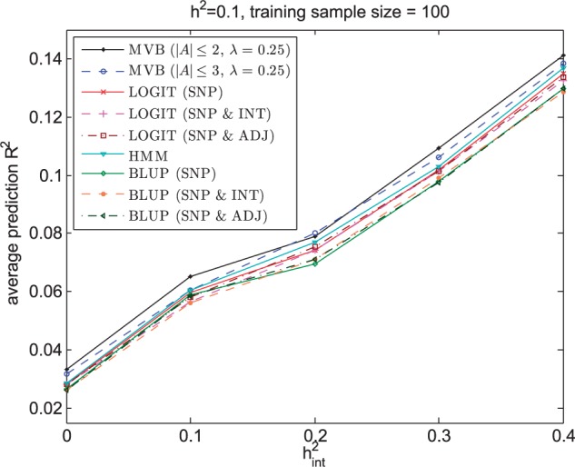
We first investigated performance of MVB, BLUP, LOGIT and HMM prediction for varying h2 for a fixed interaction of 0.1. Figure 4 shows that prediction R2 achieved by all models increases as h2 increases. However, the MVB model consistently achieves higher prediction R2 than BLUP, LOGIT and HMM under both settings, suggesting that the MVB model is capable of yielding more accurate estimates of effect sizes for prediction. Notably as h2 increases, the improvement in prediction R2 also increases. In other words, as the effect of a single SNP increases, the comparative advantage of the MVB model over BLUP, LOGIT and HMM increases.
Fig. 4.
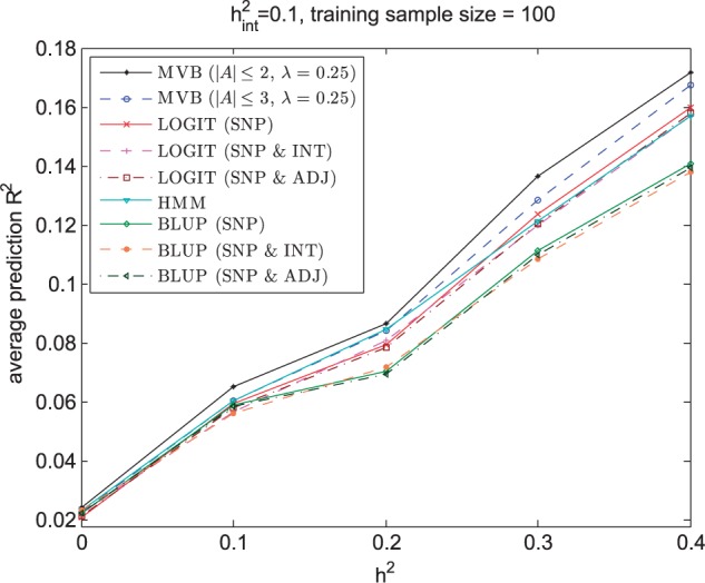
Prediction R2 across 100 validation individuals averaged over 200 regions for MVB, BLUP, LOGIT and HMM as a function of h2 when is fixed at 0.1
Next we investigated the accuracy of these approaches at varying values. Figure 5 demonstrates that for all pairs of h2 and , the MVB model also achieves higher prediction R2 than BLUP, LOGIT and HMM.
Fig. 5.
Prediction R2 across 100 validation individuals averaged over 200 regions for MVB, BLUP, LOGIT and HMM as a function of when h2 is fixed at 0.1
Finally, we investigated the number of samples required for accurate prediction. Figure 6 shows that although the MVB model requires more parameters than BLUP, LOGIT and HMM, it is able to outperform these models even if the training sample size is small. This suggests that the MVB model is less sensitive to noise. Notably, HMM under-performs both MVB and LOGIT in most simulation settings, suggesting that HMM is less capable of detecting long range interactions for reasonable sample sizes. Across all simulated datasets, we observe no major difference in prediction R2 between the two MVB settings. This is to be expected since only pairwise interactions are simulated.
Fig. 6.
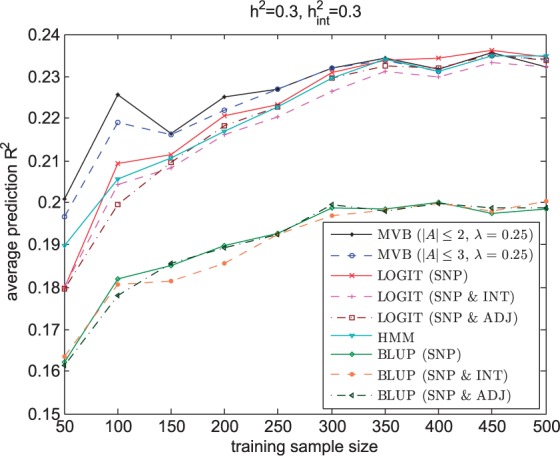
Prediction R2 across validation individuals averaged over 200 regions for the MVB, BLUP, LOGIT and HMM as a function of training sample sizes when h2 and are both fixed at 0.3
3.3 Predicting DH status in empirical data
We now turn to real data on DH status and reach similar conclusions. The dataset in question (Degner et al., 2012) contains normalized DH scores for 70 YRI (Yorubas in Ibadan, Nigeria) individuals at 1.5 million 100-bp genomic windows. These windows cover the 5% of the human genome with the highest DNaseI sensitivity. About half of the windows are expected to be truly sensitive to DNaseI (Boyle et al., 2008); 8902 windows have associated dsQTLs [SNPs showing significant correlations with DH scores across individuals (Degner et al., 2012)]. We dichotomized DH scores by placing scores above the threshold of 0.0 in one category and scores below the threshold of 0.0 in the complementary category. Among the 70 YRI individuals in the sample, 59 are also in the 1000 Genome project (1000 Genomes Project Consortium et al., 2010) and have fully phased haplotypes. We accordingly used the haplotypes and the binary DH status of these 59 individuals to evaluate the MVB model. For computational reasons, we selected one haplotype for each individual and restricted our analysis to 250 random DH sites and the 377 DH sites with associated dsQTLs on chromosome 22.
In genomic windows with associated dsQTLs, the dsQTLs are on average about 8000 base pairs (10 SNPs) away from their windows. This action at a distance renders it difficult for HMMs to accurately capture interactions between dsQTLs and their genomic windows. Because sequence order is an important factor for HMMs, the question also arises of where to place binary DH status (a pseudo SNP) in the haplotype. For this reason, we excluded HMM from comparisons on real data.
To avoid over-fitting, we assessed prediction accuracy by leave-one-out cross-validation. Thus, we estimated parameters using data from 58 (all but one) training individuals and predicted DH status for the remaining validation individual. Repeating this process across all 59 individuals allowed us to compare predicted and true DH status. The results can be summarized in a squared Pearson correlation (prediction R2). Prior to parameter estimation in each of the 59 folds, we selected a small number of relevant SNP predictors by linear regression and forward selection. Our selection procedure excluded SNPs with minor allele frequency below 1% or at a distance of 1 Mb or greater from the center of the window. Each successive SNP entering the candidate list provided the greatest reduction of the current residual sum of squares.
Given a candidate set of SNP predictors P in the MVB model, we created binary haplotype vectors of length from the SNPs and the binary DH status. We considered at most second-order interactions and set the penalty constant λ to 0.25. For BLUP and LOGIT, we considered three models, one limited to single SNPs, one involving both single SNPs and two-way interactions and one involving single SNPs and only interactions between adjacent SNPs.
Figure 7a shows the prediction R2 obtained through leave-one-out cross-validation averaged over the 250 randomly selected windows. Because of overfitting and our small sample size, the average prediction R2 decreases for all methods as the number of predictors increases. The MVB model achieves higher prediction R2 than BLUP and LOGIT over both settings. We repeated the same experiment on the 377 windows with associated dsQTLs. Again the MVB model consistently achieves higher prediction R2 than BLUP and LOGIT (Fig. 7b). Figure 7c and d depict the distribution of prediction R2’s under each model. It is clear that the MVB models achieve more high prediction R2’s (greater than 0.2) than BLUP and LOGIT. One can legitimately conclude that the MVB model predicts DH status better than BLUP and LOGIT. Table 3 summarizes the average and standard error of prediction R2 for some representative experiments.
Fig. 7.

Prediction R2 for MVB, BLUP and LOGIT. Here ‘SNP’ refers to the experiment involving only single SNPs, ‘SNP & INT’ refers to the experiment involving both SNPs and all two-way interactions and ‘SNP & ADJ’ refers to the experiment involving both SNPs and only interactions between adjacent SNPs. (a and b) The average prediction R2 over different windows as a function of the number of true predictors . (c and d) The distribution of prediction R2 for the highest average prediction R2 overall . For , the experiments ‘SNP & INT’ and ‘SNP & ADJ’ are identical
Table 3.
Average prediction R2 and standard error for over 250 randomly selected windows (RANDOM) and 377 windows with dsQTLs (dsQTL)
| MVB() | LOGIT | BLUP | ||
|---|---|---|---|---|
| RANDOM | 1 | 0.112 ± 0.015 | 0.093 ± 0.013 | 0.097 ± 0.013 |
| 2 | 0.109 ± 0.015 | 0.106 ± 0.015 | 0.100 ± 0.014 | |
| dsQTL | 1 | 0.120 ± 0.015 | 0.108 ± 0.015 | 0.114 ± 0.015 |
| 2 | 0.102 ± 0.014 | 0.100 ± 0.015 | 0.096 ± 0.014 |
4 Discussion
This article presents the MVB distribution as a vehicle for modeling haplotype data. Because the number of distinct haplotypes observed in a narrow genomic region tends to be small, the MVB model is typically wildly over-parameterized. To achieve parsimony, we propose a lasso penalty within a Poisson sampling framework. The penalized MVB model encourages the detection and exploitation of higher-order interactions among the underlying SNPs. In contrast to Markovian models, interactions extend beyond nearest neighbor and pairwise interactions. The interaction parameterization adopted here is more natural than the naive MVB parameterization implicitly seen in BLUP and LOGIT. Empirically, the interaction parameterization extracts more haplotype information and predicts with better accuracy.
Our application of the MVB model to predict DH status from observed haplotypes supports the utility of the model. We show that the MVB model achieves better accuracy than BLUP and LOGIT in predicting simulated DH status. The overall prediction R2 achieved by MVB, BLUP and LOGIT on real DH status suggests substantial heritability of this epigenetic signal.
In likelihood evaluation and parameter estimation, the computational complexity of the MVB models scales like for N SNPs. This harsh reality limits the applicability of the model to a small number of variants. Fortunately, even for small N, the MVB model offers valuable insights into genomic data. The MVB model may well be critical in predicting binary gene expression when a small number of causal variants localize within a gene. In particular, MVB profiles in cases and controls may help in fine mapping traits in genome-wide association studies. Overcoming the computational limits of the MVB model limit is high on our research agenda. Once this task is accomplished, it will be possible to apply the MVB model to pre-phasing, a technique for improving genotype imputation by first imputing haplotypes (Howie et al., 2012). We conjecture that Monte Carlo methods will play a decisive role in extending the range of the model to larger N. Finding an efficient sampling scheme to approximate the normalization constant is of paramount importance and doubtless the place to start in accelerating algorithm performance.
Acknowledgements
We thank Nicholas Mancuso and Gleb Kichaev for helpful discussions that improved the quality of our manuscript. We also thank the reviewers for their helpful comments and suggestions.
Funding
This research was supported by NIH (United States Public Health Service) grants GM53275 and HG006139.
Conflict of Interest: none declared.
References
- 1000 Genomes Project Consortium et al. (2010) A map of human genome variation from population-scale sequencing. Nature, 467, 1061–1073. [DOI] [PMC free article] [PubMed] [Google Scholar]
- Boyle A.P., et al. (2008) High-resolution mapping and characterization of open chromatin across the genome. Cell, 132, 311–322. [DOI] [PMC free article] [PubMed] [Google Scholar]
- Browning B.L., Browning S.R. (2011) A fast, powerful method for detecting identity by descent. Am. J. Hum. Genet., 88, 173–182. [DOI] [PMC free article] [PubMed] [Google Scholar]
- Browning S.R., Browning B.L. (2007) Rapid and accurate haplotype phasing and missing-data inference for whole-genome association studies by use of localized haplotype clustering. Am. J. Hum. Genet., 81, 1084–1097. [DOI] [PMC free article] [PubMed] [Google Scholar]
- Chung C.C., et al. (2013) Meta-analysis identifies four new loci associated with testicular germ cell tumor. Nat. Genet., 45, 680–685. [DOI] [PMC free article] [PubMed] [Google Scholar]
- Dai B., et al. (2013) Multivariate Bernoulli distribution. Bernoulli, 19, 1465–1483. [Google Scholar]
- Daly M.J., et al. (2001) High-resolution haplotype structure in the human genome. Nat. Genet., 29, 229–232. [DOI] [PubMed] [Google Scholar]
- de los Campos G., et al. (2013) Prediction of complex human traits using the genomic best linear unbiased predictor. PLoS Genet., 9, e1003608. [DOI] [PMC free article] [PubMed] [Google Scholar]
- Degner J.F., et al. (2012) DNase I sensitivity QTLs are a major determinant of human expression variation. Nature, 482, 390–394. [DOI] [PMC free article] [PubMed] [Google Scholar]
- Gibbs R.A., et al. (2003) The international hapmap project. Nature, 426, 789–796. [DOI] [PubMed] [Google Scholar]
- Howie B.N., et al. (2009) A flexible and accurate genotype imputation method for the next generation of genome-wide association studies. PLoS Genet., 5, e1000529. [DOI] [PMC free article] [PubMed] [Google Scholar]
- Howie B., et al. (2012) Fast and accurate genotype imputation in genome-wide association studies through pre-phasing. Nat. Genet., 44, 955–959. [DOI] [PMC free article] [PubMed] [Google Scholar]
- Kruglyak L. (1999) Prospects for whole-genome linkage disequilibrium mapping of common disease genes. Nat. Genet., 22, 139–144. [DOI] [PubMed] [Google Scholar]
- Lange K. (2010) Applied Probability. Springer Texts in Statistics. Springer, New York. [Google Scholar]
- Lange K. (2013) Optimization. Springer Texts in Statistics. Springer, New York. [Google Scholar]
- Lawson D.J., et al. (2012) Inference of population structure using dense haplotype data. PLoS Genet., 8, e1002453. [DOI] [PMC free article] [PubMed] [Google Scholar]
- Li N., Stephens M. (2003) Modeling linkage disequilibrium and identifying recombination hotspots using single-nucleotide polymorphism data. Genetics, 165, 2213–2233. [DOI] [PMC free article] [PubMed] [Google Scholar]
- Li Y., et al. (2010) Mach: using sequence and genotype data to estimate haplotypes and unobserved genotypes. Genet. Epidemiol., 34, 816–834. [DOI] [PMC free article] [PubMed] [Google Scholar]
- Lohmueller K.E., et al. (2009) Methods for human demographic inference using haplotype patterns from genomewide single-nucleotide polymorphism data. Genetics, 182, 217–231. [DOI] [PMC free article] [PubMed] [Google Scholar]
- Madrigal P., Krajewski P. (2012) Current bioinformatic approaches to identify DNase I hypersensitive sites and genomic footprints from DNase-seq data. Front. Genet., 3. [DOI] [PMC free article] [PubMed] [Google Scholar]
- Marchini J., et al. (2007) A new multipoint method for genome-wide association studies by imputation of genotypes. Nat. Genet., 39, 906–913. [DOI] [PubMed] [Google Scholar]
- Morris A.P. (2006) A flexible Bayesian framework for modeling haplotype association with disease, allowing for dominance effects of the underlying causative variants. Am. J. Hum. Genet., 79, 679–694. [DOI] [PMC free article] [PubMed] [Google Scholar]
- Pasaniuc B., et al. (2009) Inference of locus-specific ancestry in closely related populations. Bioinformatics, 25, i213–i221. [DOI] [PMC free article] [PubMed] [Google Scholar]
- Pool J.E., et al. (2010) Population genetic inference from genomic sequence variation. Genome Res., 20, 291–300. [DOI] [PMC free article] [PubMed] [Google Scholar]
- Price A.L., et al. (2008) Long-range ld can confound genome scans in admixed populations. Am. J. Hum. Genet., 83, 132. [DOI] [PMC free article] [PubMed] [Google Scholar]
- Price A.L., et al. (2009) Sensitive detection of chromosomal segments of distinct ancestry in admixed populations. PLoS Genet., 5, e1000519. [DOI] [PMC free article] [PubMed] [Google Scholar]
- Savage S.A., et al. (2013) Genome-wide association study identifies two susceptibility loci for osteosarcoma. Nat. Genet., 45, 799–803. [DOI] [PMC free article] [PubMed] [Google Scholar]
- Scheet P., Stephens M. (2006) A fast and flexible statistical model for large-scale population genotype data: applications to inferring missing genotypes and haplotypic phase. Am. J. Hum. Genet., 78, 629–644. [DOI] [PMC free article] [PubMed] [Google Scholar]
- Su Z., et al. (2011) Hapgen2: simulation of multiple disease SNPs. Bioinformatics, 27, 2304–2305. [DOI] [PMC free article] [PubMed] [Google Scholar]
- Templeton A.R. (2005) Haplotype trees and modern human origins. Am. J. Phys. Anthropol., 128, 33–59. [DOI] [PubMed] [Google Scholar]
- Wall J.D., Pritchard J.K. (2003) Haplotype blocks and linkage disequilibrium in the human genome. Nat. Rev. Genet., 4, 587–597. [DOI] [PubMed] [Google Scholar]
- Yang W.-Y., et al. (2014) A spatial-aware haplotype copying model with applications to genotype imputation. In: Sharan R. (ed.), Research in Computational Molecular Biology. Springer International Publishing, Switzerland, pp. 371–384. [Google Scholar]