

Abstract
Inadequate statistical power to detect treatment effects in health research is a problem that is compounded when testing for mediation. In general, the preferred strategy for increasing power is to increase the sample size, but there are many situations where additional participants cannot be recruited, necessitating the use of other methods to increase statistical power. Many of these other strategies, commonly applied to analysis of variance and multiple regression models, can be applied to mediation models with similar results. Additional predictors or blocking variables will increase or decrease statistical power, however, depending on whether these variables are related to the mediator, the outcome, or both. The effect of these two methods on the power for tests of mediation is illustrated through the use of simulations. Implications for health researchers using these methods are discussed.
Keywords: mediation, statistical power, sample size
Due to the work of Cohen (1988) and others (e.g., Freiman, Chalmers, Smith, & Kuebler, 1978), most health researchers recognize the need for adequate statistical power. In addition to an increased ability to detect effects, adequate statistical power is a requirement when applying for grants. As noted by Murray (2008), “[U]nless the reviewers are satisfied that the investigators have . . . shown that the power is adequate, their enthusiasm will be reduced, with a consequent reduction in the likelihood that the project will receive a good priority score” (p. 89). Health researchers have also become more focused on understanding mechanisms of change when evaluating randomized controlled trials (RCTs) and prevention interventions. The primary method for examining mechanisms of change statistically is mediation analysis, where the intervention or treatment affects the outcome variable through a third intervening variable.
A variety of statistical tests have been developed to test whether a variable mediates a specific effect, each with a different level of statistical power depending on the situation (e.g., MacKinnon, Lockwood, Hoffman, West, & Sheets, 2002; MacKinnon, Lockwood, & Williams, 2004). Fritz and MacKinnon (2007) selected six tests of mediation, based on popularity and statistical power, and estimated the required sample size necessary to achieve power of .80 for combinations of small, medium, and large effects to help researchers adequately power their mediation studies. The most common question raised by readers of the Fritz and MacKinnon study is: Can anything be done to increase power in tests of mediation when the desired sample size cannot be obtained? Sample size is of special concern to health professionals when the prevalence of a disease or disorder is low, recruitment of participants is difficult, or the costs of collecting additional data are prohibitive. Fortunately, there are numerous ways to increase power for statistical tests without increasing sample size (McClelland, 2000). Certain methods, however, such as including additional predictors and blocking may be less straightforward for mediation models because the gain in power is dependent on whether the additional predictor or blocking variable is related to the mediator, the outcome variable, or both. The current project examines how these two methods can increase the power of tests of mediation.
The Single Mediator Model
The single mediator model refers to a special case of the more general class of third variable models where change in an independent variable X causes change in an outcome variable Y through a third intervening or mediating variable M. Mediation is distinct from other third variable models such as confounding, where the third variable causes both X and Y, or moderation, where the magnitude and sign of the effect of X on Y are dependent on the value of the third variable. The single mediator model, illustrated in Figure 1, can be estimated using three regression equations
Figure 1.
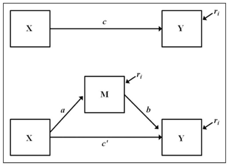
The single mediator model.
| (1) |
| (2) |
| (3) |
where c1 is the total effect of X on Y, a1 is the effect of X on M, b1 is the effect of M on Y controlling for X, c′1 is the direct effect of X on Y controlling for M, β0 is an intercept, and ri are residuals. The a effect is referred to as the action theory in RCT and intervention research because participants are actively assigned to levels of the treatment variable X (Chen, 1990). The b effect is referred to as the conceptual theory because participants are rarely assigned to levels of the mediator so the link between the mediator and the outcome must instead rely on the conceptual theory (MacKinnon, Taborga, & Morgan-Lopez, 2002). The mediated or indirect effect is equal to ab, provided certain assumptions are met including no confounding of the X to M, X to Y, or M to Y relations, especially by other variables affected by the treatment (VanderWeele & Vansteelandt, 2009).
Statistical Power for Mediation Models
The power of a statistical test is the probability of rejecting the null hypothesis when the null hypothesis is false. That is, power is the probability of finding an effect when an effect is present. Statistical power is dependent on three values: the Type I error rate, the sample size, and the effect size. In general, as any of these quantities increases while the other two remain constant, power increases. In most a priori power analyses, the desired power, Type I error rate, and expected effect size are selected, so that the required sample size can be computed. In a sensitivity analysis, the effect size that can be detected for a specific Type I error rate, sample size, and power level is calculated. A power level of .80 is commonly used by behavioral scientists (Cohen, 1988), but health researchers may require higher power or accept lower power depending on the type of research they are conducting. Researchers are most concerned with studies that are under-powered, but researchers must also be concerned with studies that are overpowered, usually due to extremely large sample sizes. In an overpowered study, effects may be statistically significant but have little or no practical significance. Multiple methods for dealing with overpowered studies exist, including using a more conservative Type I error level or setting a minimum effect size below which a statistically significant effect will not be interpreted.
Calculating the required sample size for a specific power level in mediation models is more complex than for many other statistical tests because the power to detect both a and b must be taken into account. This is why most power analysis programs do not directly compute power for mediation models and the reason a majority of the prior work on power in mediation has been conducted using simulations (e.g., Hoyle & Kenny, 1999; MacKinnon, Lockwood, et al., 2002). A general method to determine power in a variety of different mediational designs, including structural equation models, models with multiple mediators, and mediation with missing and nonnormal data, was developed by Thoemmes, MacKinnon, and Reiser (2010). Using the “Monte Carlo” command in Mplus (Muthen & Muthen, 2013), the authors created syntax that can estimate the power for the mediated effect by entering expected values for a and b. These power estimates are calculated using the first-order standard error test (Sobel, 1982), which may underestimate power for other tests of mediation, though these estimates can then be entered into PRODuct Confidence Limits for INdirect effects (PRODCLIN; MacKinnon, Fritz, Williams, & Lockwood, 2007) to determine power for the distribution of the product test (MacKinnon et al., 2002; Meeker, Cornwell, & Aroian, 1981).
In order to discuss methods for increasing power in mediation models without increasing the sample size, clarification is needed for how increasing sample size actually increases power. Increasing the sample size decreases the standard error of the mediated effect, which in turn increases the power. Consider the first-order standard error for the standardized mediated effect (Sobel, 1982) where the asterisks indicate standardized coefficients
| (4) |
In the standard error, is the squared correlation between X and M, and is equal to the squared multiple correlation of Y regressed on X and M. Equation 4 shows that when all other quantities are held constant, the standard error decreases as the sample size n increases. Any change that decreases the standard error of a test of mediation will increase power, however, even if the sample size does not change.
Numerous methods exist for reducing the standard error of a statistic without increasing the sample size that can be applied to mediation models. Using modern missing data techniques including full-information maximum likelihood and multiple imputation (Enders, 2010; Schafer & Graham, 2002) or designs with planned missingness (Graham, Taylor, & Cumsille, 2001) will increase the number of cases that can be used to estimate the mediation model without increasing the initial sample size. The use of structural equation models to model measurement error in a mediation model has been shown to return smaller standard error estimates than multiple regression models (Hoyle & Kenny, 1999; Iacobucci, Saldanha, & Deng, 2007). Sampling variables across a larger range can decrease standard errors (McClelland, 2000), as can the use of repeated measures (Venter & Maxwell, 1999). Blocking and the inclusion of additional predictors can also decrease the standard error. Unlike the other methods just described, however, the amount the statistical power of a test of mediation increases for these two methods is more complicated because it depends on whether the additional predictors or the blocking variable are related to the mediator, the outcome, or both, as well as other factors.
Additional Predictors
The first method considered here to decrease the standard error of a test of mediation without increasing the sample size is to include additional predictors. Consider again the standard error formula in Equation 4 where is the residual variance in M not explained by X, and is the residual variance in Y not explained by X and M. Since these quantities appear in the numerator, as the percentage of explained variance in either M or Y increases, the standard error decreases. Hence, adding predictors to the model that explain additional variance in M or Y will increase power, but there are two penalties for adding additional predictors. The first penalty is the quantity (n – p – 1), which adjusts the standard error for the total number of predictors in the model p, so that as p increases while the variance explained remains constant, the standard error increases. The second penalty is the variance inflation factor (VIF), , which is a measure of the multicollinearity of X and M, and increases the standard error as the redundancy between predictors increases. In order to decrease the standard error by including additional predictors, the gain in explained variance in M or Y must be larger than the penalty for increasing p or the VIF.
The interplay between variance explained, number of predictors, and the VIF leads to the counterintuitive situation where the power of the test of b increases as the size of c′ increases if b stays constant. That is, there is more power to test for a mediator that explains a smaller proportion of the total effect. To understand why, consider that in Equation 4 the standard error of b will increase as X explains less of the variance in Y. This means the standard error for b will be largest when c′ = 0 because will be at its smallest. The situation is compounded when a is large, because the VIF will also increase. This means that as the size of a increases, the power to detect b can decrease, especially when b is a small effect (Fritz, Taylor, & MacKinnon, 2012; Hoyle & Kenny, 1999; MacKinnon, 2008). Hansen and McNeal (1996, p. 502) call this phenomenon “the law of maximum expected potential effect, which specifies that the magnitude of change in behavioral outcome that a program can produce is directly limited by the strength of the relations that exist between mediators and targeted behaviors.”
Based on these considerations, several categories of variables are good candidates for inclusion as additional predictors in a mediation model. The first are prior measurements of M and Y such as pretest measures (Venter & Maxwell, 1999), including baseline measures taken before implementation of an RCT. These autoregressive effects are often quite large and excluding them is equivalent to constraining these effects to zero (Gollob & Reichardt, 1987), which will bias the estimates of the mediation parameters when untrue (Maxwell & Cole, 2007). Steyer, Fiege, and Rose (2010) go a step further and state that whenever possible, pretest measures of M and Y should be included in the model. A second category of predictors are demographic variables such as age and gender, which are often controlled for in RCTs. A third category is the inclusion of interaction terms, although interactions that include mediators are beyond the scope of this article (see, e.g., Fairchild & MacKinnon, 2009). A fourth, and perhaps the most important, category of variables are other potential mediators of the relation between the treatment and the outcome. Additional mediators can increase power while also producing a more accurate estimate of the original mediator by controlling for the shared effects of the additional mediators. Hansen and McNeal (1996) argue that in behavioral interventions any direct effect between X and Y is most likely due to the exclusion of additional mediating variables from the model.
Blocking
When individuals are randomly assigned to levels of treatment, the power to detect the mediated effect can also be increased through the use of blocking variables. In a completely randomized (CR) design, individuals are assigned to treatments at random, ignoring all personal characteristics. A completely blocked (CB) design involves selecting a variable that explains variance in the outcome variable, randomizing individuals within levels of the blocking variable to the levels of the treatment, and then including the blocking variable in the model. For example, if gender is related to the outcome variable, instead of randomly assigning all individuals to treatments, a researcher would randomize females and males to treatments separately so there would be an equal ratio of males and females in each of the treatment levels. Blocking variables can be socioeconomic variables such as education level or risk variables such as condom use, but can also be any other variable related to the outcome.
Compared to a CR design, blocking reduces the experimental error (i.e., residual variance) by creating homogeneous groups of individuals so that the variance within each block is smaller than the variance of individuals across blocks (Kuehl, 2000). For mediation models, this means the blocking variable explains variance in M or Y so that the residual variances or in Equation 4 are smaller for a CB design than for a CR design, resulting in an increase in power. As with the inclusion of additional predictors, however, there are some caveats to this increase in power. The first issue, as described by Kuehl, is that as the number of levels of the blocking variable increases, the degrees of freedom for the blocking variable also increases, which increases p. As p increases, the quantity (n – p – 1) in Equation 4 decreases, increasing the standard error and decreasing power.
The second issue involves whether the blocking variable is related to M, Y, or both. In a mediation model where individuals are randomly assigned to levels of X using a CB design, the blocking variable and X will be uncorrelated when each level of X has an equal ratio of individuals in the levels of the blocking variable. If the blocking variable is related to both M and Y, the power for a will increase as decreases, but the effect on the power for b depends on the correlation between the blocking variable and M, and the amount that decreases. If the VIF increases less than the residual variance decreases, then the power will increase; otherwise it will decrease. This means the overall power for the mediated effect may increase, stay the same, or even decrease slightly. The same issues with the relations between X, M, and the blocking variable must be considered when the blocking variable is only related to Y. When the blocking variable is related only to M and is uncorrelated with X, the power to detect a will increase as decreases, but the power for b should remain the same.
Simulations
The exact amount blocking or adding an additional predictor to a mediation model will increase statistical power is difficult to determine because it is dependent on many factors. For example, the size of a, b, and the effect of the additional predictor, whether the additional predictor is related to M, Y, or both, and the original power to detect the mediated effect. In order to illustrate specifically how blocking and including additional predictors affects the power to detect mediation for specific parameter conditions, a series of simulations were conducted. All simulations were conducted using R (R Core Development Team, 2012). Six different tests of mediation were used in each simulation: the Baron and Kenny (1986) causal steps test, the joint significance test (MacKinnon et al., 2002), Sobel’s (1982) first-order standard error test, the PRODCLIN distribution of the product test (MacKinnon et al., 2007), the percentile bootstrap test, and the bias-corrected bootstrap test (Bollen & Stein, 1990; Efron & Tibshirani, 1993; Shrout & Bolger, 2002). For more information on these tests, see MacKinnon (2008).
Simulation #1
The first simulation investigated the impact of adding additional predictors to the single mediator model that are uncorrelated with the predictors already in the model. Two new variables were introduced: W is an additional predictor that explains variance in M, but is uncorrelated with X; and V is an additional predictor that explains variance in Y, but is uncorrelated with X or M. Data for X, W, and V were generated from standard normal distributions using RNORM in R. M and Y were generated using Equations 1–3 and
| (5) |
| (6) |
where d represents the effect of W on M controlling for X and e represents the effect of V on Y controlling for M and X. The effect sizes for a, b, d, and e were varied between 0.14, 0.39, and 0.59, which correspond to small, medium, and large partial effects (Cohen, 1988). Because changing the values of c′ would distort the effects of the added predictors, c′ was set equal to 0 for all conditions to represent the worst-case scenario in terms of power where X explains no variance in Equation 3 or 6, increasing the standard error of b. All combinations of effect sizes for a and b were investigated (e.g., a–b: small–small, small–medium, etc.), while d and e were set equal (i.e., d–e: small–small, medium–medium, large–large) resulting in 27 combinations.
Sample size is important because overpowering the tests would cause ceiling effects that would obscure the change in power. For that reason, the sample sizes from Fritz and MacKinnon (2007) for the joint significance test, which has power greater than the Baron and Kenny causal steps test and less than the bias-corrected bootstrap test, were multiplied by 0.75 to emulate the situation where a researcher is unable to attain the sample size necessary for .80 power and are shown in Table 1. The six tests of mediation were then conducted on each combination of parameters from Equation 2, 3, 5, and 6 (i.e., a1b1, a1b2, a2b1, and a2b2). This process of generating data and testing for mediation was repeated 1,000 times and the proportion of replications where significant mediation was found for a specific test was equal to the statistical power for that test and for that effect size combination.
Table 1.
Change in Power When an Additional Predictor of M Is Included in the Model (i.e., a2b1 – a1b1).
| Test | d | ab = SS (n = 398) | SM (n = 302) | SL (n = 302) | MS (n = 304) | MM (n = 56) | ML (n = 44) | LS (n = 304) | LM (n = 44) | LL (n = 27) |
|---|---|---|---|---|---|---|---|---|---|---|
| Baron and Kenny | S | .000 | .001 | .000 | .000 | .000 | −.001 | .000 | .000 | −.005 |
| M | .003 | .001 | .009 | .000 | .005 | .004 | .000 | .001 | −.002 | |
| L | .006 | .011 | .008 | .000 | .005 | .010 | .000 | .005 | .010 | |
| Joint | S | .000 | −.001 | .000 | .000 | .005 | −.003 | .000 | .001 | −.005 |
| M | .044 | .061 | .053 | .000 | .047 | .045 | .000 | .018 | .027 | |
| L | .060 | .122 | .123 | .000 | .089 | .094 | .000 | .049 | .090 | |
| Sobel | S | −.001 | .008 | .000 | .000 | .000 | −.004 | .000 | −.009 | −.005 |
| M | .065 | .070 | .055 | .005 | .050 | .058 | .001 | .028 | .043 | |
| L | .080 | .121 | .121 | .018 | .121 | .099 | .007 | .062 | .090 | |
| Distribution of the Product (PRODCLIN) | S | .004 | −.002 | −.002 | .000 | −.003 | −.003 | .000 | .005 | −.001 |
| M | .046 | .058 | .054 | −.004 | .051 | .048 | −.001 | .016 | .030 | |
| L | .060 | .123 | .121 | −.005 | .090 | .102 | .000 | .049 | .068 | |
| Percentile | S | .014 | .006 | .004 | .000 | −.002 | .002 | .000 | −.003 | −.018 |
| M | .049 | .065 | .070 | .000 | .044 | .068 | .000 | .019 | .020 | |
| L | .056 | .124 | .123 | .000 | .077 | .099 | .000 | .062 | .065 | |
| Bias corrected | S | .002 | −.002 | .000 | −.002 | −.005 | −.020 | .000 | −.019 | −.011 |
| M | .052 | .058 | .064 | .002 | .031 | .055 | −.004 | .011 | .004 | |
| L | .050 | .134 | .121 | −.005 | .095 | .089 | .000 | .058 | .055 |
Note. PRODCLIN = PRODuct Confidence Limits for INdirect effects.
S (small) = .14, M (medium) = .39, L (large) = .59, a1 is the effect of X on M, a2 is the effect of X on M controlling for the additional predictor W, b1 is the effect of M on Y controlling for X, and d is the effect of the additional predictor W on M controlling for X. Positive values reflect an increase in statistical power when the additional predictor W is added to the model.
The difference in power when an additional predictor of M is included in the estimation of a (i.e., Equation 5 is used in place of Equation 2) is illustrated in Table 1. As can be seen from the table, including an additional predictor of the mediator can increase the power of a test. For example, when a is a small effect, b is a large effect, and the effect of the additional predictor is medium, the power increased by .053 for the joint significance test, .054 for the distribution of the product test, .055 for the first-order standard error test, .064 for the bias-corrected bootstrap test, and .070 for the percentile bootstrap test. For the same values of a and b, when the effect of the additional predictor is large, the first-order, distribution of the product, and bias-corrected bootstrap tests increased by .121, while the joint significance and percentile bootstrap tests increased by .123. The increase in power, however, is contingent on the model having enough power to detect the effect of the additional predictor. If the study is underpowered to detect the extra predictor, no additional variance in the dependent variable is accounted for and the added predictor may increase the standard error. This is illustrated by the negative values in the table such as the value −.002 for the distribution of the product test when a is small, b is large, and the effect of the additional predictor is small. In addition, because W affects the standard error of a but not b, conditions where b is the smaller, limiting effect did not see a gain in power. For example, when a is large and b is small, the difference in power for all tests is approximately zero. Note that PRODCLIN did not converge for a small percentage of iterations (.005 or less for a particular set of mediation parameters), which is due to numerical integration issues that can occur when one of the confidence limits approaches zero. There is no evidence that nonconvergence is based on the significance of the mediated effect, so the power for PRODCLIN was computed for the number of replications that converged for this and all other simulations presented here.
Table 2 shows the difference in power when an additional predictor of Y is included in the model (i.e., Equation 6 is used in place of Equation 3). The magnitude of the changes in power are similar to Table 1, but V affects the standard error of b and not a, so conditions where a is the smaller, limiting effect now have no gain in power. For example, in Table 1 the condition where a is a large effect, b is a small effect, and the effect of the additional predictor is large showed almost no change in power. In Table 2, for the same values, the power increases from .030 for the Baron and Kenny causal steps test to .143 for the first-order standard error test, while the additional predictor has no effect on power when a is small and b is large, the opposite of Table 1.
Table 2.
Change in Power When an Additional Predictor of Y Is Included in the Model (i.e., a1b2 – a1b1).
| Test | e | ab = SS (n = 398) | SM (n = 302) | SL (n = 302) | MS (n = 304) | MM (n = 56) | ML (n = 44) | LS (n = 304) | LM (n = 44) | LL (n = 27) |
|---|---|---|---|---|---|---|---|---|---|---|
| Baron and Kenny | S | .000 | .000 | .000 | .001 | −.002 | −.001 | .000 | −.006 | −.007 |
| M | .002 | .000 | .000 | .004 | .004 | .004 | .005 | .005 | .020 | |
| L | .002 | .000 | .000 | .019 | .017 | .004 | .030 | .024 | .019 | |
| Joint | S | .010 | .000 | .000 | .015 | −.009 | .000 | .010 | −.010 | −.018 |
| M | .041 | .000 | .000 | .049 | .026 | .008 | .037 | .045 | .035 | |
| L | .061 | .000 | .000 | .118 | .068 | .016 | .138 | .097 | .053 | |
| Sobel | S | .005 | .000 | .002 | .001 | −.010 | −.009 | .011 | −.010 | −.012 |
| M | .045 | .005 | .001 | .046 | .041 | .040 | .030 | .035 | .055 | |
| L | .086 | .008 | .004 | .122 | .085 | .048 | .143 | .106 | .075 | |
| Distribution of the Product (PRODCLIN) | S | .008 | .000 | .000 | .013 | −.010 | −.005 | .006 | −.009 | −.007 |
| M | .042 | −.002 | .000 | .048 | .027 | .010 | .028 | .052 | .025 | |
| L | .061 | −.003 | −.001 | .117 | .076 | .014 | .139 | .090 | .048 | |
| Percentile | S | .018 | .000 | .000 | .008 | −.007 | −.007 | .001 | −.015 | −.010 |
| M | .045 | .000 | .000 | .043 | .014 | .016 | .047 | .045 | .026 | |
| L | .068 | .000 | .000 | .130 | .069 | .022 | .134 | .090 | .055 | |
| Bias corrected | S | .001 | −.001 | −.002 | .010 | −.021 | −.006 | .009 | −.021 | −.008 |
| M | .043 | .002 | −.007 | .051 | −.002 | .020 | .045 | .055 | .018 | |
| L | .057 | −.002 | −.003 | .113 | .080 | .006 | .136 | .075 | .049 |
Note. PRODCLIN = PRODuct Confidence Limits for INdirect effects.
S (small) = .14, M (medium) = .39, L (large) = .59, a1 is the effect of X on M, b1 is the effect of M on Y controlling for X, b2 is the effect of M on Y controlling for X and the additional predictor V, and e is the effect of the additional predictor V on Y controlling for M and X. Positive values reflect an increase in statistical power when the additional predictor V is added to the model.
Table 3 shows the change in power when additional predictors of M and Y are both included (i.e., Equations 5 and 6 were used instead of Equations 2 and 3). By including both W and V, the changes in power are larger and there are no combinations of a and b where power was unchanged. For example, when a and b are medium effects and the effect of the additional predictor is large, the increase in power for the distribution of the product test when there are additional predictors of both M and Y is .175, compared to .090 when there is only an additional predictor of M and .076 when there is only an additional predictor of Y.
Table 3.
Change in Power When Additional Predictors of M and Y Are Included in the Model (i.e., a2b2 – a1b1).
| Test | d, e | ab = SS (n = 398) | SM (n = 302) | SL (n = 302) | MS (n = 304) | MM (n = 56) | ML (n = 44) | LS (n = 304) | LM (n = 44) | LL (n = 27) |
|---|---|---|---|---|---|---|---|---|---|---|
| Baron and Kenny | S, S | .000 | .001 | .000 | .001 | −.002 | −.002 | .000 | −.006 | −.011 |
| M, M | .005 | .001 | .009 | .004 | .008 | .008 | .005 | .007 | .018 | |
| L, L | .009 | .011 | .008 | .019 | .022 | −.168 | .030 | .029 | .030 | |
| Joint | S, S | .011 | −.001 | .000 | .015 | −.004 | −.004 | .010 | −.009 | −.023 |
| M, M | .091 | .061 | .053 | .049 | .073 | .054 | .037 | .063 | .062 | |
| L, L | .133 | .122 | .123 | .118 | .170 | .115 | .138 | .158 | .152 | |
| Sobel | S, S | .012 | .007 | .000 | .001 | −.017 | −.009 | .012 | −.013 | −.013 |
| M, M | .107 | .073 | .055 | .055 | .090 | .095 | .031 | .071 | .091 | |
| L, L | .176 | .128 | .129 | .135 | .212 | .163 | .151 | .183 | .176 | |
| Distribution of the Product (PRODCLIN) | S, S | .016 | −.003 | −.002 | .013 | −.009 | −.006 | .006 | −.006 | −.008 |
| M, M | .091 | .057 | .054 | .047 | .076 | .053 | .028 | .063 | .059 | |
| L, L | .130 | .122 | .117 | .114 | .175 | .119 | .138 | .146 | .122 | |
| Percentile | S, S | .026 | .006 | .004 | .008 | −.012 | −.006 | .001 | −.018 | −.024 |
| M, M | .103 | .065 | .070 | .043 | .062 | .079 | .047 | .055 | .048 | |
| L, L | .145 | .124 | .123 | .130 | .158 | .118 | .134 | .154 | .130 | |
| Bias corrected | S, S | .006 | −.004 | .004 | .007 | −.015 | −.024 | .007 | −.031 | −.015 |
| M, M | .091 | .059 | .061 | .044 | .048 | .060 | .045 | .050 | .035 | |
| L, L | .124 | .128 | .118 | .111 | .157 | .094 | .131 | .126 | .095 |
Note. PRODCLIN = PRODuct Confidence Limits for INdirect effects.
S (small) = .14, M (medium) = .39, L (large) = .59, a1 is the effect of X on M, a2 is the effect of X on M controlling for the additional predictor W, b1 is the effect of M on Y controlling for X, b2 is the effect of M on Y controlling for X and the additional predictor V, d is the effect of the additional predictor W on M controlling for X, and e is the effect of the additional predictor V on Y controlling for M and X. Positive values reflect an increase in statistical power when the additional predictors W and V are added to the model.
The results show that including additional predictors can substantially increase power, but it may also decrease power. Consider the condition in Table 3 that lead to the largest increase in power for all of the tests where a and b are medium effects and d and e are large effects. The reason this condition resulted in the largest increase in power is that the additional predictors W and V were uncorrelated with X and M, so no additional variance was partialed out of a and b. At the same time, the sample size of 56 was large enough to reliably detect the large d and e effects. As described in Equation 4, this leads to an ideal situation where the additional predictors are reliably explaining extra variance in M and Y, while not increasing the VIF, which greatly decreases the standard error of the mediated effect and increased power. If we change any of these factors, the change in power decreases. For example, if d and e are medium effects while the sample size, a, and b remain the same, the power to reliably detect the effects of W and V decreases. This results in a smaller increase in power for the mediated effect because when d and e are not significant, they do not add as much to the variance explained, but they do add to the number of predictors in the model, so the standard error does not decrease. This is further illustrated when d and e are small effects and the power to detect the mediated effect was lower when W and V are included in the model than when they were not included.
Based on these results, including additional predictors in a mediation model is not a panacea for power issues. First, there must be adequate power to detect the effect of the additional predictors or the power to detect the mediated effect may decrease. Second, additional predictors only increase power if they affect the standard error of the smaller, limiting effect; otherwise, the power will remain unchanged. Third, as the number of new predictors increases, while the gain in explained variance remains the same, any increase in power will diminish as a function of the penalty paid for the total number of predictors in the model. Fourth, a large correlation between predictors will cause the VIF to increase, potentially diminishing any increase in power gained by including the additional predictor or even decreasing power. Finally, when the new predictors are correlated with X and/or M, the magnitude of a and/or b will likely also be diminished when the new predictor is partialed out, also decreasing power.
Simulation #2
The second simulation is identical to the previous simulation with the exception that a medium-sized effect (i.e., 0.39) was included between X and W, and between M and V to illustrate the case where the predictors are correlated. In Table 4, the negative values show the decrease in statistical power between the mediated effect from Equations 5 and 6, a2b2, from the first simulation when there is no correlation between the additional predictor and the mediation variables, and a2b2 from the second simulation when a medium-sized relation existed. As can be seen in the table, the statistical power was reduced in all situations. For example, when a is a large effect and b is a small effect, the power decreased from −.045 to −.100 compared to the same parameter values in Table 3. When the sample size is large enough to provide adequate power to detect the effect of the additional predictor, the effect of the nonzero relation between the additional predictor and the mediation variables was to reduce the original gain in power achieved through the inclusion of the additional predictors. When the sample size was not large enough to provide adequate power to detect the effects of the additional predictors, the power for finding the mediated effect decreased below the level of power found using the original mediation equations that did not include additional predictors (i.e., Equations 2 and 3). In addition, if a study is overpowered to begin with, including additional predictors will have little or no effect in terms of increasing power, but could decrease power. For example, when a, b, and the additional predictors were all medium effects, the increase in power for the bias-corrected bootstrap test when the predictors were uncorrelated is .048, but when the predictors are correlated the power decreases by .060, an overall decrease in power of .012.
Table 4.
Change in Power When Additional Predictors of M and Y Have a Medium Correlation With X and M (i.e., a2b2 – a2b2).
| Test | d, e | ab = SS (n = 398) | SM (n = 302) | SL (n = 302) | MS (n = 304) | MM (n = 56) | ML (n = 44) | LS (n = 304) | LM (n = 44) | LL (n = 27) |
|---|---|---|---|---|---|---|---|---|---|---|
| Baron and Kenny | S, S | −.001 | −.035 | −.058 | −.037 | −.056 | −.069 | −.064 | −.067 | −.081 |
| M, M | −.011 | −.045 | −.045 | −.028 | −.054 | −.056 | −.100 | −.063 | −.085 | |
| L, L | −.006 | −.037 | −.087 | −.057 | −.072 | −.085 | −.069 | −.086 | −.095 | |
| Joint | S, S | −.074 | −.016 | −.069 | −.055 | −.084 | −.120 | −.076 | −.091 | −.064 |
| M, M | −.098 | −.031 | −.062 | −.046 | −.099 | −.033 | −.052 | −.087 | −.102 | |
| L, L | −.086 | −.033 | −.061 | −.120 | −.122 | −.123 | −.071 | −.099 | −.077 | |
| Sobel | S, S | −.077 | −.020 | −.073 | −.071 | −.101 | −.116 | −.085 | −.144 | −.099 |
| M, M | −.104 | −.035 | −.065 | −.052 | −.117 | −.068 | −.046 | −.087 | −.119 | |
| L, L | −.105 | −.036 | −.062 | −.127 | −.137 | −.148 | −.076 | −.113 | −.104 | |
| Distribution of the Product (PRODCLIN) | S, S | −.087 | −.007 | −.064 | −.055 | −.069 | −.116 | −.076 | −.093 | −.076 |
| M, M | −.099 | −.036 | −.060 | −.051 | −.097 | −.025 | −.045 | −.093 | −.104 | |
| L, L | −.088 | −.032 | −.057 | −.114 | −.123 | −.108 | −.070 | −.088 | −.068 | |
| Percentile | S, S | −.083 | −.016 | −.066 | −.053 | −.071 | −.116 | −.059 | −.088 | −.081 |
| M, M | −.115 | −.038 | −.081 | −.057 | −.099 | −.047 | −.061 | −.071 | −.107 | |
| L, L | −.082 | −.046 | −.068 | −.116 | −.103 | −.121 | −.066 | −.076 | −.098 | |
| Bias corrected | S, S | −.078 | −.003 | −.068 | −.046 | −.040 | −.085 | −.058 | −.040 | −.060 |
| M, M | −.095 | −.044 | −.069 | −.060 | −.060 | −.025 | −.056 | −.072 | −.050 | |
| L, L | −.081 | −.038 | −.062 | −.098 | −.095 | −.075 | −.065 | −.087 | −.073 |
Note. PRODCLIN = PRODuct Confidence Limits for INdirect effects.
S (small) = .14, M (medium) = .39, L (large) = .59, a2 is the effect of X on M controlling for the additional predictor W, b2 is the effect of M on Y controlling for X and the additional predictor V, d is the effect of the additional predictor W on M controlling for X, and e is the effect of the additional predictor V on Y controlling for M and X. Negative values reflect a decrease in statistical power when the additional predictors W and V are correlated with X and M.
Simulation #3
The third simulation examined the relation between blocking and power. First, 10,000 cases were created to represent the situation where X was a dichotomous treatment variable and gender was a dichotomous blocking variable, resulting in 2,500 cases in each of four groups: males in the control group (MC), females in the control group (FC), males in the treatment group (MT), and females in the treatment group (FT). Next, data for M and Y were created using Equations 7 through 9,
| (7) |
| (8) |
| (9) |
to represent the situation where the blocking variable was related to both M and Y. Only this situation was examined for two reasons. First, if the blocking variable is related to M, it should be included in Equation 9 to account for the shared variance with M. When it is included, it is likely there will be a nonzero relation between the blocking variable and Y. Second, given the hypothesized relation between X, M, and Y, it is likely that any blocking variable related to Y would also be related to M.
The effect sizes for a and b were varied between 0.14, 0.39, and 0.59, which correspond to small, medium, and large partial effects (Cohen, 1988). The direct effect c′ was set equal to zero and the effect of gender was constrained to be a medium effect, resulting in nine combinations of parameters. Two random samples of size n, shown in Table 5 and based on the estimates from Fritz and MacKinnon (2007) necessary for .80 power, were taken from the original 10,000 cases for each of the nine parameter combinations. The first sample was a random sample of size n that consisted of 30% of the n cases belonging to the FC group, 30% to the FT group, and 20% each to the MC and MT groups. This sample represents a CB design where a random sample was taken that contained 60% females and 40% males who where then randomly assigned to the treatment or control group using gender as a blocking variable, resulting in an equal ratio, 3:2, of females to males in each level of treatment. The second sample was another random sample of size n but consisted of 40% of the n cases belonging to the FC group, 20% to the FT group, 10% to the MC group, and 30% to the MT group. This sample represents a CR design where a random sample was taken that contained 60% females and 40% males, as in the CB sample, but gender was not used as blocking variable so the ratio of females to males is not the same between the treatment levels with a ratio of 2:3 in the treatment group and 4:1 in the control group. The six tests of mediation were then conducted on both samples using Equations 7–9. This process of generating data and testing for mediation was repeated 1,000 times and the proportion of replications where significant mediation was found for a specific test was equal to the statistical power for that test and for that effect size combination.
Table 5.
Difference in Power Between a Complete Block Design and a Completely Random Design.
| Test | ab = SS (n = 540) | SM (n = 410) | SL (n = 410) | MS (n = 410) | MM (n = 80) | ML (n = 60) | LS (n = 410) | LM (n = 60) | LL (n = 40) |
|---|---|---|---|---|---|---|---|---|---|
| Baron and Kenny | 0.001 | 0.009 | 0.018 | 0.008 | 0.016 | 0.006 | 0.011 | 0.032 | 0.038 |
| Joint | 0.042 | 0.047 | 0.017 | 0.066 | 0.051 | 0.017 | −0.024 | 0.038 | 0.046 |
| Sobel | 0.071 | 0.047 | 0.005 | 0.041 | 0.050 | 0.025 | −0.018 | 0.041 | 0.050 |
| Distribution of the Product (PRODCLIN) | 0.069 | 0.053 | 0.007 | 0.044 | 0.036 | 0.022 | −0.019 | 0.043 | 0.045 |
| Percentile | 0.063 | 0.031 | 0.018 | 0.036 | 0.039 | 0.026 | −0.019 | 0.026 | 0.056 |
| Bias corrected | 0.078 | 0.042 | 0.024 | 0.039 | 0.046 | 0.042 | −0.022 | 0.042 | 0.069 |
Note. PRODCLIN = PRODuct Confidence Limits for INdirect effects.
S (small) = .14, M (medium) = .39, L (large) = .59. Positive values indicate the complete block design had more power than the completely random design.
The results in Table 5 show that when gender was related to M and Y, a3b3, the CB design generally has more power than the CR design. For example, when a and b are both small, the difference in power for the percentile bootstrap test was .063. The difference in power is due to the blocking variable explaining variance in M and Y, while being uncorrelated with X in the CB design. In the CR design, the more unbalanced the treatment groups are on the blocking variable, the larger the correlation between the blocking and treatment variables. Assuming that treatment is coded 0 for control and 1 for treatment, and gender is coded 0 for female and 1 for male, here gender and X have a correlation of .408. This correlation decreases the estimates of a and b, while increasing the standard error and decreasing power. When a is a small effect, the difference in power decreases as the size of b increases. This is most notable when b changes from a medium to a large effect, because the tests have adequate power to detect the medium-sized effect of gender even with the redundancy between X, M, and gender. Hence, the blocking increases power to a lesser extent. An opposite pattern is seen when a is a large effect and b increases, however. When a is large and b is small, the large relation between X and M, and the medium relation between gender and M must both be partialed out of b. This negates the effect of blocking to the point it become slightly less powerful than the CR design. As b increases, the partialling out of X and gender from M has less of an effect on the power for b in the CB design than for the CR design, which is why the difference increases for larger values of b.
The difference in power between the CB and CR designs is contingent on there being adequate power to detect the effect of the blocking variable on the mediator and the outcome variable. Otherwise the inclusion of the blocking variable could decrease power. For this reason, researchers are encouraged to use more than one of the methods described here to increase power. The selection of which strategies to use will be based upon the underlying characteristics of the particular study, but given the variety of methods to increase power that are presented, researchers should be able to identify at least one strategy that will work for any given circumstance where sample size cannot be increased.
Conclusion
The most important implication for RCT and prevention intervention researchers is that there are numerous ways to increase statistical power for tests of mediation without increasing sample size. In most situations, the preferred method to increase statistical power is still to increase the sample size. When the availability or cost of including additional participants is prohibitory, however, there are many strategies to increase power that can be applied to tests of mediation such as blocking, including additional predictors, obtaining more reliable measures or modeling measurement error, sampling participants with more variability on M and Y, using designs that include planned missingness, and borrowing information from larger data sets. But because of the complexities and idiosyncrasies of individual studies, there is no guarantee that a particular strategy will increase power to the degree shown here by the simulations.
Another implication is that health researchers need to adequately power their studies to test for mediation effects, not just treatment effects. Of course, treatment effects are a primary focus of intervention studies, but over the last 20 years many researchers have noted the importance of investigating mediating variables for developing less expensive and more powerful interventions. A nonsignificant mediation test can indicate that a particular variable is not a mediator or that the power of the study is insufficient. Underpowered mediation studies can cause misleading or conflicting results, so health professionals and researchers must be careful to not place too much emphasis on nonsignificant mediation results when the studies are underpowered. In this context, the power to detect a mediated effect should be considered before the research study is conducted. Even if an adequate sample size can be found, additional approaches to increasing power to detect the mediated effect should still be considered.
The current study is limited in several ways. Only the single mediator model is considered, while many health researchers have models that contain multiple mediators. For the issues discussed here, however, the single mediator model is preferred because it is easier to see and explain the impact of blocking and adding additional predictors for a simpler model than a more complex one. Also, no consideration is given to interactions between additional predictors or blocking variables and either X or M. Additionally, all of the simulations presented used multiple regression, but many research questions are better tested using hierarchical linear models or latent variable models. Furthermore, no consideration is given to models for longitudinal data or additional predictors that are time varying versus time invariant. All of these are issues that could be looked at in future research that would increase our understanding of the statistical power of tests of mediation.
A final limitation that needs to be addressed is the relatively small, on average, increase in statistical power gained by blocking or adding additional predictors. The average increases in statistical power for Tables 1, 2, 3, and 5 are .029, .026, .055, and .017, respectively. These average increases in statistical power are modest at best, especially if the statistical power of the study was already low. Several issues should be kept in mind, however, when viewing these small increases. First, this is an average increase across all parameter combinations so it includes many combinations where the power did not increase or even decreased such as the lack of an increase in power when a is large, b is small, and an additional predictor of M is included in the model as shown in Table 1. Second, the increase in power varies dramatically for different parameter combinations. The maximum increases in power from Tables 1, 2, 3, and 5 are .134, .143, .212, and .099, respectively, which are fairly impressive increases compared to the average increase. Increases in power are dependent on many factors, so researchers need to identify the expected increase in power for their particular situation and determine if the increase is large enough to make the methods described here worthwhile to implement. Third, many of the additional predictors a research would consider adding to the single mediator model are of interest in their own right and would most likely have already been measured, so there is no additional cost of including these variables in the model even there is only a modest increase in power. In the end, any increase in statistical power to detect a mediated effect is a good thing, even when the increase small.
Acknowledgments
Funding
The author(s) disclosed receipt of the following financial support for the research, authorship, and/or publication of this article: This research was supported in part by a grant from the National Institute on Drug Abuse (DA 009757).
Footnotes
Portions of this work have been presented at the annual meeting of the Society for Prevention Research.
Declaration of Conflicting Interests
The author(s) declared no potential conflicts of interest with respect to the research, authorship, and/or publication of this article.
References
- Baron RM, Kenny DA. The moderator-mediation variable distinction in social psychological research: Conceptual, strategic, and statistical considerations. Journal of Personality and Social Psychology. 1986;51:1173–1182. doi: 10.1037/0022-3514.51.6.1173. [DOI] [PubMed] [Google Scholar]
- Bollen KA, Stine RA. Direct and indirect effects: Classical and bootstrap estimates of variability. Sociological Methodology. 1990;20:115–140. doi: 10.2307/271084. [DOI] [Google Scholar]
- Chen HT. Theory-driven evaluations. Newbury Park, CA: Sage; 1990. [Google Scholar]
- Cohen J. Statistical power analyses for the behavioral sciences. 2. Mahwah, NJ: Lawrence Erlbaum; 1988. [Google Scholar]
- Efron B, Tibshirani RJ. An introduction to the bootstrap. Boca Raton, FL: Chapman & Hall/CRC; 1993. [Google Scholar]
- Enders CK. Applied missing data analysis. New York, NY: Guilford; 2010. [Google Scholar]
- Fairchild AJ, MacKinnon DP. A general model for testing mediation and moderation effects. Prevention Science. 2009;10:87–99. doi: 10.1007/s11121-008-0109-6. [DOI] [PMC free article] [PubMed] [Google Scholar]
- Freiman JA, Chalmers TC, Smith H, Kuebler RR. The importance of beta, the type II error and sample size in the design and interpretation of the randomized control trial—Survey of 71 negative trials. New England Journal of Medicine. 1978;299:690–694. doi: 10.1056/NEJM197809282991304. [DOI] [PubMed] [Google Scholar]
- Fritz MS, MacKinnon DP. Required sample size to detect the mediated effect. Psychological Science. 2007;18:233–239. doi: 10.1111/j.1467-9280.2007.01882.x. [DOI] [PMC free article] [PubMed] [Google Scholar]
- Fritz MS, Taylor AB, MacKinnon DP. Explanation of two anomalous results in statistical mediation analysis. Multivariate Behavioral Research. 2012;47:61–87. doi: 10.1080/00273171.2012.640596. [DOI] [PMC free article] [PubMed] [Google Scholar]
- Gollob HF, Reichardt CS. Taking account of time lags in causal models. Child Development. 1987;58:80–92. doi: 10.1111/1467-8624.ep7264147. [DOI] [PubMed] [Google Scholar]
- Graham JW, Taylor BJ, Cumsille PE. Planned missing data designs in the analysis of change. In: Collins LM, Sayer AG, editors. New methods for the analysis of change. Washington, DC: American Psychological Association; 2001. pp. 323–343. [Google Scholar]
- Hansen WB, McNeal RB., Jr The law of maximum expected potential effect: Constraints placed on program effectiveness by mediator relationships. Health Education Research: Theory & Practice. 1996;11:501–507. doi: 10.1093/her/11.4.501. [DOI] [Google Scholar]
- Hoyle RH, Kenny DA. Sample size, reliability, and tests of statistical mediation. In: Hoyle RH, editor. Statistical strategies for small sample research. Thousand Oaks, CA: Sage; 1999. pp. 195–222. [Google Scholar]
- Iacobucci D, Saldanha N, Deng X. A meditation on mediation: Evidence that structural equations models perform better than regressions. Journal of Consumer Psychology. 2007;17:139. doi: 10.1016/S1057-7408(07)70020-7. [DOI] [Google Scholar]
- Kuehl RO. Design of experiments: Statistical principles of research design and analysis. 2. Pacific Grove, CA: Duxbury; 2000. [Google Scholar]
- MacKinnon DP. Introduction to statistical mediation analysis. New York, NY: Lawrence Erlbaum; 2008. [Google Scholar]
- MacKinnon DP, Fritz MS, Williams J, Lockwood CM. Distribution of the product confidence limits for the indirect effect: Program PROD-CLIN. Behavior Research Methods. 2007;39:384–389. doi: 10.3758/BF03193007. [DOI] [PMC free article] [PubMed] [Google Scholar]
- MacKinnon DP, Lockwood CM, Hoffman JM, West SG, Sheets V. A comparison of methods to test mediation and other intervening variable effects. Psychological Methods. 2002;7:83–104. doi: 10.1037/1082-989X.7.1.83. [DOI] [PMC free article] [PubMed] [Google Scholar]
- MacKinnon DP, Lockwood CM, Williams J. Confidence limits for the indirect effect: Distribution of the product and resampling methods. Multivariate Behavioral Research. 2004;39:99–128. doi: 10.1207/s15327906mbr3901_4. [DOI] [PMC free article] [PubMed] [Google Scholar]
- MacKinnon DP, Taborga MP, Morgan-Lopez AA. Mediation designs for tobacco prevention research. Drug and Alcohol Dependence. 2002;68:S69–S83. doi: 10.1016/S0376-8716(02)00216-8. [DOI] [PMC free article] [PubMed] [Google Scholar]
- Maxwell SE, Cole DA. Bias in cross-sectional analyses of longitudinal mediation. Psychological Methods. 2007;12:23–44. doi: 10.1037/1082-989X.12.1.23. [DOI] [PubMed] [Google Scholar]
- McClelland GH. Increasing statistical power without increasing sample size. American Psychologist. 2000;55:963–964. doi: 10.1037//0003-066X.55.8.964. [DOI] [Google Scholar]
- Meeker WQ, Jr, Cornwell LW, Aroian LA. The product of two normally distributed random variables. In: Kennedy WJ, Odeh RE, editors. Selected tables in mathematical statistics. Vol. 7. Providence, RI: American Mathematical Society; 1981. [Google Scholar]
- Murray DM. Sample size, detectable difference, and power. In: Scheier LM, Dewey WL, editors. The complete writing guide to NIH behavioral science grants. New York, NY: Oxford University Press; 2008. pp. 89–106. [Google Scholar]
- Muthen LK, Muthen BO. Mplus (Version 7.0) [Computer software] Los Angeles, CA: Author; 2013. [Google Scholar]
- R Core Development Team. R (Version 2.13.0) [Computer software] Vienna, Austria: R Foundation for Statistical Computing; 2012. Retrieved from http://www.R-project.org. [Google Scholar]
- Schafer JL, Graham JW. Missing data: Our view of the state of the art. Psychological Methods. 2002;7:147–177. doi: 10.1037//1082-989X.7.2.147. [DOI] [PubMed] [Google Scholar]
- Shrout PE, Bolger N. Mediation in experimental and nonexperimental studies: New procedures and recommendations. Psychological Methods. 2002;7:422–445. doi: 10.1037/1082-989X.7.4.422. [DOI] [PubMed] [Google Scholar]
- Sobel ME. Asymptotic confidence intervals for indirect effects in structural equation models. Sociological Methodology. 1982;13:290–312. doi: 10.2307/270723. [DOI] [Google Scholar]
- Steyer R, Fiege C, Rose N. Analyzing total, direct and indirect causal effects in intervention studies. ISSBD Bulletin. 2010;57:10–13. [Google Scholar]
- Thoemmes F, MacKinnon DP, Reiser MR. Power analysis for complex mediational designs using Monte Carlo methods. Structural Equation Modeling. 2010;17:510–534. doi: 10.1080/10705511.2010.489379. [DOI] [PMC free article] [PubMed] [Google Scholar]
- VanderWeele TJ, Vansteelandt S. Conceptual issues concerning mediation, interventions, and composition. Statistics and Its Interface. 2009;2:457–468. doi: 10.4310/SII.2009.v2.n4.a7. [DOI] [Google Scholar]
- Venter A, Maxwell S. Maximizing power in randomized designs when N is small. In: Hoyle R, editor. Statistical strategies for small sample research. Thousand Oaks, CA: Sage; 1999. pp. 33–59. [Google Scholar]