Diagnosis of Autism Spectrum Disorders Using Temporally Distinct Resting‐State Functional Connectivity Networks

Summary

Introduction

Resting‐state functional magnetic resonance imaging (R‐fMRI) is dynamic in nature as neural activities constantly change over the time and are dominated by repeating brief activations and deactivations involving many brain regions. Each region participates in multiple brain functions and is part of various functionally distinct but spatially overlapping networks. Functional connectivity computed as correlations over the entire time series always overlooks interregion interactions that often occur repeatedly and dynamically in time, limiting its application to disease diagnosis.

Aims

We develop a novel framework that uses short‐time activation patterns of brain connectivity to better detect subtle disease‐induced disruptions of brain connectivity. A clustering algorithm is first used to temporally decompose R‐fMRI time series into distinct clusters with similar spatial distribution of neural activity based on the assumption that functionally distinct networks should be largely temporally distinct as brain states do not simultaneously coexist in general. A Pearson correlation‐based functional connectivity network is then constructed for each cluster to allow for better exploration of spatiotemporal dynamics of individual neural activity. To reduce significant intersubject variability and to remove possible spurious connections, we use a group‐constrained sparse regression model to construct a backbone sparse network for each cluster and use it to weight the corresponding Pearson correlation network.

Results

The proposed method outperforms the conventional static, temporally dependent fully connected correlation‐based networks by at least 7% on a publicly available autism dataset. We were able to reproduce similar results using data from other centers.

Conclusions

By combining the advantages of temporal independence and group‐constrained sparse regression, our method improves autism diagnosis.

Introduction

Autism spectrum disorders (ASD) is the fastest‐growing neurodevelopmental disorder of largely unknown etiology, characterized by social communicative impairments, restricted interests, and repetitive stereotyped behaviors 1, 2, 3. In the latest report released by Centers for Disease Control and Prevention (CDC) in 2014, an estimate of 1 in 68 American children was affected by some forms of ASD, reflecting a nearly 30% rate increase within the last 2 years 4. Children with ASD usually require continual service and support even when they grow older. Accurate diagnosis allows early intervention for improving the development of a child with ASD and for decreasing the reliance on support services later in childhood 5, 6.

Current diagnosis of ASD is solely behavioral‐based and relies entirely on the history, symptoms, and signs of the disorder 2, 7, 8. Moreover, retrospective accounts of past symptoms rely heavily on an informant being both reliable and available 3, and also the expertise and experience of physicians and psychologist. This approach to diagnosis is subjective and vulnerable to environmental factors. Combining biomedical information with behavioral measurements will provide additional objectivity for more efficient ASD diagnosis 9, 10. Evidence from neuroimaging and postmortem studies suggests that ASD is associated with neuroanatomical abnormalities 1, 9, 10, 12, 13, 14 and functional disruptions 6, 15, 16, 17 in a variety of brain regions. Inspired by these findings, we propose in this article a novel neuroimaging‐based framework for ASD diagnosis using machine learning techniques.

Functional MRI (fMRI) holds great promises for exploring the in vivo neuronal underpinnings of ASD, particularly during first onslaughts of the symptoms. Brain network analysis, a newly emerging field, can help characterize brain functions at a whole‐brain connectivity level 17, 18, 19, 20, 21, transcending the regional or voxel level paradigms. Several pioneer studies have shown that patients with ASD can be identified with 60% to 83% accuracy by considering functional differences derived from resting‐state fMRI data 6, 15, 23. Despite the relatively high accuracy, the existing resting‐state fMRI (R‐fMRI)‐based ASD diagnosis frameworks have several limitations. First, correlation‐based methods, a common approach to functional connectivity analysis, produce a fully connected network structure that is difficult to interpret due to the many spurious connections that exist even after thresholding. Second, functional connectivity is computed over the entire R‐fMRI time series, based on an assumption of temporally stationarity 16, 24, 25, 26, 27, 28, 29, 30, 31, 32, 33, 34, 35, 36, ignoring brain activations that occur within the relatively brief periods. Third, most of the existing diagnosis frameworks 6, 15, 23 were evaluated either using overly optimistic approaches (e.g., leave‐one‐out cross‐validation) or using a small sample size, limiting the reliability and generalizability of the outcomes.

In this study, we aim to develop an ASD diagnosis framework using multiple short‐time networks to explicitly model fluctuations of large‐scale functional connectivity derived from R‐fMRI data. The proposed framework is based on two assumptions on resting‐state functional connectivity: (1) functionally distinct networks should be largely temporally distinct as brain states do not simultaneously coexist in general, and (2) brain networks are intrinsically sparse, that is, a brain region is functionally connected to a small number of other regions.

A common approach to determining functional connectivity between a pair of regions is to use correlation‐based methods 37, for example, Pearson correlation (PC). Conventionally, functional connectivity is computed as correlations of the entire R‐fMRI series, ignoring co‐activations that may occur within the relatively brief periods. Recent research has shown that the constituent regions of a network may exhibit similar but brief traces of spatial coherence at different times 38, 39, 40. To capture this temporally dynamic spatial coherence, we employ a clustering approach to decompose the R‐fMRI time series into several clusters with similar spatial activation patterns at a group level. Clustering time series on the basis of temporal independence is motivated by the rationale that functionally distinct networks should be largely temporally distinct as brain states, products of brief spontaneous interregion interactions, do not simultaneously coexist in general. Also, a region's activity pattern may reflect one network's activity some of the time, and another network's activity at other time, that is, brain regions playing unique roles within different functional networks 39. Therefore, R‐fMRI volumes with similar activity patterns can be considered as under the same brain state.

It is noteworthy that the brief interregion interactions of a brain state may last from seconds to minutes and repeat multiple times over the scanning period 37, 40. Hence, the sequential time points (R‐fMRI volumes) of the same brain state are normally changing gradually and similar to each other, in which they tend to be grouped together into the same cluster to represent the interactions among regions of that brain state. As the sequence of the R‐fMRI volumes are preserved, the functional connectivity computed based on the sequential time‐subseries reflects, to some extent, the interactions of brain regions across time at different brain states. Additionally, as a relatively small number of clusters are used in our framework, the time‐subseries would not be too short, thus preserving the temporal information of the functional connectivity within a brain state. It has been reported recently that abnormalities in terms of connectivity patterns have been observed in some transient brain states but not in others in patients with Schizophrenia 41. Thus, by investigating changes in these spatial correlations, we can detect disruptions of brain functions that are associated with ASD with a greater granularity.

However, the resulting fully connected PC networks can be difficult to interpret due to many spurious or insignificant connections induced by spontaneous fluctuation of R‐fMRI signals and physiological noise. Considering the sparse nature of brain connectivity, various sparse regression‐based approaches have been proposed to obtain sparse, yet biologically more meaningful, network. However, simple sparse approaches such as the least absolute shrinkage and selection operator (Lasso) 42 unfortunately introduce unnecessary intersubject variability, often resulting in drastically different network topologies across subjects. To mitigate this problem, several sparse representation‐based approaches based on group Lasso have been proposed 43, 44. In our previous work 44, time series of each region‐of‐interest (ROI) is regarded as a linear combination of the time series of other ROIs, and a multitask learning approach is employed to ensure identical connection topology across subjects, generating a backbone sparse network that is robust to spurious intersubject variability. Our current work described in this article is based on this sparse linear regression model. But one important distinction is that this approach is now applied to short‐time functional time‐subseries, instead of the whole time series.

Materials and Methods

Participants

The ASD cohort used was selected from the publicly available ABIDE database 45. Specifically, we consider only R‐fMRI data acquired from 45 ASD and 47 socio‐demographic‐matched typically developing (TD) children with ages ranging from 7 to 15 years old from the New York University (NYU) Langone Medical Center. The demographic information is summarized in Table 1. Diagnosis of ASD subjects was based on the autism criteria sets in Diagnostic and Statistical Manual of Mental Disorders, 4th Edition, Text Revision (DSM‐IV‐TR) 46, the standard classification of mental disorders used by mental health professionals. Psychopathology for differential diagnosis and comorbidity with Axis‐I disorders were assessed using: (1) parent interview using the Schedule of Affective Disorders and Schizophrenia for Children‐Present and Lifetime Version (KSADS‐PL) for children (<17.9 years old); (2) participant interview using the Structured Clinical Interview for DSM‐IV‐TR Axis‐I Disorders, Non‐patient Edition (SCID‐I/NP), and the Adult ADHD Clinical Diagnostic Scale (ACDS) for adults (>18.0 years old). Exclusion of comorbid ADHD was based on meeting all criteria for ADHD except for criterion E in the DSM‐IV‐TR. Inclusion as a TD was based on the absence of any current Axis‐I disorders based on KSADS‐PL for each child and his/her parent(s), and based on the SCID‐I/NP and ACDS interviews for adults.

Table 1.

Group means (standard deviation) and cohort demographics

	ASD (N = 45)	TD (N = 47)	P‐value
Gender (M/F)	36/9	36/11	0.2135*
Age (year ± SD)	11.1 ± 2.3	11.0 ± 2.3	0.7773†
FIQ (mean ± SD)	106.8 ± 17.4	113.3 ± 14.1	0.0510
ADI‐R (mean ± SD)	32.2 ± 14.3‡	–	–
ADOS (mean ± SD)	13.7 ± 5.0	–	–

ASD, Autism Spectrum Disorders; TD, Typically Developing; FIQ, Full Intelligence Quotient; ADI‐R, Autism Diagnostic Interview‐Revised; ADOS, Autism Diagnostic Observation Schedule). *The P‐value was obtained by chi‐squared test. ^†The P‐value was obtained by two‐sample two‐tailed t‐test. ^‡Two patients do not have the ADI‐R score.

Data Acquisition and Preprocessing

All subjects were scanned using a 3T Siemens Allegra scanner. During the R‐fMRI scan that lasted for 6 min, most participants were asked to relax with their eyes open and stare at a white fixation cross in the middle of the black background screen projected on a screen. Eye status during the MRI scan was monitored via an eye tracker and is detailed for each participant. The images were acquired using TR/TE = 2000/15 ms, flip angle = 90°, 33 slices, 180 volumes, and voxel thickness of 4.0 mm. Standard data preprocessing was carried out using the statistical parametric mapping (SPM8) software, including the removal of the first 10 R‐fMRI images, normalization to the MNI space with resolution 3 × 3 × 3 mm³, regression of nuisance signals (ventricle, white matter, global signals, and head motion with Friston 24‐parameter model 47), signal de‐trending, and band‐pass filtering (0.01–0.08 Hz). The brain was parcellated into 116 ROIs according to the automated anatomical labeling (AAL) atlas 48.

Method Overview

The procedures involved in computing the temporally independent dynamic networks are summarized in Figure 1 and as follows:

Figure 1.

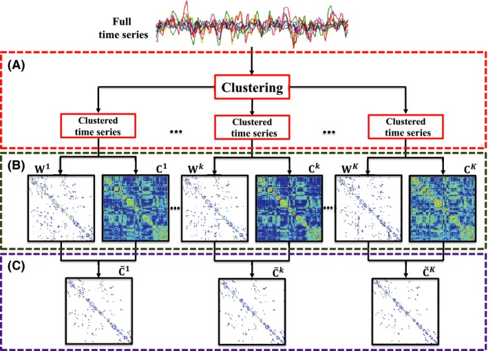
Method Overview. (A) Temporal decomposition of R‐fMRI time series into several clusters based on spatial coherence using k‐means clustering, (B) computation of PC and sparse network matrices for each cluster, and (C) weighting the PC matrix with the corresponding sparse matrix. C is the PC matrix, W is the backbone sparse matrix, and $\tilde{\mathit{C}}$ is the weighted sparse correlation matrix.

1. Cluster, concurrently for all subjects, the time series into multiple clusters with similar spatial activation patterns.

2. For each subject and for each time‐series cluster, construct a PC network that is weighted by the corresponding sparse network.

3. For each subject, concatenate the network matrices from all clusters.

Temporal Decomposition of Functional Time Series

For analysis of short‐time interactive between brain regions, we cluster the time series into subseries that exhibit similar spatial patterns (Figure 2). Let ${\{{\tilde{\mathit{x}}}_d\in {\mathbf{R}}^M\}}_{d=1,\dots ,D^{\prime }}$ be the set of R‐fMRI time series for a subject (D′ = number of time points, and M = number of ROIs). We first concatenate the time series from all N subjects into a matrix $\tilde{\mathit{X}}=[{\tilde{\mathit{x}}}^1,\dots ,{\tilde{\mathit{x}}}^M]\in {\mathbf{R}}^{D\times M}$ where D = N × D′ and ${\tilde{\mathit{x}}}_d$ denotes its d‐th row vector. We then use a k‐means clustering algorithm to partition ${\{{\tilde{\mathit{x}}}_d\}}_{d=1,\dots ,D}$ into K clusters, each with index set J _k, by minimizing the within‐cluster sum of squared errors

$$\text{arg min}{\sum }_{k=1}^k{\sum }_{d\in J_k}{\Vert {\tilde{\mathit{x}}}_d-{\mathit{\mu }}_k\Vert }_2^2,$$ (1)

Figure 2.

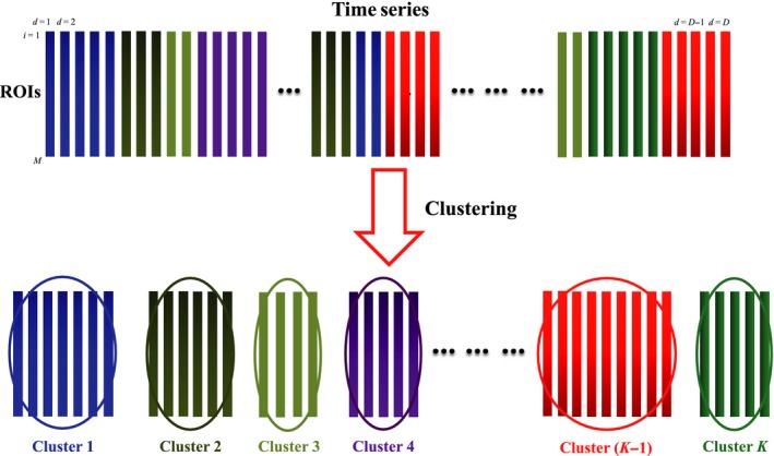
Temporal Decomposition. Temporal decomposition of R‐fMRI time series into subseries with similar patterns of spatial coherence. The colors indicate clusters with similar patterns of spatial activation.

where μ _k denotes the center of k‐th cluster.

Connection Strengths Based on Pearson Correlation and Regression Analysis

After temporal decomposition, the time series from each ROI can be seen as composed of a number of subseries from a number of clusters. For each cluster, we have the data for N subjects, parcellated into M ROIs {x ⁱ}_i=1,…,M, where ${\mathit{x}}^i\in {\mathbf{R}}^{D_k}$ with D _k as the length of the subseries within the k‐th cluster. Note that D _k can vary with subjects and clusters. Thus, the symmetric connectivity matrix C = {C _ij}_j=1,…,M ∈ R ^M × M based on Pearson correlation is computed as

$$C_{ij}=\frac{\text{cov}(x^i,x^j)}{{\mathit{\sigma }}_i{\mathit{\sigma }}_j},$$ (2)

where cov(.,.) is the regional covariance, and σ _i and σ _ij are the standard deviations of x ⁱ and x ^j, respectively.

Brain networks are inherently sparse because neurologically a brain region predominantly interacts with only a small number of other regions. However, the PC networks computed using Eq. (2) typically have dense connections, making them difficult to interpret especially in the presence of spurious connections. Several studies 43, 44, 49, 50 have suggested that certain constraints can be imposed on the networks to identify true connections from noisy connections. The regional mean time‐subseries of the i‐th ROI, out of M ROIs, y ⁱ, can be regarded as a targeted response vector, and the time‐subseries of all other ROIs as predictors:

$${\mathit{y}}^i={\mathit{X}}^i{\mathit{w}}^i+{\mathit{ϵ}}^i,$$ (3)

where ${\mathit{ϵ}}^i$ is the error vector, ${\mathit{y}}^i={\mathit{X}}^i\in {\mathrm{R}}^{D_k}$, ${\mathit{X}}^i=[{\mathit{x}}^{\mathit{1}},\dots ,{\mathit{x}}^{i-\mathit{1}},\mathbf{0},{\mathit{x}}^{i+\mathit{1}},\dots ,{\mathit{x}}^M]\in {\mathbf{\text{R}}}^{D_k\times M}$ is the data matrix with the i‐th column set to zero, and w ⁱ = [w ₁,…,w _i‐1,0,w _i+1,…,w _M]^T∈ R ^M is the weight coefficient vector that quantifies how related the other ROIs are to the i‐th ROI.

Construction of Backbone Sparse Network

To obtain a common backbone network topology across subjects, we impose group sparsity in estimating the connection architecture 44, 51. This is accomplished for the i‐th ROI by solving for each cluster a least‐squares problem that is penalized by l _2,1‐norm:

$${\text{min}}_{{\mathit{w}}^i(1),\dots ,{\mathit{w}}^i(\mathrm{N})}{\sum }_{n=1}^N\Vert {\mathit{y}}^i(\mathrm{n})-{\mathbf{X}}^{\mathrm{i}}(\mathrm{n}){\mathbf{w}}^{\mathrm{i}}{(\mathrm{n})\Vert }_{\mathrm{F}}^2+\mathit{\lambda }{\Vert {\mathbf{w}}^{\mathrm{i}}(1),\dots ,{\mathbf{w}}^{\mathrm{i}}(\mathrm{N})\Vert }_{2,1},$$ (4)

where n = 1,…,N is the subject index, and λ > 0 is the sparsity tuning parameter.

This sparse regression model is applied to each ROI separately to produce a sparse coefficient matrix W(n) = [w ¹(n),…,w ^M(n)]^T ∈R ^M×M. The locations of nonzero elements of W are identical for all subjects, hence giving a backbone network topology. The nonzero elements (i.e., w _ij ≠ 0) indicate that the i‐th and the j‐th ROIs are functionally connected, whereas the zero elements indicate the absence of connections between ROIs. While sharing a common network topology, subject‐specific information is encoded by the actual values of the nonzero elements in W 44. As W is not necessarily symmetric, we symmetrize the backbone network as done in our previous work 44.

Sparse Weighted Functional Connectivity Networks

For each subject and each cluster, a PC network matrix C and a sparse network matrix W are computed. Matrix W discards spurious connections and retains prominent connections. For each ROI, each nonzero value in the associated row of W is an indicator of how well the time series in the ROI can be explained by the time series in each of the other ROIs. Unlike the PC network, connections in the sparse network are computed by considering all ROIs concurrently. We use W to weight C so that the degree of coherence of the functional time series as measured by PC can be modulated by the strength of the connections as given by the sparse network:

$$\tilde{C}=\mathit{W}\circ \mathit{C},$$ (5)

where ○ denotes the Hadamard (or element‐wise) product operator. Grouping the weighted network matrices for all clusters, we have for each subject a family of connectivity matrices ${\{\tilde{\mathit{C}}(k)\}}_{k=1,\dots ,K},$ which can reflect dynamic network change with greater granularity.

Feature Selection and Classifier Learning

We employ the support vector machine (SVM) implemented using the LIBSVM package 52 as our classifier. The optimal SVM models are learned via a nested cross‐validation scheme. Specifically, we randomly partition the subjects in the ASD and TD groups into 10 sets with approximately equal size without overlap. One set is first left out as testing set, and the rest are used as the training set to learn a SVM model. Using the training set, sparse weighted functional connectivity networks are constructed. We then compute, for each ROI, the local clustering coefficient 53, a measure of node cliquishness, from the weighted connectivity matrices as a network summary statistic. As AAL atlas with M = 116 ROIs was utilized to parcellate the brain, a feature vector consisting of 116 clustering coefficients, one for each ROI, can be generated from each network matrix. For each subject, the feature vectors from all clusters are concatenated to generate a long feature vector with K × M elements. We then utilize Lasso 42 to select a small subset of features that are discriminative for ASD diagnosis. The optimal tuning parameters for Lasso and SVM are selected via grid search based on the training set. Parameter combination that gives the best performance is used to construct the optimal SVM model for performance evaluation using the left out testing set. This procedure is repeated ten times, once for each of the 10 training sets to compute the overall cross‐validation classification performance.

Results

Diagnostic Performance

We compared the performance of the proposed method, short‐time sparse regression with Pearson correlation weighting (ST‐SR‐PC), with the methods based on single‐ and multi‐network methods. The single‐network methods are based on the entire time series with connections computed based on (1) Pearson correlation (PC), (2) Sparse regression (SR) 44 and (3) Sparse regression with Pearson correlation weighting (SR‐PC). The multinetwork methods are based on short‐time clusters and (1) short‐time PC (ST‐PC) and (2) short‐time sparse regression (ST‐SR). For the multiple network‐based approach, we evaluated the performance over K = 2,…,7. A linear kernel SVM with trade‐off parameters C = [−5.00, −4.25,…, 10.00] was used in the comparison. The feature selection step was performed by setting the tuning parameter of Lasso λ = [0.05, 0.10,…,0.5]. The combination of parameters, that is, K, C, and λ, that achieved the best classification accuracy based on the training sets was applied to the testing set to compute the final cross‐validation classification performance. We evaluated the diagnostic power of the competing methods using several statistical metrics, that is, the predictive ACCuracy (ACC), SENsitivity (SEN), SPEcificity (SPE), Positive Predictive Value (PPV), and Negative Predictive Value (NPV).

Figure 3 summarizes ASD diagnostic performances of the compared methods obtained based on SVM with linear kernel. The proposed method (ST‐SR‐PC) consistently performs better than the competing methods for most of the evaluation metrics. Specifically, the proposed method always achieved the highest ACC, SEN, and PPV values, indicating its superiority over the single‐network and multinetwork approaches.

Figure 3.

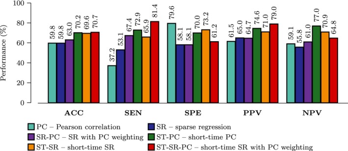
Performance Evaluation. Performance comparison for single‐ and multinetwork approaches using data from NYU. (ACC = ACCuracy, SEN = SENsitivity, SPE = SPEcificity, PPV = Positive Predictive Value, NPV = Negative Predictive Value).

To evaluate the reproducibility and reliability of our proposed framework, we repeated the experiments using data of 4 other centers (namely Stanford, UCLA‐1, UM‐1, and Yale) from ABIDE that contain a reasonably large number of subjects with ages ranging from 7 to 15 years old. The ASD diagnostic performance of the compared methods obtained based on linear SVM was illustrated in Figure 4. Our proposed framework consistently achieved higher diagnostic accuracy than the competing methods for the data from all 4 centers, indicating reproducibility of our framework to other similar datasets.

Figure 4.

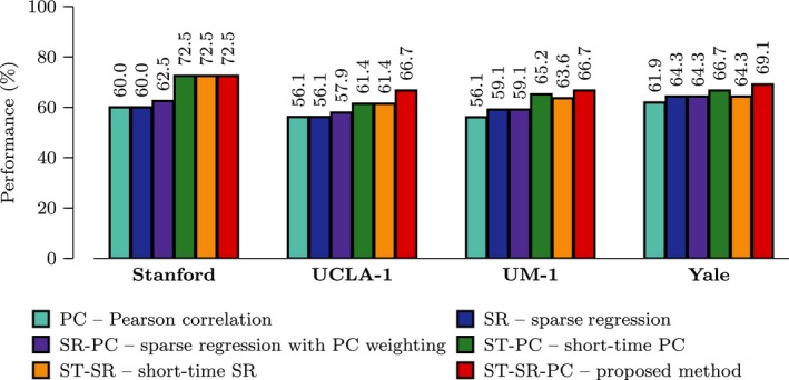
Multi‐site Performance. Performance comparison for single‐ and multinetwork approaches using data from multiple centers.

Effects of SVM Kernel Types

We evaluated the performance of the proposed method when different SVM kernels (linear, radial basis function (RBF), and polynomial) are used. The range for the width parameter of the RBF kernel is γ = [10⁻¹⁶, 10⁻¹⁴,…,10⁻⁶]. The range for the degree parameter of the polynomial kernel is β = [2,…,8]. Two different sets of tradeoff parameters were used for the RBF and polynomial kernels: (1) default trade‐off parameter, C = 1, and (2) optimal parameter determined via grid search using C = [−5.00, −4.25,…, 10.00]. The latter was used for the linear kernel. The results are summarized in Figure 5. For varied C, the linear and RBF kernels performed similarly whereas the polynomial kernel performed slightly worse. For the default C, the linear kernel gives relatively stable results compared with the RBF and polynomial kernels.

Figure 5.

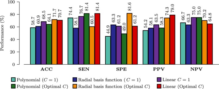
Effects of SVM Kernels. Performance evaluation using different SVM kernels (ACC = ACCuracy, SEN = SENsitivity, SPE = SPEcificity, PPV = Positive Predictive Value, NPV = Negative Predictive Value).

The Most Discriminative Regions

We define the most discriminative regions as the regions that were selected with the highest frequencies during the ten‐fold cross‐validation. Specifically, we first computed the frequency of a feature been selected and used for constructing SVM classifier during training process. We then computed the selection frequency of a region as the summation of selection frequencies of all features that correspond to the same region. Brain regions with the highest final selection frequencies were regarded as the most discriminative regions in this study. Figure 6 graphically shows the top selected regions, which are located on both brain hemispheres and all four lobes, indicating the spread of functional connectivity disruptions throughout the autistic brain. These regions include the subcortical and limbic structures (amygdala, putamen, middle cingulate gyrus, and parahippocampal), frontal (precentral gyrus, middle, superior, and inferior frontal gyri), parietal (superior parietal gyrus, inferior parietal lobule, and precuneus), occipital (cenues, lingual gyrus, and superior occipital gyrus), and temporal (superior and middle temporal poles, and middle temporal gyrus) lobes.

Figure 6.

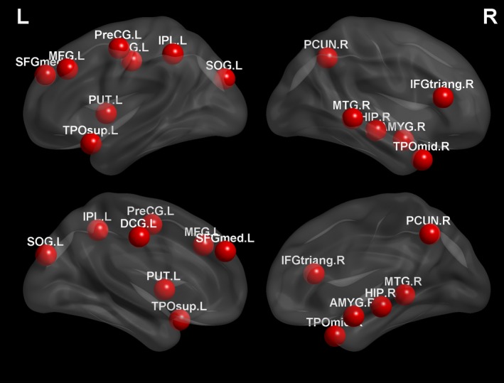
Most discriminative regions. Regions that were selected with the highest frequencies.

Discussion

The human brain is constantly active, even at rest, and neural interactions consistently occur at shorter timescales than an R‐fMRI scanning session of 6–12 min 39, 54, 55, 56, 57. In conventional stationary temporal correlation analysis, one connectivity network is computed per R‐fMRI scan, ignoring dynamic and recurring brain activation patterns. In this work, we suggest to construct multiple functional connectivity networks based on short‐time functional time‐subseries. We cluster the functional time series based on spatial activation patterns into different subseries. A connectivity network is then computed for each cluster to characterize the dynamically varying co‐activation and co‐deactivation patterns among brain regions, allowing a more fine‐grained analysis of brain functional dynamics. On the other hand, fully connected connectivity networks with many spurious connections unable to provide robust and accurate characterization of brain states due to large amount of noise. We thus suggest to construct a more meaningful functional network by weighting the PC with a backbone sparse network derived using all subjects. By considering both temporal coherence and network sparsity, the proposed method ST‐SR‐PC outperforms the second best method, SR‐PC, by 7% in ACC, 14% in SEN, 14% in PPV, and 3% in NPV. Although the classification accuracy of 71% by the proposed method is not high, our result was achieved via a more reliable 10‐fold nested cross‐validation approach, compared to 23, which used the more optimistic leave‐one‐out approach. A recent study 6, which used the similar NYU dataset, achieved an accuracy of 65% when using thresholded networks and a leave‐one‐out cross‐validation. It is also reported that there is no significant difference in terms of classification accuracy between using the full time series and motion scrubbed time series (>50% volumes remained) for this dataset 6.

To evaluate the reproducibility and generalizability of our proposed framework, we have performed ASD diagnosis using the same settings on the data of 4 other centers (namely Stanford, UCLA‐1, UM‐1, and Yale) from ABIDE. Our proposed framework consistently outperformed the competing methods, based on either single network or multiple networks, in all 4 centers. Large heterogeneities in scanning protocols, imaging sequences, acquisition parameters, and subject populations will definitely limit the sensitivity for detecting abnormalities induced by ASD and thus the diagnosis accuracy. The relatively good and consistent performances achieved by the proposed framework on multicenter data, although different classifiers were constructed for different centers, suggest that the multiple network‐based dynamic connectivity approach is relatively robust in identifying subtle disease‐induced neuro‐functional wiring disruptions and can potentially be an effective biomarker for brain disease diagnosis.

In our framework, SVM with linear kernel performs the best, followed by RBF kernel and polynomial kernel. Linear kernel gives the best stability with respect to variation of tradeoff parameter C. With the linear kernel, the classification accuracy varies from 68% to 71%. The nonlinear kernels, on the other hand, experience significant performance drop, that is, more than 5% for the polynomial kernel and more than 10% for the RBF kernel. It has been shown that the linear kernel is more effective than the RBF kernel when the number of features is significantly greater than the number of subjects 58, as in our case. When using the optimal C determined via grid search, our method outperforms all competing methods for all kernels.

Encephalic regions that are associated with ASD pathology have already been extensively reported in previous studies, either based on group‐level comparison 59, 60, 61, 62 or individual‐level discriminative analysis 3, 6, 9, 13, 16, 63, 64. Most of the regions selected by our method have been reported in previous studies to be highly associated with ASD pathologies, particularly the subcortical and limbic structures, which serve as hubs for most connection pathways. It is interesting to observe that several components in the limbic system have been selected in the proposed framework as important features for ASD classification. This may suggest that our framework is able to extract and reflect the relationships between behavioral impairments and functional abnormalities occur in ASD.

The limitations of this work are discussed as follows:

1. We used l _2,1‐norm regularization (group Lasso) to estimate the group‐level backbone sparse connectivity matrix. If highly similar connections exist, the l _2,1‐norm solution will be unstable and will tend to retain only one of these connections and discard the others 65. To overcome this limitation, the elastic net, which adds a ridge regression (‖w‖²) term to the original Lasso, can be used to stabilize the solution. Our future work may include the development and application of ‘group elastic net’ for this purpose.

2. In our current work, the number of clusters, K, needs to be predetermined. To avoid this, a data‐driven approach, for example, affinity propagation algorithm 66, can be used to automatically determine the appropriate number of clusters.

3. Recent findings 67 indicate that one obvious source of heterogeneity in ASD is the gender. As in this work the ratio of male‐to‐female subjects is approximately 5 to 1, the results may be disproportionately skewed. Future research should take into account this issue to reduce the effects of heterogeneity for improving classification performance.

Conclusions

We have presented an effective ASD diagnosis framework that harnesses the short‐time spatiotemporal coherence of functional time series and the sparse nature of brain connectivity. By constructing connectivity networks based on short‐time functional time series, we are able to extract network dynamics that are elusive when the time series is treated as an undivided whole. Imposing group sparsity on the estimated networks trims spurious connections that might confound classification. The combination of these strategies results in improved classification performance, as supported by the experimental results.

Conflict of Interest

There are no conflict of interests including any financial, personal, or other relationships with people or organizations for any of the coauthors related to the work described in the article.

References

- 1. Amaral DG, Schumann CM, Nordahl CW. Neuroanatomy of autism. Trends Neurosci 2008;31:137–145. [DOI] [PubMed] [Google Scholar]
- 2. American Psychiatric Association . Diagnostic and statistical manual of mental disorders (DSM‐5). Arlington, VA: American Psychiatric Publishing (APPI), 2013. [Google Scholar]
- 3. Ecker C, Marquand A, Mourao‐Miranda J, et al. Describing the brain in five dimensions ‐ magnetic resonance imaging‐assisted diagnosis of autism spectrum disorder using a multiparameter classification approach. J Neurosci 2010;30:10612–10623. [DOI] [PMC free article] [PubMed] [Google Scholar]
- 4. Developmental Disabilities Monitoring Network Surveillance Year . Principal Investigators; Centers for Disease Control and Prevention (CDC). Prevalence of autism spectrum disorder among children aged 8 years ‐ autism and developmental disabilities monitoring network, 11 sites, United States, 2010. MMWR Surveill Summ 2014;63:1–21. [PubMed] [Google Scholar]
- 5. Dawson G, Jones EJH, Merkle K, et al. Early behavioral intervention is associated with normalized brain activity in young children with autism. J Am Acad Child Adolesc Psychiatry 2012;51:1150–1159. [DOI] [PMC free article] [PubMed] [Google Scholar]
- 6. Nielsen JA, Zielinski BA, Fletcher PT, et al. Multisite functional connectivity MRI classification of autism: ABIDE results. Front Hum Neurosci 2013;7:599. [DOI] [PMC free article] [PubMed] [Google Scholar]
- 7. Gillbeg C. Autism and related behaviors. J Intellect Disabil Res 1993;37:343–372. [DOI] [PubMed] [Google Scholar]
- 8. Lord C, Jones RM. Annual research review: Re‐thinking the classification of autism spectrum disorders. J Child Psychol Psychiatry 2012;53:490–509. [DOI] [PMC free article] [PubMed] [Google Scholar]
- 9. Wee CY, Wang L, Shi F, Yap PT, Shen D. Diagnosis of autism spectrum disorders using regional and interregional morphological features. Hum Brain Mapp 2014;35:3414–3430. [DOI] [PMC free article] [PubMed] [Google Scholar]
- 10. Jin Y, Wee CY, Shi F, Thung KH, Ni D, Yap PT, Shen D. Identification of infants at high‐risk for autism spectrum disorder using multiparameter multiscale white matter connectivity networks. Hum Brain Mapp 2015;36:4880–4896. [DOI] [PMC free article] [PubMed] [Google Scholar]
- 11. Boddaert N, Chabane N, Gervais H, et al. Superior temporal sulcus anatomical abnormalities in childhood autism: A voxel‐based morphometry MRI study. NeuroImage 2004;23:364–369. [DOI] [PubMed] [Google Scholar]
- 12. Brambilla P, Hardan A, di Nemi SU, Perez J, Soares JC, Barale F. Brain anatomy and development in autism: Review of structural MRI studies. Brain Res Bull 2003;61:557–569. [DOI] [PubMed] [Google Scholar]
- 13. Ecker C, Rocha‐Rego V, Johnston P, et al. Investigating the predictive value of whole‐brain structural MR scans in autism: A pattern classification approach. NeuroImage 2010;49:44–56. [DOI] [PubMed] [Google Scholar]
- 14. Lo YC, Soong WT, Gau SSF, et al. The loss of asymmetry and reduced interhemispheric connectivity in adolescents with autism: A study using diffusion spectrum imaging tractography. Psychiatry Res 2011;192:60–66. [DOI] [PubMed] [Google Scholar]
- 15. Allen G, Courchesne E. Differential effects of developmental cerebellar abnormality on cognitive and motor functions in the cerebellum: An fMRI study of autism. Am J Psychiatry 2003;160:262–273. [DOI] [PubMed] [Google Scholar]
- 16. Anderson JS, Druzgal TJ, Froehlich A, et al. Decreased interhemispheric functional connectivity in autism. Cereb Cortex 2011;21:1134–1146. [DOI] [PMC free article] [PubMed] [Google Scholar]
- 17. Delmonte S, Gallagher L, O'Hanlon E, McGrath J, Balsters JH. Functional and structural connectivity of frontostriatal circuitry in autism spectrum disorder. Front Hum Neurosci 2013;7:430. [DOI] [PMC free article] [PubMed] [Google Scholar]
- 18. Bassett DS, Bullmore ET. Small‐world brain networks. Neuroscientist 2006;12:512–523. [DOI] [PubMed] [Google Scholar]
- 19. Bullmore E, Sporns O. Complex brain networks: Graph theoretical analysis of structural and functional systems. Nat Rev Neurosci 2009;10:186–198. [DOI] [PubMed] [Google Scholar]
- 20. He Y, Chen Z, Evans A. Small‐world anatomical networks in the human brain revealed by cortical thickness from MRI. Cereb Cortex 2007;17:2407–2419. [DOI] [PubMed] [Google Scholar]
- 21. He Y, Evans A. Graph theoretical modeling of brain connectivity. Curr Opin Neurol 2010;23:341–350. [DOI] [PubMed] [Google Scholar]
- 22. He Y, Wang J, Wang L, et al. Uncovering intrinsic modular organization of spontaneous brain activity in humans. PLoS ONE 2009;4:1–17. [DOI] [PMC free article] [PubMed] [Google Scholar]
- 23. Anderson JS, Nielsen JA, Froehlich AL, et al. Functional connectivity magnetic resonance imaging classification of autism. Brain 2011;134:3742–3754. [DOI] [PMC free article] [PubMed] [Google Scholar]
- 24. Achard S, Salvador R, Whitcher B, Suckling J, Bullmore ET. A resilient, low‐frequency, small‐world human brain functional network with highly connected association cortical hubs. J Neurosci 2006;26:63–72. [DOI] [PMC free article] [PubMed] [Google Scholar]
- 25. Dosenbach NUF, Fair DA, Miezin FM, et al. Distinct brain networks for adaptive and stable task control in humans. Proc Natl Acad Sci USA 2007;104:11073–11078. [DOI] [PMC free article] [PubMed] [Google Scholar]
- 26. Greicius MD, Srivastava G, Reiss AL, Menon V. Default‐mode network activity distinguishes Alzheimer's disease from healthy aging: Evidence from functional MRI. Proc Natl Acad Sci USA 2004;101:4637–4642. [DOI] [PMC free article] [PubMed] [Google Scholar]
- 27. Rombouts SARB, Barkhof F, Goekoop R, Stam CJ, Scheltens P. Altered resting state networks in mild cognitive impairment and mild Alzheimer's disease: An fMRI study. Hum Brain Mapp 2005;26:231–239. [DOI] [PMC free article] [PubMed] [Google Scholar]
- 28. Supekar K, Menon V, Rubin D, Musen M, Greicius MD. Network analysis of intrinsic functional brain connectivity in Alzheimer's disease. PLoS Comput Biol 2008;4:e1000100. [DOI] [PMC free article] [PubMed] [Google Scholar]
- 29. Tomasi D, Volkow ND. Functional connectivity density mapping. Proc Natl Acad Sci USA 2010;107:9885–9890. [DOI] [PMC free article] [PubMed] [Google Scholar]
- 30. Wang J, Zuo X, He Y. Graph‐based network analysis of resting‐state functional MRI. Front Syst Neurosci 2010;4:16. [DOI] [PMC free article] [PubMed] [Google Scholar]
- 31. Wang J, Zuo X, Gohel S, Milham MP, Biswal BB, He Y. Graph theoretical analysis of functional brain networks: Test‐retest evaluation on short‐ and long‐term resting‐state functional MRI data. PLoS ONE 2011;6:e21976. [DOI] [PMC free article] [PubMed] [Google Scholar]
- 32. Wee CY, Yap PT, Zhang D, et al. Identification of MCI individuals using structural and functional connectivity networks. NeuroImage 2012;59:2045–2056. [DOI] [PMC free article] [PubMed] [Google Scholar]
- 33. Wee CY, Yap PT, Denny K, et al. Resting‐state multi‐spectrum functional connectivity networks for identification of MCI patients. PLoS ONE 2012;7:e37828. [DOI] [PMC free article] [PubMed] [Google Scholar]
- 34. Jie B, Zhang D, Wee CY, Shen D. Topological graph kernel on multiple thresholded functional connectivity networks for mild cognitive impairment classification. Hum Brain Mapp 2014;35:2876–2897. [DOI] [PMC free article] [PubMed] [Google Scholar]
- 35. Jie B, Zhang D, Gao W, Wang Q, Wee CY, Shen D. Integration of network topological and connectivity properties for neuroimaging classification. IEEE Trans Biomed Eng 2014;61:576–589. [DOI] [PMC free article] [PubMed] [Google Scholar]
- 36. Suk HI, Wee CY, Lee SW, Shen D. Supervised discriminative group sparse representation for mild cognitive impairment diagnosis. Neuroinformatics 2014;13:277–295. [DOI] [PMC free article] [PubMed] [Google Scholar]
- 37. Van Dijk KRA, Hedden T, Venkataraman A, Evans KC, Lazar SW, Buckner RL. Intrinsic functional connectivity as a tool for human connectomics: Theory, properties, and optimization. J Neurophysiol 2010;103:297–321. [DOI] [PMC free article] [PubMed] [Google Scholar]
- 38. Liu X, Duyn JH. Time‐varying functional network information extracted from brief instances of spontaneous brain activity. Proc Natl Acad Sci USA 2013;110:4392–4397. [DOI] [PMC free article] [PubMed] [Google Scholar]
- 39. Smith SM, Miller KL, Moeller S, et al. Temporally‐independent functional modes of spontaneous brain activity. Proc Natl Acad Sci USA 2012;109:3131–3136. [DOI] [PMC free article] [PubMed] [Google Scholar]
- 40. Tagliazucchi E, Balenzuela P, Fraiman D, Chialvo DR. Criticality in large‐scale brain fMRI dynamics unveiled by a novel point process analysis. Front Physiol 2012;3:15. [DOI] [PMC free article] [PubMed] [Google Scholar]
- 41. Damaraju E, Allen EA, Belger A, et al. Dynamic functional connectivity analysis reveals transient states of dysconnectivity in schizophrenia. Neuroimage Clin 2014;5:298–308. [DOI] [PMC free article] [PubMed] [Google Scholar]
- 42. Tibshirani R. Regression shrinkage and selection via the LASSO. J Roy Stat Soc 1996;58:267–288. [Google Scholar]
- 43. Varoquaux G, Gramfort A, Poline JB, Thirion B. Brain covariance selection: Better individual functional connectivity models using population prior. Adv Neural Inf Process Syst'10 2010;23:2334–2342. [Google Scholar]
- 44. Wee CY, Yap PT, Zhang D, Wang L, Shen D. Group‐constrained sparse fMRI connectivity modeling for mild cognitive impairment identification. Brain Struct Funct 2014;219:641–656. [DOI] [PMC free article] [PubMed] [Google Scholar]
- 45. Di Martino A, Mostofsky S. Autism Brain Imaging Data Exchange.
- 46. American Psychiatric Association . Diagnostic and statistical manual of mental disorders, fourth edition ‐ text revision (DSMIV‐TR). Arlington, VA: American Psychiatric Association, 2000. [Google Scholar]
- 47. Friston KJ, Williams S, Howard R, Frackowiak RS, Turner R. Movement‐related effects in fMRI time‐series. Magn Reson Med 1996;35:346–355. [DOI] [PubMed] [Google Scholar]
- 48. Tzourio‐Mazoyer N, Landeau B, Papathanassiou D, et al. Automated anatomical labeling of activations in SPM using a macroscopic anatomical parcellation of the MNI MRI single‐subject brain. NeuroImage 2002;15:273–289. [DOI] [PubMed] [Google Scholar]
- 49. Huang S, Li J, Sun L, et al. Learning brain connectivity of Alzheimer's disease by sparse inverse covariance estimation. NeuroImage 2010;50:935–949. [DOI] [PMC free article] [PubMed] [Google Scholar]
- 50. Lee H, Lee DS, Kang H, Kim BN, Chung MK. Sparse brain network recovery under compressed sensing. IEEE Trans Med Imaging 2011;30:1154–1165. [DOI] [PubMed] [Google Scholar]
- 51. Zhang D, Shen D; Alzheimer's Disease Neuroimaging Initiative . Predicting future clinical changes of MCI patients using longitudinal and multimodal biomarkers. PLoS ONE 2012;7:e33182. [DOI] [PMC free article] [PubMed] [Google Scholar]
- 52. Chang CC, Lin CJ. LIBSVM: A library for support vector machines. ACM Trans Intell Syst Technol 2011;2:27:1‐. [Google Scholar]
- 53. Rubinov M, Sporns O. Complex networks measures of brain connectivity: Uses and interpretations. NeuroImage 2010;52:1059–1069. [DOI] [PubMed] [Google Scholar]
- 54. Allen EA, Damaraju E, Plis SM, Erhardt EB, Eichele T, Calhoun VD. Tracking whole‐brain connectivity dynamics in the resting state. Cereb Cortex 2014;24:663–676. [DOI] [PMC free article] [PubMed] [Google Scholar]
- 55. Chang C, Glover GH. Time‐frequency dynamics of resting‐state brain connectivity measured with fMRI. NeuroImage 2010;50:81–98. [DOI] [PMC free article] [PubMed] [Google Scholar]
- 56. Handwerker DA, Roopchansingh V, Gonzalez‐Castillo J, Bandettini PA. Periodic changes in fMRI connectivity. NeuroImage 2012;63:1712–1719. [DOI] [PMC free article] [PubMed] [Google Scholar]
- 57. Hutchison RM, Womelsdorf T, Allen EA, et al. Dynamic functional connectivity: Promises, issues, and interpretations. NeuroImage 2013;80:360–368. [DOI] [PMC free article] [PubMed] [Google Scholar]
- 58. Song S, Zhan Z, Long Z, Zhang J, Yao L. Comparative study of SVM methods combined with voxel selection for object category classification on fMRI data. PLoS ONE 2011;6:e17191. [DOI] [PMC free article] [PubMed] [Google Scholar]
- 59. Hardan AY, Muddasani S, Vemulapalli M, Keshavan MS, Minshew NJ. An MRI study of increased cortical thickness in autism. Am J Psychiatry 2006;163:1290–1292. [DOI] [PMC free article] [PubMed] [Google Scholar]
- 60. McAlonan GM, Cheung V, Cheung C, et al. Mapping the brain in autism. A voxel‐based MRI study of volumetric differences and intercorrelations in autism. Brain 2005;128:268–276. [DOI] [PubMed] [Google Scholar]
- 61. Nordahl CW, Dierker D, Mostafavi I, et al. Cortical folding abnormalities in autism revealed by surface‐based morphometry. J Neurosci 2007;27:11725–11735. [DOI] [PMC free article] [PubMed] [Google Scholar]
- 62. Redcay E, Courchesne E. Deviant functional magnetic resonance imaging patterns of brain activity to speech in 2‐3‐year‐old children with autism spectrum disorder. Biol Psychiatry 2008;64:589–598. [DOI] [PMC free article] [PubMed] [Google Scholar]
- 63. Uddin LQ, Menon V, Young CB, et al. Multivariate searchlight classification of structural magnetic resonance imaging in children and adolescents with autism. Biol Psychiatry 2011;70:833–841. [DOI] [PMC free article] [PubMed] [Google Scholar]
- 64. Wang H, Chen C, Fushing H. Extracting multiscale pattern information of fMRI based functional brain connectivity with application on classification of autism spectrum disorders. PLoS ONE 2012;7:e45502. [DOI] [PMC free article] [PubMed] [Google Scholar]
- 65. Zou H, Hastie T. Regularization and variable selection via the elastic net. J R Statist Soc B 2005;67:301–320. [Google Scholar]
- 66. Frey BJ, Dueck D. Clustering by passing messages between data points. Science 2007;315:972–976. [DOI] [PubMed] [Google Scholar]
- 67. Lai MC, Lombardo MV, Suckling J, et al. Biological sex affects the neurobiology of autism. Brain 2013;136:2799–2815. [DOI] [PMC free article] [PubMed] [Google Scholar]